inverse spectral problem for the Schrödinger operator on the square lattice
11footnotetext: Department of Applied Mathematics, School of Mathematics and Statistics, Nanjing University of Science and Technology, Nanjing, 210094, Jiangsu, China, Email: [email protected]22footnotetext: Department of Applied Mathematics, School of Mathematics and Statistics, Nanjing University of Science and Technology, Nanjing, 210094, Jiangsu, China, Email: [email protected]33footnotetext: S.M. Nikolskii Mathematical Institute, Peoples’ Friendship University of Russia (RUDN University), 6 Miklukho-Maklaya Street, Moscow, 117198, Russian Federation, Email: [email protected]Abstract: We consider an inverse spectral problem on a quantum graph associated with the square lattice. Assuming that the potentials on the edges are compactly supported and symmetric, we show that the Dirichlet-to-Neumann map for a boundary value problem on a finite part of the graph uniquely determines the potentials. We obtain a reconstruction procedure, which is based on the reduction of the differential Schrödinger operator to a discrete one. As a corollary of the main results, it is proved that the S-matrix for all energies in any given open set in the continuous spectrum uniquely specifies the potentials on the square lattice.
Keywords: inverse spectral problem, Schrödinger operator, square lattice, Dirichlet-to-Neumann map, inverse scattering
1. introduction
Recently, there have been a lot of studies on quantum graphs, which are one-dimensional Schrödinger (Sturm-Liouville) operators acting on the edges of a metric graph, while some matching conditions are imposed at the graph vertices. Such operators are used for modeling various processes on graph-like structures in physics, mechanics, chemistry, and other applications. Expositions of spectral theory results for quantum graphs can be found, e.g., in the monographs [13, 8, 9, 12] and references therein.
This paper is mostly focused on inverse spectral and scattering problems. Such problems consist in the reconstruction of unknown operator characteristics from spectral information. Till now, inverse problems have been studied for several types of quantum graphs. Reconstruction of differential operators on compact graphs has been investigated in [6, 7, 10, 16, 23, 24, 28, 29, 30] and other studies. Inverse spectral-scattering problems on non-compact graphs with finite and infinite edges were solved, e.g., in [11, 17, 27].
In recent years, Schrödinger operators on infinite periodic graphs have attracted considerable attention of scholars in connection with applications in material studies and nanotechnology (see [22, 20] and references therein). Spectral properties of such operators were studied in [22, 20, 21, 25, 26] and other papers. We also mention that in [14] some spectral theory issues were considered for infinite quantum graphs of general structure (not necessarily periodic). However, to the best of the authors’ knowledge, there were no studies on inverse problems for differential Schrödinger operators on periodic graphs except for the two preprints [4, 5] of Ando et al. Let us discuss their results in more detail.
The two preprints [4, 5] present the same results on the inverse scattering for the Schrödinger operator on the hexagonal lattice with finitely supported potential. The authors of [4, 5] have shown that, in this case, the scattering matrix (S-matrix) uniquely determines the Dirichlet-to-Neumann (D-N) map for a boundary value problem on a finite part of the graph. Furthermore, the differential (continuous) operator was reduced to a difference (discrete) one and the potentials on the graph edges were reconstructed from the D-N map. Thus, it has been shown that the S-matrix uniquely specifies a finitely supported potential on the hexagonal lattice. The preprints [4, 5] continue the previous studies of their authors [1, 2, 3, 18, 19], in which analogous ideas and methods were developed for the inverse scattering on discrete periodic graphs. The difference between [4] and [5] is that, in [5], the preliminary steps up to determining the D-N map by the S-matrix are implemented for the hexagonal lattice, while in [4] they are provided for a general periodic lattice. This opens a perspective of studying inverse spectral problems for different types of periodic graphs.
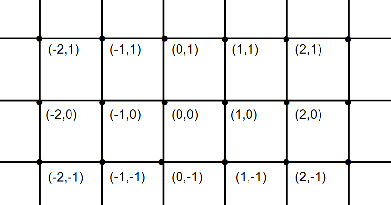
This paper is concerned with a family of one-dimensional Schrödinger operators defined on the edges of the square lattice as in Figure 1, assuming the Kirchhoff conditions at the vertices (the details are given in Section 2). Here, varies over the interval and , where is the set of all edges of the square lattice.
Let us impose the following assumptions on the potentials.
(Q-1) is real-valued, and .
(Q-2) on except for a finite number of edges.
(Q-3) for .
Since the support of the potential is finite, we can choose a sufficiently large square domain such that is located inside of and consider the edge Dirichlet-to-Neumann map associated with this domain (see Section 2 for details). This paper is devoted to the following inverse spectral problem.
Inverse Problem 1.1.
Given the edge D-N map , find the potential .
The main results of this paper are the uniqueness theorem (Theorem 2.1) for Inverse Problem 1.1 and the reconstruction procedure in Section 5. For solving Inverse Problem 1.1, we use the relation between the edge D-N map and the vertex D-N map, which is defined in Section 3. In other words, we reduce the continuous problem to the discrete one. Consequently, we develop a constructive algorithm for the recovery of the potentials from the vertex D-N map. Note that, although we follow the general idea of Ando et al, our reconstruction procedure is different from [4, 5]. First, our algorithm is based on specific properties of the square lattice. Second, the authors of [4, 5] apply the strategy of recovering the potentials along any zigzag line, which perfectly works for discrete operators with constant coefficients [3, 19] but causes difficulties for the reduced vertex Laplacian whose coefficients depend on the unknown potentials (see Remark 5.1 for details). In this paper, we step-by-step recover together with the Laplacian coefficients required at the next steps. For reconstruction of the potential on each fixed edge, we use the classical results of the inverse spectral theory for the Schrödinger operators on finite intervals (see, e.g., [15]). Finally, our results imply the uniqueness for solution of the inverse scattering problem by the S-matrix on the square lattice.
It is worth mentioning that Inverse Problem 1.1 can be treated as the inverse spectral problem on a finite metric graph by the Weyl matrix associated to the boundary vertices. However, our results are novel in this direction. It is well-known the the Weyl matrix uniquely specifies the Schrödinger operator on a tree-graph (see [7, 28]). But, for graphs with cycles, this is not the case in general. Even for the simplest graphs with loops additional data are required (see [24, 30]). Our paper provides a new class of finite quantum graphs whose potentials are uniquely determined by the Weyl matrix. Here, the symmetry of the potentials (Q-3) is crucial.
The paper is organized as follows. In Section 2, we give the definitions related to the edge Schrödinger operator and the edge D-N map. In Section 3, we define the reduced vertex Laplacian and the vertex D-N map, and study the relation between the edge D-N map and the vertex D-N map. In Section 4, some auxiliary solutions of the vertex Schrödinger equation are obtained. In Section 5, we reconstruct the potentials from the D-N map. In Section 6, the inverse scattering by the S-matrix is discussed.
2. Edge Laplacian and Dirichlet-to-Neumann map
Let us define an infinite square lattice with the vertex set
and the edge set
In other words, we consider the vertices as points on the complex plane and suppose that two vertices are joined by an edge if the distance between them equals . For two vertices , the notation means that there exists an edge such that are end points of .
Let each edge be endowed with arclength metric and identified with the interval , where . Put
Let . Then, we call a function on if each () is a function on . We will write that if for all , where is any functional class, e.g., , etc. For , , and , introduce the notations
In other words, is the value of the function and , of its derivative in the vertex along the edge .
Let be a vertex such that . Then, we say that satisfies the Kirchhoff conditions at if
(K-1) is continuous at , that is, for any . In this case, we denote , .
(K-2) and .
We will also use the notation if is the only edge in incident to the vertex , that is, .
Let us define the Schrödinger operator on a finite subgraph of the square lattice. Suppose that the potential satisfies the assumptions (Q-1), (Q-2), and (Q-3). Let be the vertex set of some connected finite subgraph of the lattice . Denote
| (1) | |||
Thus, is the edge set of the subgraph with the vertices . The notations , , , and are used for the interior vertices, the boundary vertices, the interior edges, and the boundary edges, respectively, of the subgraph .
Denote by and call the edge Laplacian the second derivative operation along each edge:
For the subgraph , consider the Dirichlet boundary value problem for the edge Laplacian
| (2) |
where a function is assumed to fulfill the Kirchhoff conditions at every interior vertex and is a function given on the set of the boundary vertices.
Denote by the operator acting by the rule , whose domain is the set of all the functions satisfying the Dirichlet condition at any boundary vertex and the Kirchhoff conditions at any interior vertex . By the standard argument, the operator is self-adjoint and its spectrum is a countable set of real eigenvalues. Below, we assume that
| (3) |
The edge Dirichlet-to-Neumann (D-N) map is defined as follows:
| (4) |
where is the solution of the boundary value problem (2) for the boundary data and is the edge of having as its end point. Below we assume that the vertex set is fixed and use the short notation . Note that can be treated as a vector of , , and , as the matrix function such that , . The matrix function is analytic in satisfying (3).
For simplicity, we consider the domain
where a natural number is chosen so large that . In other words, on all the edges except . In Section 6, we show that the D-N map is uniquely specified by the S-matrix and vice versa, so the form of the domain is actually unimportant.
Consider Inverse Problem 1.1 for the domain . In fact, we have to find the potential on , since on all the other edges . Our main result is the following uniqueness theorem.
Theorem 2.1.
Suppose that the potential on the square lattice satisfies (Q-1), (Q-2), and (Q-3) and is the edge Dirichlet-to-Neumann map for the region such that and . Then uniquely specifies the potential .
3. Reduced vertex Laplacian
The proof of Theorem 2.1 is based on the reduction of the edge Laplacian to the vertex one.
Consider the Schrödinger equation
| (5) |
on each fixed edge . Let be the solutions of (5) with the initial data and , respectively.
Denote by the Schrödinger operator with the domain which consists of functions satisfying the Dirichlet conditions . It is well-known that the operator is self-adjoint and its spectrum is a countable set of real eigenvalues. In the following, we assume that , . This guarantees that and .
If are two end points of an edge , then we denote
Note that, by the assumption (Q-3), we have , hence . In particular, if , then .
We define the reduced vertex Laplacian on by
| (6) |
for . We also define the scalar multiplication operator:
| (7) |
Lemma 3.1.
Let be a fixed vertex. If a function satisfies equation (5) for all and the Kirchhoff conditions in , then the relation holds at .
Proof.
Consider the solutions and of equation of (5) satisfying the initial conditions and . Then, any solution of (5) can be written as
| (8) |
where and are constants.
Let be fixed. For convenience, suppose that for all . Then (8) together with (K-1) imply (see Figure 2):
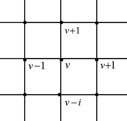
and (K-2) implies
By (8), we have
Thus,
| (9) |
Note that and, under the assumption (Q-3), . Consequently, we arrive at the relation . ∎
Consider the vertex set defined by (1) for and the interior boundary value problem
| (10) |
By virtue of Lemma 3.1, if a function solves the edge boundary value problem (2), then its values in the vertices satisfy (10).
Define the vertex degree in the subgraph as follows:
Then, the vertex D-N map is defined by
Below we use a shorter notation . Note that, for the region , the degrees of the boundary vertices equal to . Hence
| (11) |
The edge and the vertex D-N maps are closely related to each other, which is shown in the following lemma.
Lemma 3.2.
Proof.
Therefore, Inverse Problem 1.1 of recovering the potential from the edge D-N map can be easily reduced to the following inverse problem.
Inverse Problem 3.1.
Given the vertex D-N map , find the potential .
4. Special solutions of the vertex Schrödinger equation
We are now in a position to construct the solution of Inverse Problem 3.1. For this purpose, we first obtain some special solutions of the vertex Schrödinger equation
The boundary of the domain consists of the four parts, see Figure 3:
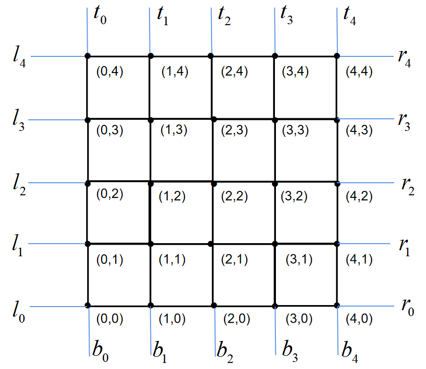
Recall that is the vertex D-N map defined by (11). The key to the inverse procedure is the following partial data problem.
Lemma 4.1.
(1) Given a partial Dirichlet data on , and a partial Neumann data on , there is a unique solution in of the boundary value problem
| (23) |
where
(2) Given the D-N map , a partial Dirichlet data on and a partial Neumann data on , there exists a unique on such that on and on .
Proof.
(1) The values of are computed from the values of . Using equation (23), the Dirichlet data and the known values of , one can then compute . Next, we obtain the values of . Repeating this procedure, we get for all .
(2) For subsets , we denote the associated submatrix of by . Suppose on and on . By (1) and the boundary conditions, the solution vanishes in identically. Hence on . This implies the submatrix
is a bijection. We seek in the form
where
This proves the lemma. ∎
Now, for , let us consider the diagonal line
| (24) |
The vertices on are written as
| (25) |
where .
Lemma 4.2.
Let . Then, there exists a unique solution in of the boundary value problem
| (26) |
with partial Dirichlet data such that
| (27) |
and partial Neumann data on . It satisfies
| (28) |
Proof.
An important feature of the solution in Lemma 4.2 is that vanishes below the line . For such solutions, we obtain the following property.
5. Reconstruction procedure
The goal of this section is to prove Theorem 2.1 on the uniqueness of the inverse spectral problem solution. The proof consists in a reconstruction procedure, which is based on the reduction to the discrete inverse problem by the vertex D-N map (i.e. Inverse Problem 3.1), on specific properties of the square lattice, and on applying the classical results for the recovery of the Schrödinger potential on each edge.
Before proceeding to the reconstruction, we provide two well-known results for inverse spectral problems on a finite interval. Let be a fixed edge. Clearly, the eigenvalues of the Dirichlet problem
coincide with the zeros of the characteristic function .
Lemma 5.1.
([15, Theorem 1.4.3]) If the potential is symmetric, then the Dirichlet eigenvalues for the operator on uniquely determine the potential . In other words, is uniquely specified by the function .
Lemma 5.2.
([15, Theorem 1.4.7]) The Weyl function uniquely specifies the potential .
The both inverse problems of Lemmas 5.1 and 5.2 can be solved constructively by the well-known methods, e.g., the Gelfand-Levitan method and the method of spectral mappings (see [15]).
Now, let us prove Theorem 2.1 by providing a reconstruction procedure for solving Inverse Problem 1.1.
Reconstruction procedure. Suppose that the potential on the square lattice fulfills the conditions (Q-1), (Q-2), and (Q-3). Let be the square region defined in Section 2 and let the corresponding edge D-N map be given.
Step 1. We obtain the vertex D-N map by the formula (12).
Step 2. For , implement the following steps 3–5.
Step 3. For the value of fixed at step 2, draw the line defined by (24) and take the boundary data having the properties in Lemma 4.2. Under the assumption (Q-2), we have on all the boundary edges . So, we know the functions for . By Lemma 4.1 (2), we can find on with the vertex D-N map . Thus, we know on .
Step 4. If , using (11) and the value of , we find
By (30), we have
| (31) |
and
| (32) |
By the known values , , , , , we can find
| (33) |
and
| (34) |
Note that the zeros of and are the Dirichlet eigenvalues for the operator on . Since the potential is symmetric, by Lemma 5.1, these eigenvalues uniquely determine the potentials on and .
Step 5. If , then implement steps 5.1–5.6.
Step 5.1 Using (11) and the values of , , we find
By (30), we get
| (35) |
and
| (36) |
Then, by Lemma 5.1, the zeros of and uniquely determine the potentials on and .
Step 5.2. Evaluating equation (29) at , we obtain
Then, we can get the value of . By (7), we have
where the values of , and are known.
Step 5.3. Obtain the value
| (37) |
which is the Weyl function associated with the potential on .
Step 5.4. Similarly to steps 5.2–5.3, evaluating equation (29) at , we get the Weyl function
| (38) |
associated to the potential on .
Step 5.5. Repeating the procedure analogous to steps 5.2–5.4, we can obtain the values of and .
Step 5.6. The potentials on and are uniquely determined by the Weyl functions by Lemma 5.2.
Thus, we have constructed all the potentials on the upper triangular region of the square domain.
Step 6. Rotate the whole system by the angle and take a square domain congruent to the previous one. Repeat the steps 2–5 to determine the potentials on all the remaining edges of .
This reconstruction procedure determines the potential uniquely on each edge, so it implies the proof of Theorem 2.1.
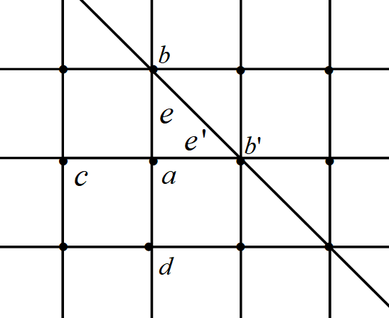
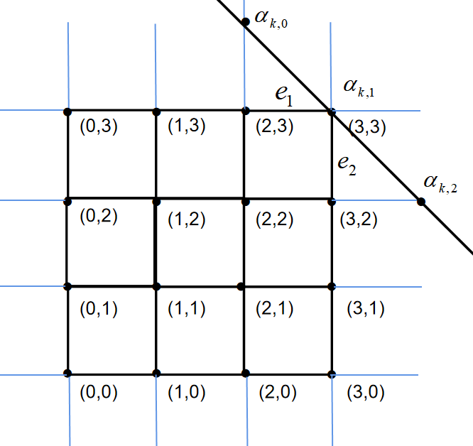
Here we give a simple example of the reconstruction for .
As in Figure 5, by step 4, we get by the D-N map. By (33) and (34), we obtain
Then, the potentials on are determined by Lemma 5.1.
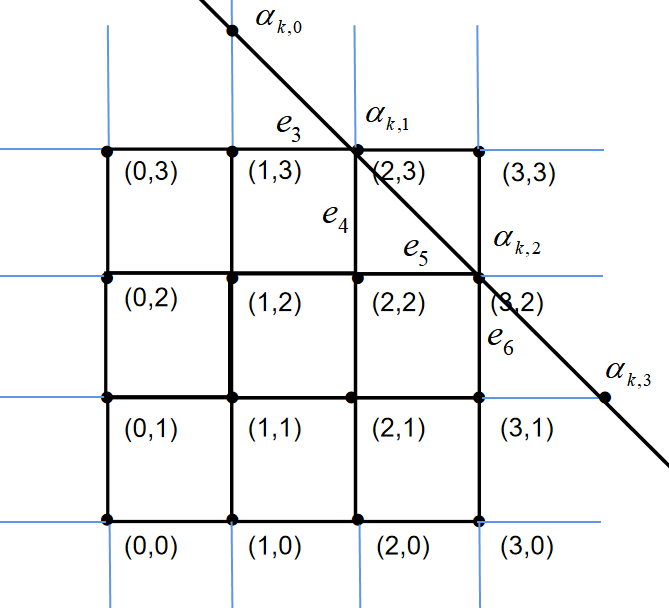
As in Figure 6, by (35),(36), we obtain
Then, the potentials on are determined. By (37) and (38), we have
and
Then, we can determine the potentials on by Lemma 5.2.
As in Figure 7, by (35),(36) in step 5, we get
Then, by using Lemma 5.1, the potentials on are specified.
By (37),(38) and the argument in step 5, we get the values of , , and . Then, the potentials on are determined by Lemma 5.2.
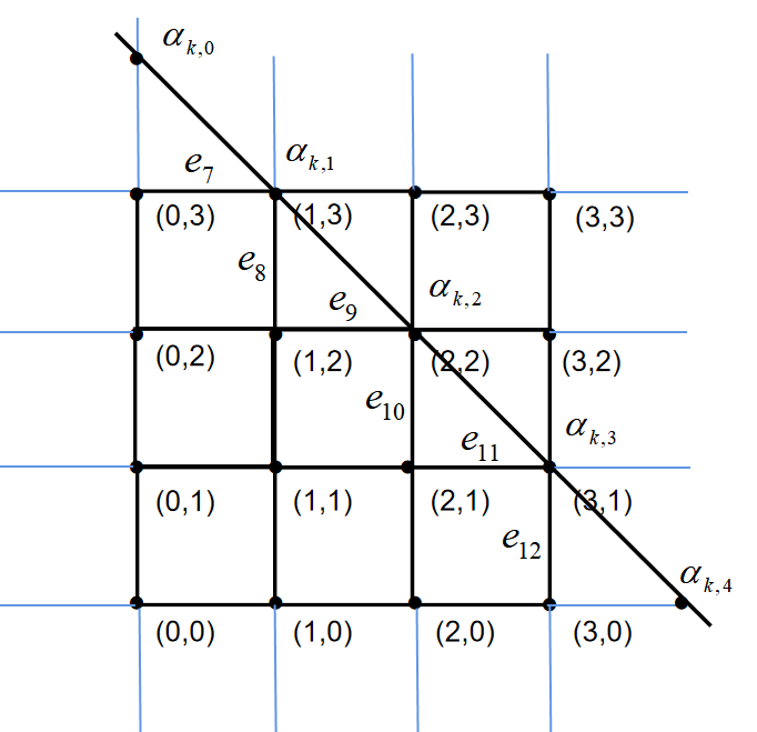
By step 6, rotate the whole system by the angle and the potentials on the rest of edges are determined.
Remark 5.1.
Note that our reconstruction procedure is different from the one provided in [4, 5]. First, our algorithm depends on specific properties of the square lattice, while the procedure in [4, 5] was developed for the hexagonal lattice. Second, the reconstruction strategies differ. The authors of [4, 5] fix an arbitrary line and compute the solution of the boundary value problem generated by the reduced vertex Laplacian according to the analog of Lemma 4.2 for the hexagonal lattice. Then, they consider a zigzag line and find the ratios of the functions for adjacent edges of that line. This helps to recover the potentials . This method perfectly works for the discrete Schrödinger operators with constant coefficients (see [3, 19]). But the analogous treatment of the reduced vertex Laplacian causes difficulties, since the both and depend on some potentials . Therefore, the solution cannot be found until the potentials are known. In our procedure, this problem does not arise, because we step-by-step reconstruct the potentials together with the reduced vertex Laplacian coefficients, which are needed at the next steps. A similar approach can be applied to the hexagonal lattice to improve the algorithm of [4, 5].
6. Inverse scattering problem by the S-matrix
This section is concerned with the inverse scattering problem for the Schrödinger operator by the S-matrix. It has been shown in [4] that the edge D-N map uniquely specifies the S-matrix. Consequently, the uniqueness theorem by the D-N map (Theorem 2.1) implies the uniqueness of solution for the inverse scattering problem. In this section, we provide the definition of the S-matrix , following the papers [2, 4, 5] and show that it uniquely determines the potential on the square lattice.
In this section, it will be convenient for us to associate the vertex set of the square lattice with . In other words, every vertex is a pair of integers . Define the vertex Laplacian
which is self-adjoint on equipped with the inner product
Put and define the discrete Fourier transform by
| (39) |
The adjoint operator is given by
| (40) |
Then, on , is the operator of multiplication by
| (41) |
For , we denote by . By Lemma 3.1 of [2], we define the characteristic surface of by
which is smooth if . We put
| (42) |
where the operator was defined for equation (5) in Section 3.
The resolvent is written as
We put
Their adjoints acting from to are defined for by
Define the operator by
| (43) |
The adjoint operator has the form
For , we denote by . Then,
and
Under the assumptions (Q-1), (Q-2), (Q-3), we define the Schrödinger operator
with domain consisting of functions such that satisfy the Kirchhoff condition (K-1) and (K-2) in all the vertices and . Due to [4], the operator is self-adjoint with the essential spectrum . Furthermore, is absolutely continuous, where is defined by (42). Then, one can introduce the S-matrix for .
Define the spaces and by
where . For , we use the notation in the following sense:
Now, we give the definition of the S-matrix . The following lemma is a special case of Theorem 5.8 from [4].
Lemma 6.1 ([4]).
Let . Then, for any incoming data , there exist a unique solution of the equation
satisfying the Kirchoff conditions, and an outgoing data satisfying
| (44) |
where , is the eigenvalue of and if , if .
The mapping is called the S-matrix.
The results of Section 6 in [4] imply the following lemma for the square lattice.
Lemma 6.2 ([4]).
For the edge Schrödinger operator on the square lattice, the S-matrix and the edge D-N map uniquely determine each other.
Therefore, Theorem 2.1, Lemma 6.2, and the reconstruction procedure in Section 5 imply the following corollary.
Corollary 6.3.
Assume (Q-1), (Q-2) and (Q-3). Then, given any open interval , and the S-matrix for all , one can uniquely reconstruct the potential for all .
Indeed, under the assumptions (Q-1), (Q-2), and (Q-3), is meromorphic in the half-plane with possible branch points at . Therefore, given for , one can find for all by analytic continuation. Analogously, one can obtain the following result.
Corollary 6.4.
Assume (Q-1) and (Q-3), and given a real satisfying and on except for a finite number of edges . Given an open interval and the S-matrix for all , one can uniquely reconstruct the potential for all edges .
The reconstruction procedure for Corollary 6.4 requires no essential changes. Instead of and , we have only to use the corresponding solutions to the Schrödinger equation .
References
- [1] K. Ando, Inverse scattering theory for discrete Schrödinger operators on the hexagonal lattice, Ann. Henri Poincaré 14 (2013), 347-383.
- [2] K. Ando, H. Isozaki and H. Morioka, Spectral properties of Schrödinger operators on perturbed lattices, Ann. Henri Poincaré 17 (2016), 2103-2171.
- [3] K. Ando, H. Isozaki and H. Morioka, Inverse scattering for Schrödinger operators on perturbed lattices, Ann. Henri Poincaré 19 (2018), 3397-3455.
- [4] K. Ando, H. Isozaki, E. Korotyaev and H. Morioka, Inverse scattering on the quantum graph — Edge model for graphene, arXiv:1911.05233.
- [5] K. Ando, H. Isozaki, E. Korotyaev and H. Morioka, Inverse scattering on the quantum graph for graphene, arXiv:2102.05217.
- [6] S. A. Avdonin and V. V. Kravchenko, Method for solving inverse spectral problems on quantum star graphs, Journal of Inverse and Ill-Posed Problems 31 (2023), no. 1, 31-42.
- [7] M. I. Belishev, Boundary spectral inverse problem on a class of graphs (trees) by the BC method, Inverse Problems 20 (2004), 647-672.
- [8] G. Berkolaiko, R. Carlson, S. Fulling and P. Kuchment, Quantum Graphs and Their Applications, Contemp. Math. 415, Amer. Math. Soc., Providence, RI (2006).
- [9] G. Berkolaiko and P. Kuchment, Introduction to Quantum Graphs, Mathematical Surveys and Monographs 186, AMS (2013).
- [10] N. P. Bondarenko, Spectral data characterization for the Sturm-Liouville operator on the star-shaped graph, Anal. Math. Phys. 10 (2020), 83.
- [11] S. Buterin and G. Freiling, Inverse spectral-scattering problem for the Sturm-Liouville operator on a noncompact star-type graph. Tamkang J. Math., 44 (2013), 327–349.
- [12] F. Chung, Spectral Graph Theory, AMS. Providence, Rhodse Island (1997).
- [13] D. Cvetkovic, M. Doob and H. Saks, Spectra of graphs, Theory and applications, 3rd edition, Johann Ambrosius Barth, Heidelberg (1995).
- [14] P. Exner, A. Kostenko, M. Malamud and H. Neidhardt, Spectral theory for infinite quantum graph, Ann. Henri Poincaré 19 (2018), 3457-3510.
- [15] G. Freiling, V. A. Yurko. Inverse Sturm-Liouville problems and their applications. Nova Science pub(2001).
- [16] B. Gutkin and U. Smilansky, Can one hear the shape of a graph? J. Phys. A 34 (2001), 6061-6068.
- [17] M. Ignatyev, Inverse scattering problem for Sturm–Liouville operator on non-compact A-graph. Uniqueness result, Tamkang J. Math., 46 (2015), 401-422.
- [18] H. Isozaki and E. Korotyaev, Inverse problems, trace formulae for discrete Schrödinger operators, Ann. Henri Poincaré, 13 (2012), 751-788.
- [19] H. Isozaki and H. Morioka, Inverse scattering at a fixed energy for discrete Schrödinger operators on the square lattice, Ann. l’Inst. Fourier 65 (2015), 1153-1200.
- [20] E. Korotyaev and I. Lobanov, Schrödinger operators on zigzag nanotubes, Annales henri poincaré. Basel: Birkhäuser-Verlag, 8 (2007), 1151-1176.
- [21] E. Korotyaev and N. Saburova, Scattering on periodic metric graphs, Rev. Math. Phy., 32 (2020), 2050024.
- [22] P. Kuchment and O. Post, On the spectra of carbon nano-structures, Commun. Math. Phy., 275 (2007), 805-826.
- [23] P. Kurasov and M. Nowaczyk, Inverse spectral problem for quantum graphs, J. Phys. A: Math. Gen. 38 (2005), No. 22, 4901-4915.
- [24] P. Kurasov, Inverse problems for Aharonov-Bohm rings, Math. Proc. Cambridge Phil. Soc. 148 (2010), no. 2, 331-362.
- [25] Y. C. Luo, E. O. Jatulan, and C. K. Law, Dispersion relations of periodic quantum graphs associated with Archimedean tilings (I), J. Phy. A: Math. Theor. 52 (2019), 165201.
- [26] Y. C. Luo, E. O. Jatulan, and C. K. Law, Dispersion relations of periodic quantum graphs associated with Archimedean tilings (II), J. Phy. A: Math. Theor. 52 (2019), 445204.
- [27] K. Mochizuki, I. Y. Trooshin, On the scattering on a loop-shaped graph, Progress Math. 301 (2012), 227-245.
- [28] V. Yurko, Inverse spectral problems for Sturm-Liouville operators on graphs, Inverse Problems 21 (2005), 1075-1086.
- [29] V. Yurko, Inverse problems for Sturm-Liouville operators on bush-type graphs, Inverse Problems 25 (2009), no. 10, 105008.
- [30] V. Yurko, Inverse spectral problems for differential operators on spatial networks, Russ. Math. Surveys 71 (2016) No. 3, 539-584.