This paper was converted on www.awesomepapers.org from LaTeX by an anonymous user.
Want to know more? Visit the Converter page.

Inverse Source Problem for Acoustically- Modulated Electromagnetic Waves

 and  Wei Li, John C. Schotland, Yang Yang, Yimin Zhong Department of Mathematical Sciences, DePaul University, Chicago, IL 60604 [email protected] Department of Mathematics and Department of Physics, Yale University, New Haven, CT 06511 [email protected] Department of Computational Mathematics, Science and Engineering, Michigan State University, East Lansing, MI 48824 [email protected] Department of Mathematics, Duke University, Durham, NC 27708 [email protected]
Abstract.

We propose a method to reconstruct the electrical current density from acoustically-modulated boundary measurements of time-harmonic electromagnetic fields. We show that the current can be uniquely reconstructed with Lipschitz stability. We also report numerical simulations to illustrate the analytical results.

1. Introduction

The inverse source problem for the Maxwell equations is of fundamental interest and considerable practical importance, with applications ranging from geophysics to biomedical imaging [20, 1, 8, 9, 33]. The problem is usually stated in the following form: determine the electric current density from boundary measurements of the electric and magnetic fields. It is well known that this problem is underdetermined and does not admit a unique solution, due to the existence of so-called nonradiating sources [16]. However, if the source is spatially localized or some other a priori information is available, it is often possible to characterize the source to some extent. Such a method is applied to the localization of low-frequency electric and magnetic signals originating from current sources in the brain or heart [30].

In this paper, we propose an alternative approach to the electromagnetic inverse source problem. In this approach, which is an extension of the authors’ previous work on the acousto-electric inverse source problem for static fields [26], a wavefield is used to control the material properties of a medium of interest, which is then probed by a second wavefield. Also see related work on hybrid imaging [2, 3, 4, 5, 6, 7, 10, 12, 13, 14, 15, 19, 22, 23, 24, 25, 26, 28, 31, 32]. Here the electric current density as well as the conductivity, electric permittivity and magnetic permeability are spatially modulated by an acoustic wave. In this manner, we find that it is possible to uniquely recover the current density from boundary measurements of the fields with Lipschitz stability.

The remainder of this paper is organized as follows. In Section 2 we introduce a model for the acoustic modulation of the current density and the material parameters. In Sections 3 and 4 this model is used to formulate the inverse source problem and thereby derive an internal functional from which the source may be recovered. Numerically simulated reconstructions are given in Section 5. Finally, our conclusions are presented in Section 6.

2. Model

We begin by developing a simple model for acoustic modulation of the electrical current density and material parameters, following the approach of [26]. We begin by considering the time-harmonic Maxwell equations in a bounded domain Ω3\Omega\subset\mathbb{R}^{3}:

iωε𝐄+×𝐇\displaystyle i\omega\varepsilon\,\mathbf{E}+\nabla\times\mathbf{H} =𝐉+σ𝐄\displaystyle=\mathbf{J}+\sigma\mathbf{E} in Ω,\displaystyle\quad\quad\text{in }\quad\Omega, (1)
iωμ𝐇+×𝐄\displaystyle-i\omega\mu\mathbf{H}+\nabla\times\mathbf{E} =0\displaystyle=0 in Ω.\displaystyle\quad\quad\text{in }\quad\Omega\ .

We also impose the impedance boundary condition

𝐇×𝐧^λ(𝐧^×𝐄)×𝐧^=0on Ω,\mathbf{H}\times\hat{\mathbf{n}}-\lambda(\hat{\mathbf{n}}\times\mathbf{E})\times\hat{\mathbf{n}}=0\quad\quad\text{on }\quad\partial\Omega\ , (2)

which arises since Ω\Omega is taken to be enclosed by a good conductor. Here the vector functions 𝐉\mathbf{J}, 𝐄\mathbf{E} and 𝐇\mathbf{H} are the current density, the electric field, and the magnetic field, respectively. The scalar functions ε\varepsilon, μ\mu, σ\sigma and λ\lambda are the electric permittivity, magnetic permeability, conductivity, and surface impedance, respectively. The vector 𝐧^\hat{\mathbf{n}} is the outward unit outward normal to Ω\Omega and ω\omega is a fixed frequency. Note that in the above, we do not write the equations governing the divergence of 𝐄\mathbf{E} and 𝐇\mathbf{H} which are not needed in what follows.

The inverse source problem is to reconstruct the source 𝐉\mathbf{J} from boundary measurements, assuming that the coefficients μ\mu, ε\varepsilon, σ\sigma, λ\lambda are known. A typical measurement is the tangential electric field on the boundary:

𝐠:=(𝐧^×𝐄)×𝐧^|Ω.\mathbf{g}:=(\hat{\mathbf{n}}\times\mathbf{E})\times\hat{\mathbf{n}}|_{\partial\Omega}. (3)

This problem does not have a unique solution [16]. That is, distinct sources may give rise to the same boundary measurements.

Remark 2.1.

An alternative measurement is 𝐡:=𝐧^×𝐇|Ω\mathbf{h}:=\hat{\mathbf{n}}\times\mathbf{H}|_{\partial\Omega}. Knowledge of 𝐠\mathbf{g} is equivalent to knowledge of 𝐡\mathbf{h} when the impedance boundary condition (2) is taken into account, since 𝐡=λ𝐠\mathbf{h}=-\lambda\mathbf{g} on Ω\partial\Omega.

We now examine the effect of acoustic modulation. Following [26, 6], we consider a system of charge carriers in a fluid, in which a small-amplitude acoustic plane wave propagates. It follows that the current density 𝐉δ\mathbf{J}_{\delta} is modulated according to

𝐉δ\displaystyle\mathbf{J}_{\delta} =𝐉(1+δcos(𝐤𝐱+φ)),\displaystyle=\mathbf{J}(1+\delta\cos(\mathbf{k}\cdot\mathbf{x}+\varphi)), (4)

where 𝐉\mathbf{J} is the conductivity in the absence of the acoustic wave, δ1\delta\ll 1 is a small parameter that is proportional to the acoustic pressure, 𝐤\mathbf{k} is the wave vector of the acoustic wave and φ\varphi is its phase. Likewise, the conductivity σδ\sigma_{\delta} and permittivity εδ\varepsilon_{\delta} are also modulated:

εδ\displaystyle\varepsilon_{\delta} =ε(1+δγεcos(𝐤𝐱+φ)),\displaystyle=\varepsilon(1+\delta\gamma_{\varepsilon}\cos(\mathbf{k}\cdot\mathbf{x}+\varphi)),
σδ\displaystyle\sigma_{\delta} =σ(1+δγσcos(𝐤𝐱+φ)),\displaystyle=\sigma(1+\delta\gamma_{\sigma}\cos(\mathbf{k}\cdot\mathbf{x}+\varphi)),

where σ\sigma and ε\varepsilon are the unmodulated conductivity and permittivity, and the constants γε,γσ\gamma_{\varepsilon},\gamma_{\sigma} are known as the elasto-electric constants. For simplicity we assume that the impedance λ\lambda is not affected by the acoustic modulation. It follows that the modulated electric and magnetic fields 𝐄δ\mathbf{E}_{\delta} and 𝐇δ\mathbf{H}_{\delta} satisfy the modified Maxwell equations

iωεδ𝐄δ+×𝐇δ\displaystyle i\omega\varepsilon_{\delta}\,\mathbf{E}_{\delta}+\nabla\times\mathbf{H}_{\delta} =𝐉δ+σδ𝐄δ\displaystyle=\mathbf{J}_{\delta}+\sigma_{\delta}\mathbf{E}_{\delta} in Ω,\displaystyle\quad\quad\text{in }\quad\Omega, (5)
iωμ𝐇δ+×𝐄δ\displaystyle-i\omega\mu\mathbf{H}_{\delta}+\nabla\times\mathbf{E}_{\delta} =0\displaystyle=0 in Ω,\displaystyle\quad\quad\text{in }\quad\Omega,

together with the boundary condition

𝐇δ×𝐧^λ(𝐧^×𝐄δ)×𝐧^=0on Ω.\mathbf{H}_{\delta}\times\hat{\mathbf{n}}-\lambda(\hat{\mathbf{n}}\times\mathbf{E}_{\delta})\times\hat{\mathbf{n}}=0\quad\quad\text{on }\quad\partial\Omega. (6)

The corresponding boundary measurement becomes

𝐠δ:=(𝐧^×𝐄δ)×𝐧^|Ω.\mathbf{g}_{\delta}:=(\hat{\mathbf{n}}\times\mathbf{E}_{\delta})\times\hat{\mathbf{n}}|_{\partial\Omega}. (7)

3. Internal Functional

In this section, we derive the internal functional from boundary measurements of the electric field. We also introduce the necessary function spaces and specify certain technical requirements on the conductivity and permittivity.

3.1. Function Spaces

We will use the following standard spaces to discuss the wellposedness of the Maxwell’s equations [11]. Let Ω3\Omega\subset\mathbb{R}^{3} be an open bounded set with a C1,1C^{1,1} boundary, and

H(curl,Ω)={𝐮(L2(Ω))3:×𝐮(L2(Ω))3}.H(\mathrm{curl},\Omega)=\left\{\mathbf{u}\in(L^{2}(\Omega))^{3}:\nabla\times\mathbf{u}\in(L^{2}(\Omega))^{3}\right\}.

The norm on H(curl,Ω)H(\mathrm{curl},\Omega) is given by

uH(curl,Ω)=(𝐮(L2(Ω))32+×𝐮(L2(Ω))32)1/2.\|u\|_{H(\mathrm{curl},\Omega)}=\big{(}\|\mathbf{u}\|^{2}_{(L^{2}(\Omega))^{3}}+\|\nabla\times\mathbf{u}\|^{2}_{(L^{2}(\Omega))^{3}}\big{)}^{1/2}.

The two tangential trace maps Γτ\Gamma_{\tau} and Πτ\Pi_{\tau} have the following definitions

Γτ:H(curl,Ω)\displaystyle\Gamma_{\tau}:H(\mathrm{curl},\Omega) H1/2(div,Ω),\displaystyle\rightarrow H^{-1/2}(\text{div},\partial\Omega),
𝐮\displaystyle\mathbf{u} 𝐧^×𝐮|Ω\displaystyle\mapsto\hat{\mathbf{n}}\times\mathbf{u}|_{\partial\Omega}

and

Πτ:H(curl,Ω)\displaystyle\Pi_{\tau}:H(\mathrm{curl},\Omega) H1/2(curl,Ω),\displaystyle\rightarrow H^{-1/2}(\text{curl},\partial\Omega),
𝐮\displaystyle\mathbf{u} (𝐧^×𝐮)×𝐧^|Ω,\displaystyle\mapsto(\hat{\mathbf{n}}\times\mathbf{u})\times\hat{\mathbf{n}}|_{\partial\Omega},

where

H1/2(div,Ω)={𝐮(H1/2(Ω))3:divΩ𝐮H1/2(Ω)},H^{-1/2}(\text{div},\partial\Omega)=\left\{\mathbf{u}\in(H^{-1/2}(\partial\Omega))^{3}:\text{div}_{\partial\Omega}\mathbf{u}\in H^{-1/2}(\partial\Omega)\right\},

and

H1/2(curl,Ω)={𝐮(H1/2(Ω))3:curlΩ𝐮H1/2(Ω)}.H^{-1/2}(\text{curl},\partial\Omega)=\left\{\mathbf{u}\in(H^{-1/2}(\partial\Omega))^{3}:\text{curl}_{\partial\Omega}\mathbf{u}\in H^{-1/2}(\partial\Omega)\right\}.

Here divΩ\text{div}_{\partial\Omega} is the surface divergence and curlΩ\text{curl}_{\partial\Omega} is the surface curl. The two spaces H1/2(div,Ω)H^{-1/2}(\text{div},\partial\Omega) and H1/2(curl,Ω)H^{-1/2}(\text{curl},\partial\Omega) are dual to each other. To handle the impedance boundary condition, we define the tangential trace of a vector field

ϕT:=Πτ(ϕ)=(𝐧^×ϕ)×𝐧^|Ω,\bm{\phi}_{T}:=\Pi_{\tau}(\bm{\phi})=(\hat{\mathbf{n}}\times\bm{\phi})\times\hat{\mathbf{n}}|_{\partial\Omega}, (8)

and the space

X={𝐮H(curl,Ω):uT(L2(Ω))3}.X=\left\{\mathbf{u}\in H(\mathrm{curl},\Omega):u_{T}\in(L^{2}(\partial\Omega))^{3}\right\}.

The norm on XX is

𝐮X2=𝐮H(curl,Ω)2+𝐮T(L2(Ω))32.\|\mathbf{u}\|_{X}^{2}=\|\mathbf{u}\|_{H(\mathrm{curl},\Omega)}^{2}+\|\mathbf{u}_{T}\|_{(L^{2}(\partial\Omega))^{3}}^{2}.

We denote the (L2(Ω))3(L^{2}(\Omega))^{3}-inner product by

(𝐮,𝐯)(L2(Ω))3:=Ω𝐮𝐯𝑑𝐱,𝐮,𝐯(L2(Ω))3,(\mathbf{u},\mathbf{v})_{(L^{2}(\Omega))^{3}}:=\int_{\Omega}\mathbf{u}\cdot\mathbf{v}^{*}d{\bf x},\quad\mathbf{u},\mathbf{v}\in(L^{2}(\Omega))^{3},

and the (L2(Ω))3(L^{2}(\partial\Omega))^{3} inner product by

𝐮,𝐯(L2(Ω))3:=Ω𝐮𝐯𝑑𝐱,𝐮,𝐯(L2(Ω))3,\langle\mathbf{u},\mathbf{v}\rangle_{(L^{2}(\partial\Omega))^{3}}:=\int_{\partial\Omega}\mathbf{u}\cdot\mathbf{v}^{*}d{\bf x},\quad\mathbf{u},\mathbf{v}\in(L^{2}(\partial\Omega))^{3},

where * denotes the complex conjugate. We denote the dual paring of 𝐮H1/2(div,Ω)\mathbf{u}\in H^{-1/2}(\text{div},\partial\Omega) and 𝐯H1/2(curl,Ω)\mathbf{v}\in H^{-1/2}(\text{curl},\partial\Omega) by 𝐮,𝐯\langle\mathbf{u},\mathbf{v}\rangle.

3.2. Assumptions and Weak Formulation

We will make the following assumptions throughout this paper.

  1. A-1.

    The domain Ω\Omega is an open bounded connected domain in 3\mathbb{R}^{3} with C1,1C^{1,1} boundary.

  2. A-2.

    The medium is nonmagnetic with μ=μ0\mu=\mu_{0} in Ω\Omega, where μ0\mu_{0} is the magnetic permeability in vacuum. The coefficients ε\varepsilon and σ\sigma are real piecewise H3(Ω)H^{3}(\Omega) functions.

  3. A-3.

    There exists positive constants K1K_{1} and K2K_{2}, such that

    K1>ε,λ>K2>0,K1>σ0,K_{1}>\varepsilon,\lambda>K_{2}>0,\quad K_{1}>\sigma\geq 0, (9)

    and the conductivity σ\sigma is nonzero.

  4. A-4.

    The source 𝐉\mathbf{J} is an (L2(Ω))3(L^{2}(\Omega))^{3} vector field and is compactly supported in Ω\Omega.

Remark: We conclude from A-2 that ε\varepsilon and σ\sigma are piecewise C1C^{1} by the Sobolev embedding theorem. We conclude from A-3 that K1>εδ>K2>0K_{1}>\varepsilon_{\delta}>K_{2}>0 and σδ0\sigma_{\delta}\geq 0, so long as δ\delta is sufficiently small.

The modulated Maxwell equations (5) and the impedance boundary condition (6) can be written in terms of only the electric field:

××𝐄δμ(ω2εδ+iωσδ)𝐄δ=iωμ𝐉δin Ω,\displaystyle\nabla\times\nabla\times\mathbf{E}_{\delta}-\mu(\omega^{2}\varepsilon_{\delta}+i\omega\sigma_{\delta})\mathbf{E}_{\delta}=i\omega\mu\mathbf{J}_{\delta}\quad\text{in }\quad\Omega, (10)

which is subject to the impedance boundary condition

(1μ×𝐄δ)×𝐧^iωλ(𝐧^×𝐄δ)×𝐧^=0on Ω.\left(\frac{1}{\mu}\nabla\times\mathbf{E}_{\delta}\right)\times\hat{\mathbf{n}}-i\omega\lambda(\hat{\mathbf{n}}\times\mathbf{E}_{\delta})\times\hat{\mathbf{n}}=0\quad\text{on }\quad\partial\Omega. (11)

We say 𝐄δX\mathbf{E}_{\delta}\in X is a weak solution of (10) obeying the impedance boundary condition (11) if for all ϕX\bm{\phi}\in X,

(1μ×𝐄δ,×ϕ)(L2(Ω))3((ω2ε+iωσ)𝐄δ,ϕ)(L2(Ω))3iωλ𝐄δT,ϕT\displaystyle\left(\frac{1}{\mu}\nabla\times\mathbf{E}_{\delta},\nabla\times\bm{\phi}\right)_{(L^{2}(\Omega))^{3}}-\left((\omega^{2}\varepsilon+i\omega\sigma)\mathbf{E}_{\delta},\bm{\phi}\right)_{(L^{2}(\Omega))^{3}}-i\omega\langle\lambda\mathbf{E}_{\delta T},\bm{\phi}_{T}\rangle
=iω(𝐉,ϕ)(L2(Ω))3.\displaystyle=i\omega\left(\mathbf{J},\bm{\phi}\right)_{(L^{2}(\Omega))^{3}}. (12)

It follows from Assumptions A1-A4, that the weak solution 𝐄δX\mathbf{E}_{\delta}\in X exists and is unique [27].

3.3. Internal Functional

We now derive the internal functional for both classical and weak solutions. To proceed, we consider the fields 𝐅\mathbf{F} and 𝐆\mathbf{G} which obey the Maxwell equations without sources:

iωε𝐅+×𝐆\displaystyle i\omega\varepsilon\,\mathbf{F}^{*}+\nabla\times\mathbf{G}^{*} =σ𝐅in Ω,\displaystyle=\sigma\mathbf{F}^{*}\quad\text{in }\quad\Omega, (13)
iωμ𝐆+×𝐅\displaystyle-i\omega\mu\mathbf{G}^{*}+\nabla\times\mathbf{F}^{*} =0in Ω,\displaystyle=0\quad\text{in }\quad\Omega,

along with the impedance boundary condition

𝐆×𝐧^λ(𝐧^×𝐅)×𝐧^=𝔤on Ω,\mathbf{G}^{*}\times\hat{\mathbf{n}}-\lambda(\hat{\mathbf{n}}\times\mathbf{F}^{*})\times\hat{\mathbf{n}}=\mathfrak{g}\quad\text{on }\quad\partial\Omega,

where 𝔤(L2(Ω))3\mathfrak{g}\in(L^{2}(\partial\Omega))^{3}. Equivalently,

××𝐅μ(ω2ε+iωσ)𝐅=0in Ω\displaystyle\nabla\times\nabla\times\mathbf{F}^{*}-\mu(\omega^{2}\varepsilon+i\omega\sigma)\mathbf{F}^{*}=0\quad\text{in }\quad\Omega (14)
(1iωμ×𝐅)×𝐧^λ(𝐧^×𝐅)×𝐧^=𝔤on Ω.\displaystyle\left(\frac{1}{i{\omega}\mu}\nabla\times\mathbf{F}^{*}\right)\times\hat{\mathbf{n}}-\lambda(\hat{\mathbf{n}}\times\mathbf{F}^{*})\times\hat{\mathbf{n}}=\mathfrak{g}\quad\text{on }\quad\partial\Omega.

Note that (13) are explicitly solvable, since the required coefficients are known. Next, we take the inner product of (5) with 𝐅\mathbf{F}^{*}, the inner product of (14) with 𝐄δ\mathbf{E}_{\delta}, and then subtract to obtain

××𝐄δ𝐅××𝐅𝐄δ\displaystyle\nabla\times\nabla\times\mathbf{E}_{\delta}\cdot\mathbf{F}^{*}-\nabla\times\nabla\times\mathbf{F}^{*}\cdot\mathbf{E}_{\delta}
=μ[ω2(εδε)+iω(σδσ)]𝐅𝐄δ+iμω𝐉δ𝐅.\displaystyle=\mu[\omega^{2}(\varepsilon_{\delta}-\varepsilon)+i\omega(\sigma_{\delta}-\sigma)]\mathbf{F}^{*}\cdot\mathbf{E}_{\delta}+i\mu\omega\mathbf{J}_{\delta}\cdot\mathbf{F}^{*}.

Integrating the above result over Ω\Omega and using the vector identity (×𝐀)𝐁=(𝐀×𝐁)+(×𝐁)𝐀(\nabla\times\mathbf{A})\cdot\mathbf{B}=\nabla\cdot\left(\mathbf{A}\times\mathbf{B}\right)+(\nabla\times\mathbf{B})\cdot\mathbf{A}, we find that

Ω[(1μ×𝐄δ×𝐅)+(×𝐅)(1μ×𝐄δ)]𝑑𝐱\displaystyle\int_{\Omega}\left[\nabla\cdot\left(\frac{1}{\mu}\nabla\times\mathbf{E}_{\delta}\times\mathbf{F}^{*}\right)+\left(\nabla\times\mathbf{F}^{*}\right)\cdot\left(\frac{1}{\mu}\nabla\times\mathbf{E}_{\delta}\right)\right]d{\bf x}
Ω[(1μ×𝐅×𝐄δ)+(×𝐄δ)(1μ×𝐅)]𝑑𝐱\displaystyle-\int_{\Omega}\left[\nabla\cdot\left(\frac{1}{\mu}\nabla\times\mathbf{F}^{*}\times\mathbf{E}_{\delta}\right)+\left(\nabla\times\mathbf{E}_{\delta}\right)\cdot\left(\frac{1}{\mu}\nabla\times\mathbf{F}^{*}\right)\right]d{\bf x}
=\displaystyle= Ω[ω2(εδε)+iω(σδσ)]𝐅𝐄δ𝑑𝐱+iω𝐉δ𝐅\displaystyle\int_{\Omega}[\omega^{2}(\varepsilon_{\delta}-\varepsilon)+i\omega(\sigma_{\delta}-\sigma)]\mathbf{F}^{*}\cdot\mathbf{E}_{\delta}d{\bf x}+i\omega\mathbf{J}_{\delta}\cdot\mathbf{F}^{*}

We now integrate by parts the divergence terms, which using the relations 1μ×𝐄δ=iω𝐇δ\frac{1}{\mu}\nabla\times\mathbf{E}_{\delta}=i\omega\mathbf{H}_{\delta} and 1μ×𝐅=iω𝐆\frac{1}{\mu}\nabla\times\mathbf{F}^{*}=i\omega\mathbf{G}^{*} yields

iωΩ𝐧^(𝐇δ×𝐅)𝑑𝐱iωΩ𝐧^(𝐆×𝐄δ)𝑑𝐱\displaystyle i\omega\int_{\partial\Omega}\hat{\mathbf{n}}\cdot(\mathbf{H}_{\delta}\times\mathbf{F}^{*})d{\bf x}-i\omega\int_{\partial\Omega}\hat{\mathbf{n}}\cdot(\mathbf{G}^{*}\times\mathbf{E}_{\delta})d{\bf x}
=Ω[ω2(εδε)+iω(σδσ)]𝐅𝐄δ𝑑𝐱+iω𝐉δ𝐅.\displaystyle=\int_{\Omega}[\omega^{2}(\varepsilon_{\delta}-\varepsilon)+i\omega(\sigma_{\delta}-\sigma)]\mathbf{F}^{*}\cdot\mathbf{E}_{\delta}d{\bf x}+i\omega\mathbf{J}_{\delta}\cdot\mathbf{F}^{*}. (15)

Note that the boundary integral only depends on the tangential components of the fields 𝐇δ\mathbf{H}_{\delta}, 𝐄δ\mathbf{E}_{\delta}, 𝐅\mathbf{F} and 𝐆\mathbf{G}, which are known from the boundary measurements (7). Therefore, the left-hand side can be determined from experiment. For the right-hand side, we consider the asymptotic expansion in the small quantity δ\delta. The O(1)O(1) term is

iωΩ𝐉δ𝐅.i\omega\int_{\Omega}\mathbf{J}_{\delta}\cdot\mathbf{F}^{*}.

The O(δO(\delta) term is of the form

Ω[(ω2εγε+iωσγσ)𝐅𝐄+iωγJ𝐉𝐅]cos(𝐤𝐱+φ))d𝐱.\int_{\Omega}\left[\left(\omega^{2}\varepsilon\gamma_{\varepsilon}+i\omega\sigma\gamma_{\sigma}\right)\mathbf{F}^{*}\cdot\mathbf{E}+i\omega\gamma_{J}\mathbf{J}\cdot\mathbf{F}^{*}\right]\cos(\mathbf{k}\cdot\mathbf{x}+\varphi))d{\bf x}. (16)

Varying 𝐤\mathbf{k} and φ\varphi in (16), and performing the inverse Fourier transform, we obtain the internal functional

Q:=(ω2εγε+iωσγσ)𝐅𝐄+iωγJ𝐉𝐅,Q:=\left(\omega^{2}\varepsilon\gamma_{\varepsilon}+i\omega\sigma\gamma_{\sigma}\right)\mathbf{F}^{*}\cdot\mathbf{E}+i\omega\gamma_{J}\mathbf{J}\cdot\mathbf{F}^{*}, (17)

which is known at every point in Ω\Omega.

We make the following hypothesis to extract more information from the internal function (17):

Hypothesis 3.1.

There exists a finite open cover {Ωα}αΛ\left\{\Omega_{\alpha}\right\}_{\alpha\in\Lambda} of Ω\Omega, such that for each αΛ\alpha\in\Lambda, there exist three solutions to (14) in Ω\Omega, denoted 𝐅1α\mathbf{F}_{1\alpha}^{*}, 𝐅2α\mathbf{F}_{2\alpha}^{*} and 𝐅3α\mathbf{F}_{3\alpha}^{*}, that are linearly independent on XαX_{\alpha}.

The hypothesis means that, in each Ωα\Omega_{\alpha}, we can form the non-singular matrix [𝐅1α,𝐅2α,𝐅3α][\mathbf{F}^{*}_{1\alpha},\mathbf{F}^{*}_{2\alpha},\mathbf{F}^{*}_{3\alpha}], where 𝐅jα\mathbf{F}^{*}_{j\alpha} is the jjth column, j=1,2,3j=1,2,3. Let QjαQ_{j\alpha} be the internal functional defined as in (17), with 𝐅\mathbf{F}^{*} replaced by 𝐅jα\mathbf{F}_{j\alpha}^{*}. Given the row vector [Q1α,Q2α,Q3α][Q_{1\alpha},Q_{2\alpha},Q_{3\alpha}], we have

[Q1α,Q2α,Q3α]T=[𝐅1α,𝐅2α,𝐅3α]T[(ω2εγε+iωσγσ)𝐄+iωγJ𝐉], in Ωα[Q_{1\alpha},Q_{2\alpha},Q_{3\alpha}]^{T}=[\mathbf{F}_{1\alpha}^{*},\mathbf{F}_{2\alpha}^{*},\mathbf{F}_{3\alpha}^{*}]^{T}\left[\left(\omega^{2}\varepsilon\gamma_{\varepsilon}+i\omega\sigma\gamma_{\sigma}\right)\mathbf{E}+i\omega\gamma_{J}\mathbf{J}\right],\quad\text{ in }\Omega_{\alpha}

where we view 𝐄\mathbf{E} and 𝐉\mathbf{J} as column vectors, and TT denotes the transpose. Therefore, if we define 𝐐(L2(Ω))3\mathbf{Q}\in(L^{2}(\Omega))^{3} by specifying its restrictions according to

𝐐|Ωα:=[𝐅1α,𝐅2α,𝐅3α]T[Q1α,Q2α,Q3α]T,\mathbf{Q}|_{\Omega_{\alpha}}:=[\mathbf{F}_{1\alpha}^{*},\mathbf{F}_{2\alpha}^{*},\mathbf{F}_{3\alpha}^{*}]^{-T}[Q_{1\alpha},Q_{2\alpha},Q_{3\alpha}]^{T},

then 𝐐\mathbf{Q} is well-defined since both 𝐄\mathbf{E} and 𝐉\mathbf{J} are global vector fields over Ω\Omega, and we have

𝐐=iωγJ𝐉+(ω2εγε+iωσγσ)𝐄.\mathbf{Q}=i\omega\gamma_{J}\mathbf{J}+\left(\omega^{2}\varepsilon\gamma_{\varepsilon}+i\omega\sigma\gamma_{\sigma}\right)\mathbf{E}. (18)

Note that we view 𝐐\mathbf{Q} as a vector-valued internal functional.

4. Inverse Problem and Internal Functional

It follows from the above discussion that the inverse problem consists of recovering the source current 𝐉\mathbf{J} from the internal functional 𝐐\mathbf{Q}. In this section we will derive a reconstruction procedure that uniquely recovers 𝐉\mathbf{J} with Lipschitz stability. The analysis depends critically on whether the constant γJ\gamma_{J} vanishes.

4.1. Case I: γJ=0\gamma_{J}=0.

In this situation, the equality (18) does not involve 𝐉\mathbf{J} directly.

Proposition 4.1.

Suppose the assumptions A1-A4 and the hypothesis (3.1) hold. If γJ=0\gamma_{J}=0, then we have the following two subcases:

  1. (I.1)

    If Ωsupp(ω2εγε+iωσγσ)\Omega\subseteq\rm{supp}\,(\omega^{2}\varepsilon\gamma_{\varepsilon}+i\omega\sigma\gamma_{\sigma}), then the source 𝐉\mathbf{J} is uniquely determined with the stability estimate

    𝐉𝐉~XC𝐐𝐐~ω2εγε+iωσγσX,\|\mathbf{J}-\tilde{\mathbf{J}}\|_{X^{*}}\leq C\Big{\|}\frac{\mathbf{Q}-\tilde{\mathbf{Q}}}{\omega^{2}\varepsilon\gamma_{\varepsilon}+i\omega\sigma\gamma_{\sigma}}\Big{\|}_{X},

    for some constant C>0C>0 independent of 𝐉,𝐉~\mathbf{J},\tilde{\mathbf{J}}.

  2. (I.2)

    If Ωsupp(ω2εγε+iωσγσ)\Omega\not\subseteq\rm{supp}\,(\omega^{2}\varepsilon\gamma_{\varepsilon}+i\omega\sigma\gamma_{\sigma}), then the source 𝐉\mathbf{J} cannot be uniquely determined.

Moreover, whenever 𝐉\mathbf{J} is uniquely determined, there are explicit reconstruction procedures.

Proof.

If Ωsupp(ω2εγε+iωσγσ)\Omega\subseteq\rm{supp}\,(\omega^{2}\varepsilon\gamma_{\varepsilon}+i\omega\sigma\gamma_{\sigma}), then (18) implies

𝐄=𝐐ω2εγε+iωσγσ.\mathbf{E}=\frac{\mathbf{Q}}{\omega^{2}\varepsilon\gamma_{\varepsilon}+i\omega\sigma\gamma_{\sigma}}.

This uniquely determines the weak solution 𝐄X\mathbf{E}\in X everywhere in Ω\Omega. Consequently, 𝐇\mathbf{H} and 𝐉\mathbf{J} are also uniquely determined via the Maxwell’s equations (1). Note that all these procedures are constructive: given 𝐐\mathbf{Q}, we compute 𝐄\mathbf{E} from the above equality, and then 𝐉\mathbf{J} from (1).

The stability can be derived as follows. If there is another source 𝐉~\tilde{\mathbf{J}} with corresponding electric field 𝐄~\tilde{\mathbf{E}}, and vector internal functional 𝐐~\tilde{\mathbf{Q}} defined as in (18), then 𝐄𝐄~\mathbf{E}-\tilde{\mathbf{E}} is a weak solution of the Maxwell equations. That is,

(1μ×(𝐄𝐄~),×ϕ)(L2(Ω))3((ω2ε+iωσ)(𝐄𝐄~),ϕ)(L2(Ω))3\displaystyle\left(\frac{1}{\mu}\nabla\times(\mathbf{E}-\tilde{\mathbf{E}}),\nabla\times\bm{\phi}\right)_{(L^{2}(\Omega))^{3}}-\left((\omega^{2}\varepsilon+i\omega\sigma)(\mathbf{E}-\tilde{\mathbf{E}}),\bm{\phi}\right)_{(L^{2}(\Omega))^{3}}
iωλ(𝐄𝐄~)T,ϕT=iω(𝐉𝐉~,ϕ)(L2(Ω))3\displaystyle-i\omega\langle\lambda(\mathbf{E}-\tilde{\mathbf{E}})_{T},\bm{\phi}_{T}\rangle=i\omega\left(\mathbf{J}-\tilde{\mathbf{J}},\bm{\phi}\right)_{(L^{2}(\Omega))^{3}}

for all ϕX\bm{\phi}\in X. As the coefficients in this weak formulation are all bounded, there exists a constant C>0C>0 such that

|ω(𝐉𝐉~,ϕ)|C𝐄𝐄~XϕX.\left|\omega\left(\mathbf{J}-\tilde{\mathbf{J}},\bm{\phi}\right)\right|\leq C\|\mathbf{E}-\tilde{\mathbf{E}}\|_{X}\;\|\phi\|_{X}.

We deduce that

𝐉𝐉~XC𝐄𝐄~X=C𝐐𝐐~ω2εγε+iωσγσX.\|\mathbf{J}-\tilde{\mathbf{J}}\|_{X^{*}}\leq C\|\mathbf{E}-\tilde{\mathbf{E}}\|_{X}=C\left\|\frac{\mathbf{Q}-\tilde{\mathbf{Q}}}{\omega^{2}\varepsilon\gamma_{\varepsilon}+i\omega\sigma\gamma_{\sigma}}\right\|_{X}.

If Ωsupp(ω2εγε+iωσγσ)\Omega\nsubseteq\rm{supp}\,(\omega^{2}\varepsilon\gamma_{\varepsilon}+i\omega\sigma\gamma_{\sigma}), there exists an open set DΩ\supp(ω2εγε+iωσγσ)D\subseteq\Omega\backslash\rm{supp}\,(\omega^{2}\varepsilon\gamma_{\varepsilon}+i\omega\sigma\gamma_{\sigma}). For any compactly supported smooth function ϕCc(D)\phi\in C^{\infty}_{c}(D), if (𝐄,𝐇)(\mathbf{E},\mathbf{H}) solves (1), then (𝐄+ϕ,𝐇)(\mathbf{E}+\nabla\phi,\mathbf{H}) solves (1) with 𝐉\mathbf{J} replaced by 𝐉+(iωεσ)ϕ\mathbf{J}+(i\omega\varepsilon-\sigma)\nabla\phi. Moreover, since (𝐄+ϕ,𝐇)|Ω=(𝐄,𝐇)(\mathbf{E}+\nabla\phi,\mathbf{H})|_{\partial\Omega}=(\mathbf{E},\mathbf{H}), these two pairs both satisfy the boundary condition (2) and produce identical measurement (3). This means that sources of the form 𝐉ϕ:=(iωεσ)ϕ\mathbf{J}_{\phi}:=(i\omega\varepsilon-\sigma)\nabla\phi are non-radiating. Thus the source 𝐉\mathbf{J} cannot be uniquely determined from the boundary measurement (3). ∎

4.1.1. Increased Regularity

The stability estimate for the subcase γJ=0\gamma_{J}=0 and Ωsupp(ω2εγε+iωσγσ)\Omega\subseteq\rm{supp}\,(\omega^{2}\varepsilon\gamma_{\varepsilon}+i\omega\sigma\gamma_{\sigma}) is in terms of the XX^{*} norm, which follows because 𝐉\mathbf{J} was obtained from 𝐄\mathbf{E} using a weak formulation. When the reconstructed 𝐄\mathbf{E} and 𝐇\mathbf{H} are smooth enough, for example, when 𝐄(H2(Ω))3\mathbf{E}\in(H^{2}(\Omega))^{3}, we can utilize the strong formulation to control 𝐉\mathbf{J} in (L2(Ω))3(L^{2}(\Omega))^{3} in terms of the higher order derivatives of the internal data.

Proposition 4.2.

Suppose the assumptions A1-A4 and the hypothesis (3.1) hold. Suppose, in addition, that ε,σC1,1(Ω)\varepsilon,\sigma\in C^{1,1}(\Omega). If γJ=0\gamma_{J}=0 and Ωsupp(ω2εγε+iωσγσ)\Omega\subseteq\rm{supp}\,(\omega^{2}\varepsilon\gamma_{\varepsilon}+i\omega\sigma\gamma_{\sigma}), then the following stability estimate holds for any two compactly supported sources 𝐉,𝐉~(H2(Ω))3\mathbf{J},\tilde{\mathbf{J}}\in(H^{2}(\Omega))^{3}:

𝐉𝐉~(L2(Ω))3C𝐐𝐐~ω2εγε+iωσγσ(H2(Ω1))3.\|\mathbf{J}-\tilde{\mathbf{J}}\|_{(L^{2}(\Omega))^{3}}\leq C\left\|\frac{\mathbf{Q}-\tilde{\mathbf{Q}}}{\omega^{2}\varepsilon\gamma_{\varepsilon}+i\omega\sigma\gamma_{\sigma}}\right\|_{(H^{2}(\Omega_{1}))^{3}}.

Here Ω1\Omega_{1} is an open set compactly contained in Ω\Omega such that supp𝐉Ω1\rm{supp}\,{\mathbf{J}}\subset\Omega_{1} and supp𝐉~Ω1\rm{supp}\,{\tilde{\mathbf{J}}}\subset\Omega_{1}, and the constant C>0C>0 is independent of 𝐉,𝐉~\mathbf{J},\tilde{\mathbf{J}}.

Proof.

Define

𝐮:=𝐄𝐄~=𝐐𝐐~ω2εγε+iωσγσ.\mathbf{u}:=\mathbf{E}-\tilde{\mathbf{E}}=\frac{\mathbf{Q}-\tilde{\mathbf{Q}}}{\omega^{2}\varepsilon\gamma_{\varepsilon}+i\omega\sigma\gamma_{\sigma}}.

Then 𝐮\mathbf{u} solves

×1μ×𝐮(ω2ε+iωσ)𝐮=iω(𝐉𝐉~).\nabla\times\frac{1}{\mu}\nabla\times\mathbf{u}-(\omega^{2}\varepsilon+i\omega\sigma)\mathbf{u}=i\omega(\mathbf{J}-\tilde{\mathbf{J}}). (19)

The following stability estimate is immediate:

𝐉𝐉~(L2(Ω))3)=𝐉𝐉~(L2(Ω1))3C𝐮(H2(Ω1))3=C|𝐐𝐐~ω2εγε+iωσγσ(H2(Ω1))3.\|\mathbf{J}-\tilde{\mathbf{J}}\|_{(L^{2}(\Omega))^{3})}=\|\mathbf{J}-\tilde{\mathbf{J}}\|_{(L^{2}(\Omega_{1}))^{3}}\leq C\|\mathbf{u}\|_{(H^{2}(\Omega_{1}))^{3}}=C\left|\frac{\mathbf{Q}-\tilde{\mathbf{Q}}}{\omega^{2}\varepsilon\gamma_{\varepsilon}+i\omega\sigma\gamma_{\sigma}}\right\|_{(H^{2}(\Omega_{1}))^{3}}.

It remains to show that the quantity

𝐮(H2(Ω1))3=𝐐𝐐~ω2εγε+iωσγσH2(Ω1)\|\mathbf{u}\|_{(H^{2}(\Omega_{1}))^{3}}=\left\|\frac{\mathbf{Q}-\tilde{\mathbf{Q}}}{\omega^{2}\varepsilon\gamma_{\varepsilon}+i\omega\sigma\gamma_{\sigma}}\right\|_{H^{2}(\Omega_{1})}

is finite. To proceed we will employ an interior regularity estimate for elliptic equations. Denote by a:=ω2ε>0a:=\omega^{2}\varepsilon>0, b:=iωσ0b:=i\omega\sigma\geq 0, 𝐟:=iω(𝐉𝐉~)\mathbf{f}:=i\omega(\mathbf{J}-\tilde{\mathbf{J}}). Then take the divergence of (19) to obtain

𝐮=(a+ib)𝐮+𝐟a+ib.\nabla\cdot\mathbf{u}=-\frac{\nabla(a+ib)\cdot\mathbf{u}+\nabla\cdot\mathbf{f}}{a+ib}. (20)

Using the identity ××𝐮=(𝐮)Δ𝐮\nabla\times\nabla\times\mathbf{u}=\nabla(\nabla\cdot\mathbf{u})-\Delta\mathbf{u}, we obtain the following elliptic system

Δ𝐮=[(a+ib)𝐮+𝐟a+ib]μ(a+ib)𝐮μ𝐟.\Delta\mathbf{u}=-\nabla\left[\frac{\nabla(a+ib)\cdot\mathbf{u}+\nabla\cdot\mathbf{f}}{a+ib}\right]-\mu(a+ib)\mathbf{u}-\mu\mathbf{f}.

For each component of 𝐮\mathbf{u}, the left hand side of the above defines a second order elliptic operator with constant coefficients, so we can apply an interior regularity estimate [17, Lemma 6.32]. Since aa is bounded away from zero and a,ba,b are piecewise C1,1(Ω)C^{1,1}(\Omega), the following quantities are all bounded in Ω¯\overline{\Omega}:

|a+ib|,|(a+ib)a+ib|,|(a+ib)a+ib|,|1a+ib|,|1a+ib|.|a+ib|,\ \left|\nabla\cdot\frac{\nabla(a+ib)}{a+ib}\right|,\ \left|\frac{\nabla(a+ib)}{a+ib}\right|,\ \left|\nabla\frac{1}{a+ib}\right|,\ \left|\frac{1}{a+ib}\right|.

Thus

((a+ib)𝐮+𝐟a+ib)+μ(a+ib)𝐮+μ𝐟(Hloc1(Ω))3.\displaystyle\nabla\left(\frac{\nabla(a+ib)\cdot\mathbf{u}+\nabla\cdot\mathbf{f}}{a+ib}\right)+\mu(a+ib)\mathbf{u}+\mu\mathbf{f}\in(H_{\text{loc}}^{-1}(\Omega))^{3}.

Combing this with the fact that 𝐮(L2(Ω))3\mathbf{u}\in(L^{2}(\Omega))^{3}, we obtain from [17, Lemma 6.32] that 𝐮(Hloc1(Ω))3\mathbf{u}\in(H_{\text{loc}}^{1}(\Omega))^{3}. This increased regularity implies that

[(a+ib)𝐮+𝐟a+ib]+\displaystyle\nabla\left[\frac{\nabla(a+ib)\cdot\mathbf{u}+\nabla\cdot\mathbf{f}}{a+ib}\right]+ μ(a+ib)𝐮+μ𝐟(Lloc2(Ω))3.\displaystyle\mu(a+ib)\mathbf{u}+\mu\mathbf{f}\in{(L_{\text{loc}}^{2}(\Omega))^{3}}.

Applying [17, Lemma 6.32] again, we obtain that 𝐮(Hloc2(Ω))3\mathbf{u}\in(H_{\text{loc}}^{2}(\Omega))^{3}. Next, choose a smooth cutoff function χ\chi that is compactly supported in Ω\Omega and equal to one on Ω1\Omega_{1}. We find that

𝐮(H2(Ω1))3χ𝐮(H2(3))3<.\|\mathbf{u}\|_{(H^{2}(\Omega_{1}))^{3}}\leq\|\chi\mathbf{u}\|_{(H^{2}(\mathbb{R}^{3}))^{3}}<\infty.

Thus we obtain that 𝐮H2(Ω1)\mathbf{u}\in H^{2}(\Omega_{1}). ∎

4.2. Case II: γJ0\gamma_{J}\neq 0.

Here (18) implies that

𝐉=𝐐(ω2εγε+iωσγσ)𝐄iωγJ.\mathbf{J}=\frac{\mathbf{Q}-\left(\omega^{2}\varepsilon\gamma_{\varepsilon}+i\omega\sigma\gamma_{\sigma}\right)\mathbf{E}}{i\omega\gamma_{J}}. (21)

Inserting the above into the Maxwell equations (1), we obtain an equation of the form

×1μ×𝐄(a+ib)𝐄=𝐐γJ,\nabla\times\frac{1}{\mu}\nabla\times\mathbf{E}-(a+ib)\mathbf{E}=\frac{\mathbf{Q}}{\gamma_{J}}, (22)

where

a=ω2ε(1γεγJ),b=ωσ(1γσγJ).a=\omega^{2}\varepsilon\left(1-\frac{\gamma_{\varepsilon}}{\gamma_{J}}\right),\quad\quad b=\omega\sigma\left(1-\frac{\gamma_{\sigma}}{\gamma_{J}}\right).

Note that there are boundary constraints for 𝐄\mathbf{E}, including the impedance boundary condition (2) and the measurement (3).

To analyze the stability of the inverse problem, suppose that there is another source 𝐉~\tilde{\mathbf{J}} with corresponding electric field 𝐄~\tilde{\mathbf{E}} and vector internal functional 𝐐~\tilde{\mathbf{Q}}, defined by (18). Let 𝐮:=𝐄𝐄~X\mathbf{u}:=\mathbf{E}-\tilde{\mathbf{E}}\in X be a weak solution of the equation

×1μ×𝐮(a+ib)𝐮=𝐐𝐐~γJ in Ω;\nabla\times\frac{1}{\mu}\nabla\times\mathbf{u}-(a+ib)\mathbf{u}=\frac{\mathbf{Q}-\tilde{\mathbf{Q}}}{\gamma_{J}}\quad\quad\text{ in }\quad\Omega; (23)

and obey the impedance boundary condition

(1μ×𝐮)×𝐧^iωλ(𝐧^×𝐮)×𝐧^=0on Ω,\left(\frac{1}{\mu}\nabla\times\mathbf{u}\right)\times\hat{\mathbf{n}}-i\omega\lambda(\hat{\mathbf{n}}\times\mathbf{u})\times\hat{\mathbf{n}}=0\quad\text{on }\quad\partial\Omega, (24)

where

(𝐧^×𝐮)×𝐧^|Ω=𝐠𝐠~.(\hat{\mathbf{n}}\times\mathbf{u})\times\hat{\mathbf{n}}|_{\partial\Omega}=\mathbf{g}-\tilde{\mathbf{g}}. (25)

It remains to establish the solvability of (22) with boundary condition (2) or the solvability of (23) with boundary condition (24). Now (22) and (23) are similar in form to (10). The difference is that in (10), the term (ω2εδ+iωσδ)(\omega^{2}\varepsilon_{\delta}+i\omega\sigma_{\delta}) has a strictly positive real part and a non-negative imaginary part, which ensures the existence and uniqueness of the weak solution by standard methods [27]. These sign conditions no longer hold for the term a+iba+ib in (22) and (23), due to the presence of the elasto-electric constants γε,γσ,γJ\gamma_{\varepsilon},\gamma_{\sigma},\gamma_{J}. Therefore, we divide the discussion into several sub-cases. By Assumption A-3, we see that aa is either identically zero or bounded away from zero, bb is either non-positive or non-negative. This observation accounts for the following classification of sub-cases.

Theorem 4.3.

Suppose the assumptions A1-A4 and the hypothesis (3.1) hold. If γJ0\gamma_{J}\neq 0, we have the following subcases:

  1. (II.1)

    If γε=γσ=γJ\gamma_{\varepsilon}=\gamma_{\sigma}=\gamma_{J}, then the source 𝐉\mathbf{J} cannot be uniquely determined.

  2. (II.2)

    If γε=γJ\gamma_{\varepsilon}=\gamma_{J}, γσγJ\gamma_{\sigma}\neq\gamma_{J}, and Ωsuppσ\Omega\subseteq\rm{supp}\,{\sigma}, then the source 𝐉\mathbf{J} is uniquely determined. If in addition |b||b| is strictly bounded away from zero, then we have the following stability estimates. If γσ/γJ<1{\gamma_{\sigma}}/{\gamma_{J}}<1,

    𝐉𝐉~(L2(Ω))3C𝐐𝐐~(L2(Ω))3,\|\mathbf{J}-\tilde{\mathbf{J}}\|_{(L^{2}(\Omega))^{3}}\leq C\|\mathbf{Q}-\tilde{\mathbf{Q}}\|_{(L^{2}(\Omega))^{3}},

    and if γσ/γJ>1{\gamma_{\sigma}}/{\gamma_{J}}>1,

    𝐉𝐉~(L2(Ω))3C(𝐐𝐐~(L2(Ω))3+𝐠𝐠~(L2(Ω))3).\|\mathbf{J}-\tilde{\mathbf{J}}\|_{(L^{2}(\Omega))^{3}}\leq C(\|\mathbf{Q}-\tilde{\mathbf{Q}}\|_{(L^{2}(\Omega))^{3}}+\|\mathbf{g}-\tilde{\mathbf{g}}\|_{(L^{2}(\partial\Omega))^{3}}).
  3. (II.3)

    If γε=γJ\gamma_{\varepsilon}=\gamma_{J}, γσγJ\gamma_{\sigma}\neq\gamma_{J}, and Ωsuppσ\Omega\not\subseteq\rm{supp}\,{\sigma}, then the source 𝐉\mathbf{J} cannot be uniquely determined.

  4. (II.4)

    If γεγJ\gamma_{\varepsilon}\neq\gamma_{J}, then the source 𝐉\mathbf{J} is uniquely determined. If γε/γJ>1{\gamma_{\varepsilon}}/{\gamma_{J}}>1, we have the following stability estimate

    𝐉𝐉~(L2(Ω))3C𝐐𝐐~(L2(Ω))3,\|\mathbf{J}-\tilde{\mathbf{J}}\|_{(L^{2}(\Omega))^{3}}\leq C\|\mathbf{Q}-\tilde{\mathbf{Q}}\|_{(L^{2}(\Omega))^{3}},

    and if γε/γJ<1{\gamma_{\varepsilon}}/{\gamma_{J}}<1,

    𝐉𝐉~(L2(Ω))3C(𝐐𝐐~(L2(Ω))3+𝐠𝐠~(L2(Ω))3).\|\mathbf{J}-\tilde{\mathbf{J}}\|_{(L^{2}(\Omega))^{3}}\leq C(\|\mathbf{Q}-\tilde{\mathbf{Q}}\|_{(L^{2}(\Omega))^{3}}+\|\mathbf{g}-\tilde{\mathbf{g}}\|_{(L^{2}(\partial\Omega))^{3}}).

Here C>0C>0 is a constant independent of 𝐉,𝐉~\mathbf{J},\tilde{\mathbf{J}}. Moreover, whenever 𝐉\mathbf{J} is uniquely determined, there are explicit reconstruction procedures.

The proof is presented in the next few subsections.

Remark 4.4.

It is generally expected that γJγε\gamma_{J}\neq\gamma_{\varepsilon} because the former is solely a density effect, and the latter is due to density variation and Brillouin scattering [6]. Thus Case (II.4)(II.4) is more likely to occur in practice.

The results in Proposition 4.1 and Theorem 4.3 can be summarized by the following table:

Case                          Subcase Uniqueness
γJ=0\gamma_{J}=0 (I.1) Ωsupp(ω2εγε+iωσγσ)\Omega\subseteq\rm{supp}\,(\omega^{2}\varepsilon\gamma_{\varepsilon}+i\omega\sigma\gamma_{\sigma}) Y
(I.2) Ωsupp(ω2εγε+iωσγσ)\Omega\not\subseteq\rm{supp}\,(\omega^{2}\varepsilon\gamma_{\varepsilon}+i\omega\sigma\gamma_{\sigma}) N
γJ0\gamma_{J}\neq 0 (II.1) γε=γσ=γJ\gamma_{\varepsilon}=\gamma_{\sigma}=\gamma_{J} N
(II.2) γε=γJ\gamma_{\varepsilon}=\gamma_{J}, γσγJ\gamma_{\sigma}\neq\gamma_{J}, Ωsuppσ\Omega\subseteq\rm{supp}\,{\sigma}, σ>0\sigma>0 Y
(II.3) γε=γJ\gamma_{\varepsilon}=\gamma_{J}, γσγJ\gamma_{\sigma}\neq\gamma_{J}, Ωsuppσ\Omega\not\subseteq\rm{supp}\,{\sigma} N
(II.4) γεγJ\gamma_{\varepsilon}\neq\gamma_{J} Y

4.2.1. Subcase (II.1): γε=γσ=γJ\gamma_{\varepsilon}=\gamma_{\sigma}=\gamma_{J}.

This subcase corresponds to a0a\equiv 0 and b0b\equiv 0. For any ϕCc(Ω)\phi\in C^{\infty}_{c}(\Omega), if 𝐄\mathbf{E} satisfies the equation (22) and the boundary condition (2), so does 𝐄+ϕ\mathbf{E}+\nabla\phi. This means, as a result of (18), that sources of the form Jϕ:=(iωεσ)ϕJ_{\phi}:=(i\omega\varepsilon-\sigma)\nabla\phi are non-radiating. Thus the original source 𝐉\mathbf{J} cannot be uniquely determined.


4.2.2. Subcase (II.2 and II.3): γε=γJ\gamma_{\varepsilon}=\gamma_{J} and γσγJ\gamma_{\sigma}\neq\gamma_{J}.

This subcase corresponds to a0a\equiv 0 and b0b\not\equiv 0. Note that either b0b\geq 0 everywhere or b0b\leq 0 everywhere due to the assumption A-3. In the following discussion, we will keep aa as a placeholder, for ease of exposition.

We now take the inner product of (23) with 𝐮\mathbf{u}^{*} and use the vector identity (×𝐀)𝐁=(𝐀×𝐁)+(×𝐁)𝐀(\nabla\times\mathbf{A})\cdot\mathbf{B}=\nabla\cdot(\mathbf{A}\times\mathbf{B})+(\nabla\times\mathbf{B})\cdot\mathbf{A} to integrate by parts:

Ω[1μ(×𝐮)×𝐮]𝐧^𝑑𝐱+Ω[1μ|×𝐮|2(a+ib)|𝐮|2]𝑑𝐱\displaystyle\int_{\partial\Omega}\left[\frac{1}{\mu}(\nabla\times\mathbf{u})\times\mathbf{u}^{*}\right]\cdot\hat{\mathbf{n}}\,d{\bf x}+\int_{\Omega}\left[\frac{1}{\mu}|\nabla\times\mathbf{u}|^{2}-(a+ib)|\mathbf{u}|^{2}\right]\,d{\bf x}
=1γJΩ(𝐐𝐐~)𝐮𝑑𝐱.\displaystyle=\frac{1}{\gamma_{J}}\int_{\Omega}(\mathbf{Q}-\tilde{\mathbf{Q}})\cdot\mathbf{u}^{*}\,d{\bf x}. (26)

For the boundary integral, we apply the vector triple product identity (𝐁×𝐂)𝐀=𝐂(𝐀×𝐁)(\mathbf{B}\times\mathbf{C})\cdot\mathbf{A}=\mathbf{C}\cdot(\mathbf{A}\times\mathbf{B}) to obtain

[1μ(×𝐮)×𝐮]𝐧^=𝐮T[𝐧^×(1μ×𝐮)] on Ω.\left[\frac{1}{\mu}(\nabla\times\mathbf{u})\times\mathbf{u}^{*}\right]\cdot\hat{\mathbf{n}}=\mathbf{u}_{T}^{*}\cdot\left[\hat{\mathbf{n}}\times\left(\frac{1}{\mu}\nabla\times\mathbf{u}\right)\right]\quad\text{ on }\partial\Omega.

Here 𝐮T=(𝐧^×𝐮)×𝐧^|Ω,\mathbf{u}_{T}=(\hat{\mathbf{n}}\times\mathbf{u})\times\hat{\mathbf{n}}|_{\partial\Omega}, is the tangential trace of 𝐮\mathbf{u} as defined in (8). From (24), we obtain 𝐧^×(1μ×𝐮)=iωλ𝐮T\hat{\mathbf{n}}\times(\frac{1}{\mu}\nabla\times\mathbf{u})=-i\omega\lambda\mathbf{u}_{T}. Thus the boundary integrand becomes

[(1μ×𝐮)×𝐮]𝐧^=𝐮T[𝐧^×(1μ×𝐮)]=iωλ|𝐮T|2=iωλ|𝐠𝐠~|2.\left[(\frac{1}{\mu}\nabla\times\mathbf{u})\times\mathbf{u}^{*}\right]\cdot\hat{\mathbf{n}}=\mathbf{u}_{T}^{*}\cdot\left[\hat{\mathbf{n}}\times\left(\frac{1}{\mu}\nabla\times\mathbf{u}\right)\right]=-i\omega\lambda|\mathbf{u}_{T}|^{2}=-i\omega\lambda|\mathbf{g}-\tilde{\mathbf{g}}|^{2}.

Therefore, separating the real and imaginary parts of (4.2.2) we obtain

Ω1μ|×𝐮|2a|𝐮|2d𝐱\displaystyle\int_{\Omega}\frac{1}{\mu}|\nabla\times\mathbf{u}|^{2}-a|\mathbf{u}|^{2}\,d{\bf x} =ΩRe[(𝐐𝐐~)𝐮γJ]𝑑𝐱,\displaystyle=\int_{\Omega}\mathrm{Re}\,\left[\frac{(\mathbf{Q}-\tilde{\mathbf{Q}})\cdot\mathbf{u}^{*}}{\gamma_{J}}\right]\,d{\bf x}, (27)
Ωb|𝐮|2𝑑𝐱+Ωωλ|𝐠𝐠~|2𝑑𝐱\displaystyle\int_{\Omega}b|\mathbf{u}|^{2}\,d{\bf x}+\int_{\partial\Omega}\omega\lambda|\mathbf{g}-\tilde{\mathbf{g}}|^{2}\,d{\bf x} =ΩIm[(𝐐𝐐~)𝐮γJ]𝑑𝐱.\displaystyle=-\int_{\Omega}\mathrm{Im}\,\left[\frac{(\mathbf{Q}-\tilde{\mathbf{Q}})\cdot\mathbf{u}^{*}}{\gamma_{J}}\right]\,d{\bf x}. (28)

To prove uniqueness, we set 𝐠=𝐠~\mathbf{g}=\tilde{\mathbf{g}}. Then 𝐐=𝐐~\mathbf{Q}=\tilde{\mathbf{Q}} and (28) implies b|𝐮|=0b|\mathbf{u}|=0. If Ωsuppσ=suppb\Omega\subseteq\rm{supp}\,\sigma=\rm{supp}\,b. We conclude that 𝐮0\mathbf{u}\equiv 0 in Ω\Omega. If Ωsuppσ=suppb\Omega\not\subseteq\rm{supp}\,\sigma=\rm{supp}\,b, there exists an open set DΩ\suppbD\subseteq\Omega\backslash\rm{supp}\,{b}. For any compactly supported smooth function ϕCc(D)\phi\in C^{\infty}_{c}(D), the choice 𝐮:=ϕ\mathbf{u}:=\nabla\phi is a non-trivial solution to (23) (24), proving the non-uniqueness.

Now we prove stability assuming that σ\sigma is strictly positive, which implies that bb is bounded away from zero. When b<0b<0, recall that a=0a=0, so there exists a constant C>0C>0, independent of 𝐮\mathbf{u}, such that

𝐮H(curl,Ω)2\displaystyle\|\mathbf{u}\|^{2}_{H(curl,\Omega)}\leq C(Ω1μ|×𝐮|2a|𝐮|2d𝐱+Ωb|𝐮|2𝑑𝐱)\displaystyle C\left(\int_{\Omega}\frac{1}{\mu}|\nabla\times\mathbf{u}|^{2}-a|\mathbf{u}|^{2}\,d{\bf x}+\int_{\Omega}b|\mathbf{u}|^{2}\,d{\bf x}\right)
\displaystyle\leq C(𝐐𝐐~(L2(Ω))3𝐮(L2(Ω))3+𝐠𝐠~(L2(Ω))32)\displaystyle C(\|\mathbf{Q}-\tilde{\mathbf{Q}}\|_{(L^{2}(\Omega))^{3}}\|\mathbf{u}\|_{(L^{2}(\Omega))^{3}}+\|\mathbf{g}-\tilde{\mathbf{g}}\|^{2}_{(L^{2}(\partial\Omega))^{3}}) (29)
\displaystyle\leq C(η2𝐐𝐐~(L2(Ω))32+12η𝐮(L2(Ω))32+𝐠𝐠~(L2(Ω))32)\displaystyle C(\frac{\eta}{2}\|\mathbf{Q}-\tilde{\mathbf{Q}}\|^{2}_{(L^{2}(\Omega))^{3}}+\frac{1}{2\eta}\|\mathbf{u}\|^{2}_{(L^{2}(\Omega))^{3}}+\|\mathbf{g}-\tilde{\mathbf{g}}\|^{2}_{(L^{2}(\partial\Omega))^{3}})

where η>0\eta>0 is an arbitrary constant. If we choose η\eta so that C2η<1\frac{C}{2\eta}<1, then the term C2η𝐮(L2(Ω))3\frac{C}{2\eta}\|\mathbf{u}\|_{(L^{2}(\Omega))^{3}} can be absorbed into the left hand side, resulting in the following estimate (with a different constant CC):

𝐮H(curl,Ω)C(𝐐𝐐~(L2(Ω))3+𝐠𝐠~(L2(Ω))3).\|\mathbf{u}\|_{H(curl,\Omega)}\leq C(\|\mathbf{Q}-\tilde{\mathbf{Q}}\|_{(L^{2}(\Omega))^{3}}+\|\mathbf{g}-\tilde{\mathbf{g}}\|_{(L^{2}(\partial\Omega))^{3}}).

This result, combined with (21), yields the stability estimate

𝐉𝐉~(L2(Ω))3C(𝐐𝐐~(L2(Ω))3+𝐠𝐠~(L2(Ω))3).\|\mathbf{J}-\tilde{\mathbf{J}}\|_{(L^{2}(\Omega))^{3}}\leq C(\|\mathbf{Q}-\tilde{\mathbf{Q}}\|_{(L^{2}(\Omega))^{3}}+\|\mathbf{g}-\tilde{\mathbf{g}}\|_{(L^{2}(\partial\Omega))^{3}}).

When a=0a=0 and b>0b>0 is bounded away from zero, we can obtain a better stability estimate. In this case, the left hand side of (28) is the sum of two non-negative terms, then the estimate (29) can be improved as

𝐮H(curl,Ω)2\displaystyle\|\mathbf{u}\|^{2}_{H(curl,\Omega)}\leq C(Ω1μ|×𝐮|2a|𝐮|2d𝐱+Ωb|𝐮|2𝑑𝐱)\displaystyle C\left(\int_{\Omega}\frac{1}{\mu}|\nabla\times\mathbf{u}|^{2}-a|\mathbf{u}|^{2}\,d{\bf x}+\int_{\Omega}b|\mathbf{u}|^{2}\,d{\bf x}\right)
\displaystyle\leq C𝐐𝐐~(L2(Ω))3𝐮(L2(Ω))3\displaystyle C\|\mathbf{Q}-\tilde{\mathbf{Q}}\|_{(L^{2}(\Omega))^{3}}\|\mathbf{u}\|_{(L^{2}(\Omega))^{3}}
\displaystyle\leq C𝐐𝐐~(L2(Ω))3𝐮H(curl,Ω).\displaystyle C\|\mathbf{Q}-\tilde{\mathbf{Q}}\|_{(L^{2}(\Omega))^{3}}\|\mathbf{u}\|_{H(curl,\Omega)}.

Canceling out 𝐮H(curl,Ω)2\|\mathbf{u}\|^{2}_{H(curl,\Omega)} and applying the relation (21) yields the stability estimate

𝐉𝐉~(L2(Ω))3C𝐐𝐐~(L2(Ω))3.\|\mathbf{J}-\tilde{\mathbf{J}}\|_{(L^{2}(\Omega))^{3}}\leq C\|\mathbf{Q}-\tilde{\mathbf{Q}}\|_{(L^{2}(\Omega))^{3}}.

4.2.3. Subcase (II.4): γεγJ\gamma_{\varepsilon}\neq\gamma_{J}.

This subcase corresponds to a0a\neq 0. Note that due to the assumption A-3, there exists a constant c>0c>0 such that either ac>0a\geq c>0 everywhere or ac<0a\leq-c<0 everywhere in Ω\Omega.

\bullet If ac<0a\leq-c<0, the identities (4.2.2) (27) (28) still hold, hence there exists a constant C>0C>0 such that

𝐮L2(Ω)2CΩ1μ|×𝐮|2a|𝐮|2d𝐱=CΩRe[(𝐐𝐐~)𝐮γJ]𝑑𝐱.\|\mathbf{u}\|^{2}_{L^{2}(\Omega)}\leq C\int_{\Omega}\frac{1}{\mu}|\nabla\times\mathbf{u}|^{2}-a|\mathbf{u}|^{2}\,d{\bf x}=C\int_{\Omega}\mathrm{Re}\,\left[\frac{(\mathbf{Q}-\tilde{\mathbf{Q}})\cdot\mathbf{u}^{*}}{\gamma_{J}}\right]\,d{\bf x}.

where the second equality comes from (27). Suppose 𝐐=𝐐~\mathbf{Q}=\tilde{\mathbf{Q}}, then 𝐮=0\mathbf{u}=0 in Ω\Omega, proving uniqueness. The above inequality also implies, by the Cauchy-Schwartz inequality, that

𝐮(L2(Ω))32C𝐐𝐐~(L2(Ω))3𝐮(L2(Ω))3.\|\mathbf{u}\|^{2}_{(L^{2}(\Omega))^{3}}\leq C\|\mathbf{Q}-\tilde{\mathbf{Q}}\|_{(L^{2}(\Omega))^{3}}\|\mathbf{u}\|_{(L^{2}(\Omega))^{3}}.

Canceling factors of 𝐮L2(Ω)\|\mathbf{u}\|_{L^{2}(\Omega)} and applying the relation (21) yields the stability estimate

𝐉𝐉~(L2(Ω))3C𝐐𝐐~(L2(Ω))3.\|\mathbf{J}-\tilde{\mathbf{J}}\|_{(L^{2}(\Omega))^{3}}\leq C\|\mathbf{Q}-\tilde{\mathbf{Q}}\|_{(L^{2}(\Omega))^{3}}.

\bullet If ac>0a\geq c>0, we consider 𝐮\mathbf{u} equipped with the Dirichlet boundary condition

δ𝐠:=𝐮T=(𝐧^×𝐮)×𝐧^=𝐠~𝐠.\mathbf{\delta}\mathbf{g}:=\mathbf{u}_{T}=(\hat{\mathbf{n}}\times\mathbf{u})\times\hat{\mathbf{n}}=\tilde{\mathbf{g}}-\mathbf{g}. (30)

Since 𝐄,𝐄~X\mathbf{E},\tilde{\mathbf{E}}\in X, we conclude that δ𝐠H1/2(curl,Ω)\mathbf{\delta}\mathbf{g}\in H^{-1/2}(\text{curl},\partial\Omega). Thus, there exists a function 𝒢H(curl,Ω)\mathcal{G}\in H(\mathrm{curl},\Omega), such that

𝒢T=δ𝐠and𝒢H(curl,Ω)Cδ𝐠H1/2(curl,Ω).\mathcal{G}_{T}=\mathbf{\delta}\mathbf{g}\quad\text{and}\quad\|\mathcal{G}\|_{H(\mathrm{curl},\Omega)}\leq C\|\mathbf{\delta}\mathbf{g}\|_{H^{-1/2}(\text{curl},\partial\Omega)}.

Set 𝐮~:=𝐮𝒢\tilde{\mathbf{u}}:=\mathbf{u}-\mathcal{G}, then 𝐮~T=0\tilde{\mathbf{u}}_{T}=0 and 𝐮~\tilde{\mathbf{u}} solves

(1μ×𝐮~,×ϕ)(L2(Ω))3)((a+ib)𝐮~,ϕ)(L2(Ω))3=(𝐟~,ϕ)(L2(Ω))3,ϕH(curl,Ω)0,\left(\frac{1}{\mu}\nabla\times\tilde{\mathbf{u}},\nabla\times\bm{\phi}\right)_{(L^{2}(\Omega))^{3})}-\left((a+ib)\tilde{\mathbf{u}},\bm{\phi}\right)_{(L^{2}(\Omega))^{3}}=\left(\tilde{\mathbf{f}},\bm{\phi}\right)_{(L^{2}(\Omega))^{3}},\ \bm{\phi}\in H(\mathrm{curl},\Omega)_{0}, (31)

where H(curl,Ω)0H(\mathrm{curl},\Omega)_{0} is the subspace of H(curl,Ω)H(\mathrm{curl},\Omega) with zero tangential trace, and

𝐟~:=iωγJ(𝐐𝐐~)+×(1μ×𝒢)(a+ib)𝒢.\tilde{\mathbf{f}}:=\frac{i\omega}{\gamma_{J}}(\mathbf{Q}-\tilde{\mathbf{Q}})+\nabla\times(\frac{1}{\mu}\nabla\times\mathcal{G})-(a+ib)\mathcal{G}.

Note that for 𝐟~(H(curl,Ω)0)\tilde{\mathbf{f}}\in(H(\mathrm{curl},\Omega)_{0})^{*}, the dual space of H(curl,Ω)0H(\mathrm{curl},\Omega)_{0}, we have

𝐟~(H(curl,Ω)0)C(𝐐𝐐~(L2(Ω))3+𝒢H(curl,Ω)C(𝐐𝐐~(L2(Ω))3)+δ𝐠H1/2(curl,Ω)).\|\tilde{\mathbf{f}}\|_{(H(\mathrm{curl},\Omega)_{0})^{*}}\leq C(\|\mathbf{Q}-\tilde{\mathbf{Q}}\|_{(L^{2}(\Omega))^{3}}+\|\mathcal{G}\|_{H(\mathrm{curl},\Omega)}\leq C(\|\mathbf{Q}-\tilde{\mathbf{Q}}\|_{(L^{2}(\Omega))^{3})}+\|\mathbf{\delta}\mathbf{g}\|_{H^{-1/2}(\text{curl},\partial\Omega)}).

It follows from [27, Theorem 4.17] that there exists a unique solution 𝐮~\tilde{\mathbf{u}} to (31) with

𝐮~H(curl,Ω)\displaystyle\|\tilde{\mathbf{u}}\|_{H(\mathrm{curl},\Omega)} C(𝐟~(H(curl,Ω)0)+δ𝐠H1/2(curl,Ω))\displaystyle\leq C(\|\tilde{\mathbf{f}}\|_{(H(\mathrm{curl},\Omega)_{0})^{*}}+\|\mathbf{\delta}\mathbf{g}\|_{H^{-1/2}(\text{curl},\partial\Omega)})
C(𝐐𝐐~(L2(Ω))3+𝐠𝐠~(L2(Ω))3).\displaystyle\leq C(\|\mathbf{Q}-\tilde{\mathbf{Q}}\|_{(L^{2}(\Omega))^{3}}+\|\mathbf{g}-\tilde{\mathbf{g}}\|_{(L^{2}(\partial\Omega))^{3}}).
Remark 4.5.

Note that when applying [27, Theorem 4.17], the entire boundary Ω\partial\Omega is equipped with the homogeneous Dirichlet condition. Here we have extended [27, Theorem 4.17], which requires b0b\geq 0, but is obviously correct for b0b\leq 0 when all of Ω\partial\Omega has homogeneous Dirichlet boundary condition and bb is not constantly zero.

Finally, whenever 𝐉\mathbf{J} is uniquely determined, it can be reconstructed as follows. Given 𝐐\mathbf{Q} and 𝐠\mathbf{g}, solve the boundary value problem (22) and (3) to obtain 𝐄\mathbf{E}. Then use the Maxwell’s equation (1) to recover 𝐉\mathbf{J}.

5. Numerical Experiments

In this section, we present numerical experiments to test the reconstruction of 𝐉\mathbf{J} in Case (I.1) and Case (II.4). The code is implemented in Python using the finite element PDE solver NGSolve 111The code is hosted at https://github.com/lowrank/umme . Numerical experiments are performed on the domain consisting of an infinite cylinder of radius r=1cmr=1\text{cm}, discretized with a uniform triangular mesh of 19276 triangles. The Maxwell equations (1) are solved with a third-order Nédélec element.

We denote by ε0\varepsilon_{0} and μ0\mu_{0} the electric permittivity and the magnetic permeability in vacuum, respectively. In a medium with electric permittivity ε\varepsilon and magnetic permeability μ\mu, we define

εr:=εε0,μr=μμ0.\varepsilon_{r}:=\frac{\varepsilon}{\varepsilon_{0}},\quad\quad\mu_{r}=\frac{\mu}{\mu_{0}}.

We refer to εr\varepsilon_{r} and μr\mu_{r} as the relative electric permittivity and the relative magnetic permeability, respectively. Moreover, let cc be the light speed in vacuum and define

σ^=1cε0σ,𝐉^=cμ0𝐉,ω^=ωc.\hat{\sigma}=\frac{1}{c\varepsilon_{0}}\sigma,\quad\hat{\mathbf{J}}=c\mu_{0}\mathbf{J},\quad\hat{\omega}=\frac{\omega}{c}. (32)

Using the relation c=1/ε0μ0c={1}/{\sqrt{\varepsilon_{0}\mu_{0}}}, we can rewrite the Maxwell equations (1) as

×1μr×𝐄(ω^2εr+iω^σ^)𝐄=iω^𝐉^,\nabla\times\frac{1}{\mu_{r}}\nabla\times\mathbf{E}-(\hat{\omega}^{2}\varepsilon_{r}+i\hat{\omega}\hat{\sigma})\mathbf{E}=i\hat{\omega}\hat{\mathbf{J}},

together with the impedance boundary condition (2), with impedance λ=1\lambda=1.

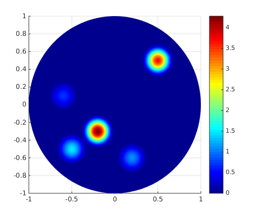
The physical parameters are chosen as follows. According to Assumption A-2, μr=1\mu_{r}=1. The frequency is selected such that ω^=π[cm1]\hat{\omega}=\pi[\text{cm}^{-1}], which corresponds to a frequency f=ω2π15f=\frac{\omega}{2\pi}\approx 15GHz. Density plots of εr\varepsilon_{r} and σ^\hat{\sigma} are displayed in Fig. 1. For εr\varepsilon_{r}, the background value is taken to be 37.2 for blood (see [18]) and there are 3 regions with smaller values of εr\varepsilon_{r} which are 7.79 (top) for fat, 20.2 (left) for nerve and 36.4 (right) for muscle. The source 𝐉^\hat{\mathbf{J}} is a real vector, whose components are shown in Fig. 2.


Refer to caption
Refer to caption
Figure 1. Left: εr\varepsilon_{r}, Right: σ^[cm1]\hat{\sigma}[\text{cm}^{-1}]
Refer to caption
Refer to caption
Figure 2. Source 𝐉^\hat{\mathbf{J}}. Left: xx-component, Right: yy-component.

Auxiliary solutions are needed in the reconstruction to compute the vector internal data (18) from the scalar internal data (17). Such solutions are obtained by solving the equation for j=1,2j=1,2:

××𝐅j(ω^2εr+iω^σ^)𝐅j=0in Ω,\nabla\times\nabla\times\mathbf{F}_{j}^{*}-(\hat{\omega}^{2}\varepsilon_{r}+i\hat{\omega}\hat{\sigma})\mathbf{F}_{j}^{*}=0\quad\text{in }\quad\Omega,

along with the impedance boundary condition

(1iω^×𝐅j)×𝐧^λ(𝐧^×𝐅j)×𝐧^=𝔤jon Ω.\left(\frac{1}{i\hat{\omega}}\nabla\times\mathbf{F}_{j}^{*}\right)\times\hat{\mathbf{n}}-\lambda(\hat{\mathbf{n}}\times\mathbf{F}_{j}^{*})\times\hat{\mathbf{n}}=\mathfrak{g}_{j}\quad\quad\text{on }\quad\partial\Omega.

where 𝔤k\mathfrak{g}_{k} is defined by

𝔤j:=1iω^×𝐄j×𝐧λ(𝐧×𝐄j)×𝐧 on Ω,\mathfrak{g}_{j}:=\frac{1}{i\hat{\omega}}\nabla\times\mathbf{E}_{j}\times\mathbf{n}-\lambda(\mathbf{n}\times\mathbf{E}_{j})\times\mathbf{n}\;\text{ on }\partial\Omega, (33)

with 𝐄1=(eiky,0)\mathbf{E}_{1}=(e^{-iky},0) and 𝐄2=(0,eikx)\mathbf{E}_{2}=(0,e^{-ikx}). Here the wave number k=(ω^2εr+iω^σ^)k=\sqrt{(\hat{\omega}^{2}\varepsilon_{r}+i\hat{\omega}\hat{\sigma})}, where εr,σ^\varepsilon_{r},\hat{\sigma} are taken from the background values corresponding to blood. The rationale for the choice of 𝔤j\mathfrak{g}_{j} is that when the medium is homogeneous, then 𝐄1\mathbf{E}_{1} and 𝐄2\mathbf{E}_{2} are mutually orthogonal plane waves. Clearly, such an orthogonality relation may not hold in practice due to the distortion caused by the inhomogeneity.

5.1. Case (I.1)

In this experiment, the modulation parameters are chosen as γJ=0\gamma_{J}=0, γε=0.25\gamma_{\varepsilon}=0.25, γσ=0.35\gamma_{\sigma}=0.35. The scalar internal data QQ is obtained by solving the forward problem (1). Then 0.1%0.1\% multiplicative noise is added to the signal. The vector internal data 𝐐\mathbf{Q} is calculated from the auxiliary solutions. The reconstruction is carried out using the procedure described in Proposition 4.1. That is, we solve for 𝐄\mathbf{E} from (18) and then recover 𝐉\mathbf{J} from the Maxwell equations (1) through the following weak formulation by setting δ=0\delta=0 in (3.2):

iω(𝐉,ϕ)(L2(Ω))3\displaystyle i\omega\left(\mathbf{J},\bm{\phi}\right)_{(L^{2}(\Omega))^{3}}
=(1μ×𝐄,×ϕ)(L2(Ω))3((ω2ε+iωσ)𝐄,ϕ)(L2(Ω))3iωλ𝐄T,ϕT.\displaystyle=\left(\frac{1}{\mu}\nabla\times\mathbf{E},\nabla\times\bm{\phi}\right)_{(L^{2}(\Omega))^{3}}-\left((\omega^{2}\varepsilon+i\omega\sigma)\mathbf{E},\bm{\phi}\right)_{(L^{2}(\Omega))^{3}}-i\omega\langle\lambda\mathbf{E}_{T},\bm{\phi}_{T}\rangle.

Here 𝐉\mathbf{J} is solved under the Galerkin framework by treating the left-hand side iω(𝐉,ϕ)(L2(Ω))3i\omega\left(\mathbf{J},\bm{\phi}\right)_{(L^{2}(\Omega))^{3}} as the bilinear form and the right-hand side as the linear form with known 𝐄\mathbf{E}. The reconstructed source is shown in Fig. 3.

Refer to caption
Refer to caption
Refer to caption
Refer to caption
Figure 3. Reconstructed source current vector for Case (I.1). Top row: from left to right, real part of the xx component and the yy component. Bottom row: from left to right, cross sections of the reconstruction and the true solution along the line y=xy=x. The relative L2L^{2} error of reconstruction is 32.5%32.5\%.

5.2. Case (II.4)

In this experiment, the modulation parameters are chosen as γJ=0.65\gamma_{J}=0.65, γε=0.35\gamma_{\varepsilon}=0.35, γσ=0.35\gamma_{\sigma}=0.35. The scalar internal data QQ is obtained by solving the forward problem (1). Then 1%1\% multiplicative noise is added to the signal. The vector internal data 𝐐\mathbf{Q} is found using the auxiliary solutions. The reconstruction is performed according to Proposition 4.3. That is, the boundary value problem (22), (3) is solved to obtain 𝐄\mathbf{E}. The Maxwell equations (1) are then used to find 𝐉\mathbf{J} through the similar approach of Case (I.1). The reconstructed source 𝐉^rec\hat{\mathbf{J}}_{rec} is shown in Fig. 4.

Refer to caption
Refer to caption
Refer to caption
Refer to caption
Figure 4. Reconstructed source current vector 𝐉^rec\hat{\mathbf{J}}_{rec} for Case 6. Top row: from left to right, real part of xx component and yy component. Bottom row: from left to right, cross sections of reconstruction and the true solution along the line y=xy=x. The relative L2L^{2} error of reconstruction is 3.2%3.2\%.
Remark 5.1.

The reconstructions for Case (II.4) are much better than those for Case (I.1). This can be explained by the corresponding stability estimates. Proposition 4.1 for Case (I.1) requires the H(curl)H(curl) norm of 𝐐\mathbf{Q} to be bounded, which is very sensitive to noise. In contrast, the stability estimate in Proposition 4.3 for Case (II.4) only requires that the L2L^{2} norm of 𝐐\mathbf{Q} be bounded.

6. Acknowledgments

The work of JCS was supported in part by the NSF grant DMS-1912821 and the AFOSR grant FA9550-19-1-0320. The work of YY is supported in part by the NSF grants DMS-1715178 and DMS-2006881.

References

  • [1] R. Albanese and P. Monk, The inverse source problem for Maxwell’s equations, Inverse Problems, 22 (2006), p. 1023.
  • [2] H. Ammari, E. Bonnetier, Y. Capdeboscq, M. Tanter, and M. Fink, Electrical impedance tomography by elastic deformation, SIAM J. Appl. Math, 68 (2008), p. 1557–1573.
  • [3] G. Bal, F. Chung, and J. Schotland, Ultrasound modulated bioluminescence tomography and controllability of the radiative transport equation. SIAM J. Math. Anal., 48 (2016), pp. 1332–1347.
  • [4] G. Bal and G. Uhlmann, Inverse diffusion theory of photoacoustics, Inverse Problems, 26 (2010), p. 085010.
  • [5] G. Bal, C. Guo, and F. Monard, Imaging of anisotropic conductivities from current densities in two dimensions, SIAM J. Imag. Sci., 7 (2014), pp. 2538–2557.
  • [6] G. Bal and J. Schotland, Inverse scattering and acousto-optic tomography, Phys. Rev. Lett., 104 (2010), p. 043902.
  • [7]  , Ultrasound-modulated bioluminescence tomography, Phys. Rev. E [Rapid Communication], 89 (2014), p. 031201.
  • [8] G. Bao, P. Li and Y. Zhao, Stability for the inverse source problems in elastic and electromagnetic waves, J. Math. Pure. Appl., 134 (2020) 122–178.
  • [9] N. Bleistein and J. Cohen, Nonuniqueness in the inverse source problem in acoustics and electromagnetics, J. Math. Phys., 18 (1977).
  • [10] Y. Capdeboscq, J. Fehrenbach, F. de Gournay, and O. Kavian, Imaging by modification: numerical reconstruction of local conductivities from corresponding power density measurements, SIAM J. Imag. Sci., 2 (2009).
  • [11] M. Cessenat, Mathematical Methods in Electromagnetism Linear Theory and Applications, World Scientific, 1996.
  • [12] F. Chung, J. Hoskins, and J. Schotland, Coherent acousto-optic tomography with diffuse light, Opt. Lett., 45 (2020), pp. 1623–1626.
  • [13] F. Chung, J. Hoskins, and J. Schotland, Radiative transport model for coherent acousto-optic tomography, Inverse Problems, 36 (2020), p. 064004.
  • [14] F. Chung and J. Schotland, Inverse transport and acousto-optic imaging, SIAM J. Math. Anal., 49 (2017), pp. 4704–4721.
  • [15] F. Chung, T. Yang, and Y. Yang, Ultrasound modulated bioluminescence tomography with a single optical measurement, Inverse Problems, 37 (2021), p. 015004.
  • [16] A. Devaney and E. Wolf, Radiating and nonradiating classical current distributions and fields they generate, Phys. Rev. D, 8 (1973), p. 1044.
  • [17] G. B. Folland, Introduction to Partial Differential Equations, Princeton University Press, 2 ed., 1995.
  • [18] C. Gabriel, Compilation of the dielectric properties of body tissues at RF and microwave frequencies., tech. rep., King’s Coll London (United Kingdom) Dept of Physics, 1996.
  • [19] A. Gebauer and O. Scherzer, Impedance-acoustic tomography, SIAM J. Appl. Math, 69 (2008), p. 565.
  • [20] V. Isakov, Inverse Source Problems, American Mathematical Society, 1990.
  • [21] M. Kempe, M. Larionov, D. Zaslavsky, and A. Genack, Acousto-optic tomography with multiply scattered light, JOSA A, 14 (1997), pp. 1151–1158.
  • [22] P. Kuchment and L. Kunyansky, 2d and 3d reconstructions in acousto-electric tomography, Inverse Problems, 27 (2011), p. 055013.
  • [23] P. Kuchment and D. Steinhauer, Stabilizing inverse problems by internal data, Inverse Problems, 28 (2012), p. 084007.
  • [24] W. Li, Y. Yang, and Y. Zhong, A hybrid inverse problem in the fluorescence ultrasound modulated optical tomography in the diffusive regime, SIAM J. Appl. Math., 79 (2019), pp. 356–376.
  • [25] W. Li, Y. Yang, and Y. Zhong, Inverse transport problem in fluorescence ultrasound modulated optical tomography with angularly averaged measurements, Inverse Problems, 36 (2020), p. 025011.
  • [26] W. Li, J. C. Schotland, Y. Yang, and Y. Zhong, An Acousto-electric inverse source problem, SIAM J. Imag. Sci., 14, 1601-1616 (2021)
  • [27] P. Monk, Finite Element Methods for Maxwell’s Equations, Oxford University Press, 2003.
  • [28] A. Nachman, A. Tamasan, and A. Timonov, Conductivity imaging with a single measurement of boundary and interior data., Inverse Problems., 23(6), (2007), p. 2551.
  • [29] R. Parmenter, The acousto-electric effect, Phys. Rev, 89 (1953), p. 990.
  • [30] R. Plonsey and R. Barr, Bioelectricity: A Quantitative Approach, Springer, 2007.
  • [31] J. Schotland, Acousto-optic imaging of random media, Prog. Opt, 65 (2020), pp. 347–380.
  • [32] F. Triki, Uniqueness and stability for the inverse medium problem with internal data, Inverse Problems, 26 (2010), p. 095014.
  • [33] Y. Zhao, G. Hu, P. Li, and X. Liu, Inverse source problems in electrodynamics, Inverse Problems and Imaging, 12 (2018), pp. 1411–1428.