Inverse properties of a class of pentadiagonal matrices related to higher order difference operators

Bakytzhan Kurmanbek Nazarbayev University, Department of Mathematics, 53 Kabanbay Batyr Ave, Nur-Sultan 010000, Kazakhstan Yogi Erlangga Zayed University, Department of Mathematics, Abu Dhabi Campus, P.O. Box 144534, United Arab Emirates Yerlan Amanbek Nazarbayev University, Department of Mathematics, 53 Kabanbay Batyr Ave, Nur-Sultan 010000, Kazakhstan Corresponding author

Abstract

This paper analyzes the convergence of fixed-point iterations of the form $\bm{u}=f(\bm{u})$ and the properties of the inverse of the related pentadiagonal matrices, associated with the fourth-order nonlinear beam equation. This nonlinear problem is discretized using the finite difference method with the clamped-free and clamped-clamped boundary conditions in the one dimension. Explicit formulas for the inverse of the matrices and norms of the inverse are derived. In iterative process, the direct computation of inverse matrix allows to achieve an efficiency. Numerical results were provided.

Keywords. explicit formula, pentadiagonal matrices, finite difference, nonlinear beam equation, fixed point method

1 Introduction

Many applications give arise to mathematical problems that involve numerical computations with pentadiagonal matrices, which require their inversion (see [1] and references therein). Even though inversion of a nonsingular pentadiagonal matrix can be done efficiently by a numerical linear algebra software, explicit inverse formulas are useful, for example, in a computer algebra software.

Early results on inverses of banded matrices can be traced as far back as to the work of [2, 3, 4] for general band matrices. Results for band Toeplitz matrices are given in [5], with explicit inverse formulas for tridiagonal matrices in [6, 7] and pentadiagonal matrices in [8, 9, 10, 1, 11, 12, 13]. In addition, properties including determinants of such matrices related to finite difference operators have been investigated, e.g. in [14, 15, 16].

In this study, we focus on the specific pentadiagonal matrices arising in a fixed-point iteration for numerically solving the fourth-order nonlinear beam equation:

\displaystyle\displaystyle\frac{d^{4}\widehat{\phi}}{d\widehat{x}^{4}}=\alpha_{1}e^{\displaystyle-\alpha_{2}\widehat{\phi}},\quad\widehat{x}\in\Omega=(0,L).

This nonlinear equation finds applications in mechanical and civil engineering, which models, e.g., a cantilever beam subjected to swelling pressure on one side. In the above equation, the right-hand side term is the swelling pressure, which in this form is proposed by Grob [17], based on empirical studies (see, e.g., [18] and the references therein), $L>0$ is the length of the beam, and $\alpha_{1},\alpha_{2}>0$ represents the mechanical property of the beam, which are assumed to be constant.

Scaling the domain to unity using the dimensionless variable $x=\widehat{x}/L$ and setting $\phi=\alpha_{2}\widehat{\phi}$ yields

\displaystyle\displaystyle\frac{d^{4}\phi}{dx^{4}}=Ke^{-\phi},\text{ in }\Omega=(0,1),

(1)

where $K=\alpha_{1}\alpha_{2}L>0$ . We shall use this formulation throughout. For (1) two types of boundary conditions are employed:

1.

Clamped-Free (CF) condition:

$\displaystyle\phi(0)=\phi^{\prime}(0)=0\quad\text{and}\quad\phi^{\prime\prime}(1)=\phi^{\prime\prime\prime}(1)=0,$ (2)
2.

Clamped-Clamped (CC) condition:

$\displaystyle\phi(0)=\phi^{\prime}(0)=0\quad\text{and}\quad\phi(1)=\phi^{\prime}(1)=0.$ (3)

Since $\displaystyle\frac{d^{4}\phi}{dx^{4}}=Ke^{-\phi}>0$ , obviously, $\phi=0$ can not be a solution, even though it satisfies the boundary conditions.

The solution of (1) with the boundary conditions (2) is concave up and an increasing function, which can be deduced from a mixed formulation of (2):

\begin{cases}\displaystyle\frac{d^{2}\omega}{dx^{2}}=Ke^{-\phi},&\omega(1)=\omega^{\prime}(1)=0,\\[10.0pt] \displaystyle\frac{d^{2}\phi}{dx^{2}}=\omega,&\phi(0)=\phi^{\prime}(0)=0.\\ \end{cases}

(4)

From the first part of (4), with $e^{-\phi}>0$ in $\Omega$ , $\omega^{\prime\prime}>0$ , and $w^{\prime}$ increases in $\Omega$ . The condition $\omega^{\prime}(1)=0$ requires that $w^{\prime}<0$ in $\Omega$ , which furthermore, together with the condition $\omega(1)=0$ , implies that $\omega>0$ and decreases. From the second part of (4), we have $\phi^{\prime\prime}=\omega>0$ ; thus, $\phi^{\prime}$ is an increasing function in $\Omega$ . Since $\phi^{\prime}(0)=0$ , $\phi>0$ , which implies $\phi>0$ and increases. This characterization also holds in the finite-difference setting based on the second-order scheme we use in this paper (c.f. Section 4).

Numerical methods based on finite element methods for (1) have been proposed and studied, e.g., in [19, 20], where focus is given on the accurate approximation of the solution. This paper approaches the problem from a different angle, with emphasis put on the convergence of the iteration method of the form

\phi=\mathcal{L}^{-1}\left(Ke^{-\phi}\right),

where $\mathcal{L}=d^{4}/dx^{4}$ , and the properties of the related iteration matrices involved. Using the second-order finite difference approach, these matrices are pentadiagonal and near Toeplitz.

In this paper, we present explicit formulas for inverses of the specific pentadiagonal matrices and their bounds of norms, which are necessary in the convergence analysis of the fixed-point iteration. As the inverse can be formed explicitly, we are able to construct an exact norm of some of those matrices. The convergence rate for the clamped-free and clamped-clamped problems were derived and then numerical examples were presented for different parameters.

The paper is organized as follows. Section 2 is devoted to the convergence and the inverse of the iteration matrix for problem with the clamp-free condition. Similar discussion for the clamp-clamp condition is given in Section 3. Numerical results are presented in Section 4, followed by some concluding remarks in Section 5.

2 The case with clamped-free boundary conditions

We consider $n+1$ equidistant grid points on the closed interval $[0,1]$ , with the distance (grid size) $h=1/n$ , at which the solution of (1) is approximated by a finite difference scheme. Each grid point is indexed by $i=0,\dots,n$ , where $i=0$ and $n$ correspond to the boundary points. Throughout the paper, we shall consider $n\geq 5$ for $A$ to be a meaningful approximation to the differential operator $\mathcal{L}$ , even though $n=5$ may not be of practical interest.

For the interior nodes, $1\leq i\leq n-1$ , the fourth-order derivative is approximated by the second-order finite difference scheme:

\frac{d^{4}\phi}{dx^{4}}(x_{i})\approx\frac{1}{h^{4}}(\phi_{i-2}-4\phi_{i-1}+6\phi_{i}-4\phi_{i+1}+\phi_{i+2}),

where $x_{i}=ih$ and $\phi_{i}\equiv\phi(x_{i})$ . For $i=2$ , we just impose the boundary condition $\phi(0)\equiv\phi_{0}=0$ . For $i=1$ , $\phi_{-1}$ corresponds to a fictitious point outside the computational domain, which is eliminated using the central scheme approximation to the boundary condition $\phi^{\prime}(0)=0$ . Similar approaches are used for $i=n-1$ and $n$ , with the boundary conditions $\phi^{\prime\prime}(1)=\phi^{\prime\prime\prime}(1)=0$ be approximated by appropriate second-order finite difference schemes.

The resultant system of nonlinear equations is

\displaystyle A\bm{u}=h^{4}K\exp(\bm{-u}),

(5)

where $\bm{u}=(u_{1},\dots,u_{n})^{T}\in\mathbb{R}^{n}$ , with $u_{i}\approx\phi(x_{i})$ , and

\displaystyle A:=\left[\begin{array}[]{rrrrrrr}7&-4&1&0&\cdots&&0\\ -4&6&-4&\ddots&\ddots&&\vdots\\ 1&-4&\ddots&\ddots&&&\\ 0&\ddots&\ddots&&\ddots&1&0\\ &\ddots&&\ddots&6&-4&1\\ \vdots&&&1&-4&5&-2\\ 0&\cdots&&0&2&-4&2\end{array}\right].

(13)

Here, $A\in\mathbb{R}^{n\times n}$ is a nonsymmetric, nondiagonally dominant pentadiagonal matrix.

Our first result on $A$ is that it is nonsingular. In fact, we have the following theorem of the explicit inverse of matrix

Theorem 2.1.

Let $B=[b_{i,j}]_{i,j=1,n}\in\mathbb{R}^{n\times n}$ such that

	$\displaystyle b_{i,j}$	$\displaystyle=\displaystyle\frac{3ij^{2}+j-j^{3}}{6},\quad\forall j\leq i,i\in\{1,2,\dots,n\},j\in\{1,2,\dots,n-1\},$
	$\displaystyle b_{i,n}$	$\displaystyle=\frac{1}{2}b_{n,i},$
	$\displaystyle b_{n,n}$	$\displaystyle=\frac{1}{12}n(2n^{2}+1),$
	$\displaystyle b_{i,j}$	$\displaystyle=b_{j,i},\quad i,j\in\{1,2,\dots,n-1\}.$

Then $B$ is the inverse of $A$ , where $A=[a_{i,j}]_{i,j=1,n}$ is given in (13).

Proof.

The proof is done by the direct computation. Let $D$ be matrix such that $D=AB$ . We want to show that the product

d_{i,j}:=\left[a_{i,1}\,\,a_{i,2}\,\,\cdots\,\,a_{i,n}\right]\left[\begin{array}[]{c}b_{1,j}\\ b_{2,j}\\ \vdots\\ b_{n,j}\end{array}\right]=\begin{cases}1,&i=j,\\ 0,&i\neq j.\end{cases}

In other words, $D$ is the identity matrix $n\times n$ .

(i)

The case $3\leq i\leq n-2$ and $1\leq j\leq n$ .

In this case, $a_{i,i-2}=1$ , $a_{i,i-1}=-4$ , $a_{i,i}=6$ , $a_{i,i+1}=-4$ , $a_{i,i+2}=1$ , while the others are $0$ . Therefore,

$d_{i,j}=b_{i-2,j}-4b_{i-1,j}+6b_{i,j}-4b_{i+1,j}+b_{i+2,j}.$ (14)

If $i=j$ , then $b_{i-2,i}=b_{i,i-2}=(2i^{3}-6i^{2}+i+6)/6$ , $b_{i-1,i}=b_{i,i-1}=(2i^{3}-3i^{2}+i)/6$ , $b_{ii}=(2i^{3}+i)/6$ , $b_{i+1,i}=(2i^{3}+3i^{2}+i)/6$ , and $b_{i+2,i}=(2i^{3}+6i^{2}+i)/6$ , yielding $d_{i,i}=1$ .
For $i\neq j$ , we consider several cases.
1. (a)
  
  $j\leq i-2$ ; Then $b_{i-2,j}=(3ij^{2}+j-6j^{2}-j^{3})/6$ , $b_{i-1,j}=(3ij^{2}+j-3j^{2}-j^{3})/6$ , $b_{i,j}=(3ij^{2}+j-j^{3})/6$ , $b_{i+1,j}=(3ij^{2}+j+3j^{2}-j^{3})/6$ , $b_{i+2,j}=(3ij^{2}+j+6j^{2}-j^{3})/6$ , yielding $d_{i,j}=0$ .
2. (b)
  
  $j=i-1$ ; Then $b_{i-2,j}=(2i^{3}-9i^{2}+13i-6)/6$ , $b_{i-1,j}=(2i^{3}-6i^{2}+7i-3)/6$ , $b_{i,j}=(2i^{3}-3i^{2}+i)/6$ , $b_{i+1,j}=(2i^{3}-5i+3)/6$ , $b_{i+2,j}=(2i^{3}+3i^{2}-11i+6)/6$ , yielding $d_{i,i-1}=0$ ;
3. (c)
  
  $j=i+1$ ; Then $b_{i-2,j}=b_{j,i-2}=(2i^{3}-3i^{2}-11i+18)/6$ , $b_{i-1,j}=b_{j,i-1}=(2i^{3}-5i+3)/6$ , $b_{i,j}=b_{j,i}=(2i^{3}+3i^{2}+i)/6$ , $b_{i+1,j}=(2i^{3}+6i^{2}+7i+3)/6$ , $b_{i+2,j}=(2i^{3}+9i^{2}+13i+6)/6$ , yielding $d_{i,i+1}=0$ .
4. (d)
  
  $j\geq i-1$ ; Then $b_{i-2,j}=b_{j,i-2}=(3j(i-2)^{2}+(i-2)-(i-2)^{3})/6$ , $b_{i-1,j}=b_{j,i-1}=(3j(i-1)^{2}+(i-1)-(i-1)^{3})/6$ , $b_{i,j}=b_{j,i}=\frac{3ji^{2}+i-i^{3}}{6}$ , $b_{i+1,j}=(3j(i+1)^{2}+(i+1)-(i+1)^{3})/6$ , $b_{i+2,j}=(3j(i+2)^{2}+(i+2)-(i+2)^{3})/6$ , yielding $d_{i,j}=0$ .
(ii)

The case $i=1$ .

For $j=1$ , $b_{1,1}=3/6$ , $b_{2,1}=1$ , and $b_{3,1}=3/2$ ; Thus, $d_{i,j}=d_{1,1}=7b_{1,1}-4b_{2,1}+b_{3,1}=1$ .

For $j>1$ , we have $b_{1,j}=b_{j,1}=j/2$ , $b_{2,j}=b_{j,2}=2j-1$ , and $b_{3,j}=b_{j,3}=\frac{9j}{2}-4$ ; Thus, $d_{i,j}=7b_{1,j}-4b_{2,j}+b_{3,j}=0$ .
(iii)

The case $i=2$ , with ${d_{i,j}}=-4b_{1,j}=6b_{2,j}-4b_{3,j}+b_{4,j}$ .

For $j=2$ , we have $b_{1,2}=b_{2,1}=1$ , $b_{2,2}=3$ , $b_{3,2}=5$ , $b_{4,2}=7$ ; Thus, $d_{2,2}=1$ .

For $j\neq 2$ , then $b_{1,j}=j/2$ , $b_{2,j}=2j-1$ , $b_{3,j}=\frac{9j}{2}-4$ , and $b_{4,j}=8j-10$ . We have $d_{i,j}=0$ .
(iv)

For the case $i\in\{n-1,n\}$ , similar computations using (14) complete the proof.

∎

From now on, we shall use $a_{i,j}^{-1}$ to denote the $(i,j)$ -entry of $A^{-1}$ , the inverse of $A$ ; thus, $a^{-1}_{i,j}=b_{i,j}$ .

The following corollary is a consequence of Theorem 2.1.

Corollary 2.2.

The inverse of $A$ is a positive matrix; i.e., $A^{-1}>0$ , implying $a^{-1}_{i,j}>0$ .

Proof.

By Theorem 2.1 it follows that $a^{-1}_{n,n}=n(2n^{2}+1)/12$ is positive. Notice that, for $i\geq j$ , $a_{i,j}^{-1}=\displaystyle\frac{3ij^{2}+j-j^{3}}{6}\geq\frac{3j^{3}+j-j^{3}}{6}>0$ . Consequently, entries determined by the other 2 parts of Theorem 2.1 are also positive. ∎

The above positivity result is important in the context of the fixed-point iteration we devise to solve the nonlinear system (5). Consider the iteration

\displaystyle\bm{u}^{\ell}=h^{4}KA^{-1}\exp(-\bm{u}^{\ell-1}),\ell=1,2.\dots

(15)

Since $A^{-1}>0$ (Corollary 2.2), the recipe (15) generates a sequence of positive vectors $\{\bm{u}^{\ell}\}$ , if started with $\bm{u}^{0}>\bm{0}$ . As the solution of this type of boundary-value problem is a nonnegative function (c.f., Section 1; see also later for the finite-difference equation case), if the above iteration converges, it converges to a positive solution.

Let $p\in\{1,2,\infty\}$ . Our starting point for the convergence analysis is the relation, with $\bm{u}^{0}>\bm{0}$ ,

	$\displaystyle\\|\bm{u}^{\ell}-\bm{u}^{\ell-1}\\|_{p}$	$\displaystyle=\\|h^{4}KA^{-1}(\exp(-\bm{u}^{\ell-1})-\exp(-\bm{u}^{\ell-2}))\\|_{p}$
		$\displaystyle=h^{4}K\\|A^{-1}\left(\exp(-\bm{u}^{\ell-2})+G(\bm{u}^{\ell-1}-\bm{u}^{\ell-2})-\exp(-\bm{u}^{\ell-2})\right)\\|_{p}$
		$\displaystyle=h^{4}K\\|A^{-1}G(\bm{u}^{\ell-1}-\bm{u}^{\ell-2})\\|_{p},$

where $G=-\text{diag}(\exp(-\xi_{1}),\dots,\exp(-\xi_{n}))$ , such that the vector $\bm{\xi}=[\xi_{i}]_{i=1,n}\in\mathcal{B}=\{\bm{x}\in\mathbb{R}^{n}:\|\bm{x}-\bm{u}^{\ell-2}\|_{p}<\|\bm{u}^{\ell-1}-\bm{u}^{\ell-2}\|_{p}\}$ . Since $\{\bm{u}^{\ell}\}$ is a sequence of positive vectors, $\bm{\xi}$ is also a positive vector, and consequently the diagonal entries of $G$ are strictly less than 1. Thus, $\|G\|_{p}<1$ , and

	$\displaystyle\\|\bm{u}^{\ell}-\bm{u}^{\ell-1}\\|_{p}$	$\displaystyle\leq$	$\displaystyle h^{4}K\\|A^{-1}\\|_{p}\\|G\\|_{p}(\bm{u}^{\ell-1}-\bm{u}^{\ell-2})\\|_{p}$		(16)
		$\displaystyle<$	$\displaystyle h^{4}K\\|A^{-1}\\|_{p}\\|\bm{u}^{\ell-1}-\bm{u}^{\ell-2}\\|_{p}.$		(16)

We define $L_{p}$ to be

L_{p}=h^{4}K\|A^{-1}\|_{p}.

(17)

Convergence guarantee of the fixed point iteration (15) requires $L_{p}<1$ , which in turn, for given $K$ and chosen $h$ , requires that

\|A^{-1}\|_{p}<1/(h^{4}K).

(18)

Lemma 2.3.

For the inverse of $A$ in Theorem 2.1, the following holds true:

a_{i_{1},j}^{-1}>a_{i_{2},j}^{-1},\quad\forall i_{1}>i_{2}>j,\text{ with }i_{1},i_{2},j\in\{1,2,\dots,n\}.

Proof.

From Theorem 2.1 it follows that $a^{-1}_{i_{1},j}=(3i_{1}j^{2}+j-j^{3})/6$ and $a_{i_{2},j}^{-1}=(3i_{2}j^{2}+j-j^{3})/6$ , thus, one can notice that $a_{i_{1},j}^{-1}>a_{i_{2},j}^{-1}$ , for $i_{1}>i_{2}>j$ . ∎

Theorem 2.4.

Let $A\in\mathbb{R}^{n\times n}$ be given in (13), with $n\geq 5$ . Then

\|A^{-1}\|_{p}=\begin{cases*}(n^{4}-n^{2})/8,\quad\text{if }p=1,\\[5.0pt] (n^{4}+n^{2})/8,\quad\text{if }p=\infty.\end{cases*}

Proof.

For $p=1$ case, it follows from Lemma 2.3 that

\|A^{-1}\|_{1}=\max_{1\leq j\leq n}\sum_{i=1}^{n}|a_{i,j}^{-1}|=\max\left\{\sum_{i=1}^{n}|a^{-1}_{i,n-1}|,\sum_{i=1}^{n}|a^{-1}_{i,n}|\right\}.

We have

\sum_{i=1}^{n}|a_{i,n-1}^{-1}|=\sum_{i=1}^{n}|a_{n-1,i}^{-1}|=\sum_{i=1}^{n}\frac{3(n-1)i^{2}+i-i^{3}}{6}=\frac{n^{4}-n^{2}}{8}.

We can now proceed similarly:

\sum_{i=1}^{n}|a_{i,n}^{-1}|=\frac{1}{2}\sum_{i=1}^{n}|a_{n,i}^{-1}|=\frac{1}{2}\sum_{i=1}^{n}\frac{3ni^{2}+i-i^{3}}{6}=\frac{3n^{4}+4n^{3}+3n^{2}+2n}{48}.

From the above results,

\sum_{i=1}^{n}|a_{i,n-1}^{-1}|-\sum_{i=1}^{n}|a_{i,n}^{-1}|=\frac{3n^{4}-4n^{3}-9n^{2}-2n}{48}>0

for $n\geq 5$ . Therefore,

\max_{1\leq j\leq n}\sum_{i=1}^{n}|a_{i,j}^{-1}|\leq\sum_{i=1}^{n}|a_{i,n-1}^{-1}|=\frac{n^{4}-n^{2}}{8}=\|A^{-1}\|_{1}.

Next for $p=\infty$ using the Lemma 2.3,

$\displaystyle\\|A^{-1}\\|_{\infty}$	$\displaystyle=$	$\displaystyle\max_{1\leq i\leq n}\sum_{j=1}^{n}\|a_{i,j}^{-1}\|=\sum_{j=1}^{n}\|a_{n,j}^{-1}\|=\sum_{j=1}^{n-1}\|a_{n,j}^{-1}\|+a_{n,n}^{-1}$
	$\displaystyle=$	$\displaystyle\sum_{j=1}^{n-1}\frac{3nj^{2}+j-j^{3}}{6}+\frac{n(2n^{2}+1)}{12}$
	$\displaystyle=$	$\displaystyle\frac{n^{4}+n^{2}}{8}.$

∎

Using Hölder’s inequality,

\|A^{-1}\|_{2}\leq\sqrt{\|A^{-1}\|_{1}\|A^{-1}\|_{\infty}}=\frac{1}{8}\sqrt{n^{8}-n^{4}}\leq\frac{1}{8}n^{4}.

We conclude this section by the characterization of the finite difference solution of the system (5). Because $A\bm{u}=h^{4}K\exp(-\bm{u})>\bm{0}$ , for the last row of the system,

\displaystyle 2u_{n-2}-4u_{n-1}+2u_{n}>0\quad\Longrightarrow\quad u_{n}-u_{n-1}>u_{n-1}-u_{n-2}.

(19)

From the $(n-1)$ -th row, with $u_{n-3}-4u_{n-2}+5u_{n-1}-2u_{n}>0$ , we have

\displaystyle u_{n-1}-u_{n-2}>u_{n-2}-u_{n-3}+2u_{n-2}-4u_{n-1}+2u_{n}>u_{n-2}-u_{n-3},

(20)

after using the inequality (19). Furthermore, this row leads to

4(u_{n-1}-u_{n-2})>u_{n}-u_{n-3}+u_{n}-u_{n-1}>u_{n}-u_{n-3}+u_{n-1}-u_{n-2},

after again using (19), which in turn yields

\displaystyle 3(u_{n-1}-u_{n-2})>u_{n}-u_{n-3}.

(21)

We then have the following lemma:

Lemma 2.5.

For the inequality $A\bm{u}>\mathbf{0}$ , with $A$ given by (13), the following inequalities hold, with $j=i+2$ and $i=3\dots,n-1$ the rows of $A$ :

u_{j+2}-u_{j+1}>u_{j+1}-u_{j},\quad 3(u_{j+2}-u_{j+1})>u_{j+3}-u_{j}.

Proof.

We have proved the inequalities for $j=n-3$ , which comes from the $(n-1)$ -th row of $A\bm{u}>\mathbf{0}$ . Now suppose that they hold also for $j=n-3,n-4,\dots,k+1$ . Associated with $j=k$ is the inequality $u_{k}-4u_{k+1}+6u_{k+2}-4u_{k+3}+u_{k+4}>0$ from the $(k+2)$ -th row of $A\bm{u}>\mathbf{0}$ , which gives

$\displaystyle u_{k+2}-u_{k+1}$	$\displaystyle>$	$\displaystyle 3u_{k+1}-u_{k}-5u_{k+2}+4u_{k+3}-u_{k+4}$
	$\displaystyle=$	$\displaystyle u_{k+1}-u_{k}+\left[4(u_{k+3}-u_{k+2})+u_{k+1}-u_{k+4}+u_{k+1}-u_{k+2}\right]$
	$\displaystyle>$	$\displaystyle u_{k+1}-u_{k}+\left[3(u_{k+3}-u_{k+2})+u_{k+1}-u_{k+4}\right]$
	$\displaystyle>$	$\displaystyle u_{k+1}-u_{k}$

by assumption. Next, note that $u_{k}-4u_{k+1}+6u_{k+2}-4u_{k+3}+u_{k+4}=3(u_{k+2}-u_{k+1})+u_{k}-u_{k+3}-[3(u_{k+3}-u_{k+2})+u_{k+1}-u_{k+4}]>0$ . Thus, $3(u_{k+2}-u_{k+1})+u_{k}-u_{k+3}>3(u_{k+3}-u_{k+2})+u_{k+1}-u_{k+4}>0$ , by assumption. ∎

Theorem 2.6.

The solution of the finite difference system (5) is a nonnegative vector $\bm{u}$ , with increasing $u_{i}$ .

Proof.

On the nodes $i=0,1$ , approximation to the differential term leads to

u_{i-2}-4u_{i-1}+6u_{i}-4u_{i+1}+u_{i+2}>0,

which is of the same structure as the $i=3,\dots,n-2$ rows of $A$ . By Lemma 2.5,

u_{2}-u_{1}>u_{1}-u_{0},\quad u_{1}-u_{0}>u_{0}-u_{-1}.

Therefore,

u_{n}-u_{n-1}>u_{n-1}-u_{n-2}>\cdots>u_{2}-u_{1}>u_{1}-u_{0}>u_{0}-u_{-1}.

With $u_{0}=0$ (from the boundary condition $\phi(0)=\phi_{0}=0)$ and $u_{-1}=u_{1}$ (from using central finite differencing on $\phi^{\prime}(0)=0$ ), from the most right inequality, we get $u_{1}>0=u_{0}$ . Also, $u_{2}-u_{1}>u_{1}-u_{0}>0$ ; thus $u_{2}>u_{1}$ . In general, we have $u_{i+1}>u_{i}$ , $i=1,\dots,n-1$ . ∎

3 The case with clamped-clamped boundary conditions

In this section, we consider the case with the boundary conditions (3). Conditions at $x=1$ are treated in the same way as at $x=0$ , leading to (5), but now with $\bm{u}=(u_{1},\dots,u_{n-1})^{T}\in\mathbb{R}^{n-1}$ and $A\in\mathbb{R}^{(n-1)\times(n-1)}$ given by

\displaystyle A=\left[\begin{array}[]{rrrrrrr}7&-4&1&0&&\cdots&0\\ -4&6&-4&\ddots&\ddots&&\vdots\\ 1&-4&\ddots&\ddots&&\ddots&\\ 0&\ddots&\ddots&&\ddots&\ddots&0\\ &\ddots&&&\ddots&-4&1\\ \vdots&&\ddots&\ddots&-4&6&-4\\ 0&\cdots&&0&1&-4&7\end{array}\right].

(29)

However, to simplify our notation, we shall consider the case where $\bm{u}\in\mathbb{R}^{n}$ and $A\in\mathbb{R}^{n\times n}$ in the subsequent analysis; in this case, $h=1/(n+1)$ .

In constrast to (13), the matrix (29) is centrosymmetric and near Toeplitz. Furthermore, it admits the rank-2 decomposition as follows:

\displaystyle A=T^{2}+UU^{t},

(30)

where $T=\text{tridiag}_{n}(-1,2,-1)$ is an $n\times n$ tridiagonal symmetric Toeplitz matrix, and

\displaystyle U=\left[\begin{array}[]{cc}\sqrt{2}&0\\ 0&0\\ \vdots&\vdots\\ 0&\sqrt{2}\end{array}\right]\in\mathbb{R}^{n\times 2}.

(35)

$T$ is a symmetric M-matrix, with positive inverse given explicitly by (see, e.g., [10])

\displaystyle[T^{-1}]_{ij}=\begin{cases}\frac{j}{n+1}(n-(i-1)),&i\geq j,\\[5.0pt] \frac{i}{n+1}(n-(j-1)),&i<j.\end{cases}

(36)

$A$ is symmetric positive definite because $T^{2}=T^{T}T$ (and $UU^{t}$ ) is symmetric positive (semi) definite. The inverse of $A$ can be computed by applying the Sherman-Morrison formula on (30):

$\displaystyle A^{-1}$	$\displaystyle=T^{-2}-T^{-2}U(I_{2}+U^{t}T^{-2}U)^{-1}U^{t}T^{-2}$
	$\displaystyle=T^{-1}(I-T^{-1}U(I_{2}+U^{t}T^{-2}U)^{-1}U^{t}T^{-1})T^{-1}$
	$\displaystyle=T^{-t}(I-T^{-1}U(I_{2}+U^{t}T^{-2}U)^{-1}(T^{-1}U)^{t})T^{-1}.$	(37)

Because $A^{-1}$ is symmetric positive definite, the middle term on the right-hand side $I-T^{-1}U(I_{2}+U^{T}T^{-2}U)(T^{-1}U)^{T}$ is also symmetric positive definite. Rewriting (30) as

A=T^{2}+UU^{t}=T^{t}(I+T^{-1}U(T^{-1}U)^{t})T,

clearly

(I+T^{-1}U(T^{-1}U)^{t})^{-1}=I-T^{-1}U(I_{2}+U^{t}T^{-2}U)^{-1}(T^{-1}U)^{t}=:M.

Note that, with (35) and (36),

\displaystyle T^{-1}U=\frac{\sqrt{2}}{n+1}\left[\begin{array}[]{cc}n&1\\ n-1&2\\ \vdots&\vdots\\ 2&n-1\\ 1&n\end{array}\right].

(43)

Direct computation yields

	$\displaystyle I_{2}+U^{t}T^{-2}U$	$\displaystyle=$	$\displaystyle\frac{2}{(n+1)^{2}}\left[\begin{array}[]{ccc}\displaystyle\frac{(n+1)^{2}}{2}+\sum_{k=1}^{n}k^{2}&&\displaystyle\sum_{k=1}^{n}(n-(k-1))k\\ &&\\ \displaystyle\sum_{k=1}^{n}(n-(k-1))k&&\displaystyle\frac{(n+1)^{2}}{2}+\sum_{k=1}^{n}k^{2}\end{array}\right]$		(47)
		$\displaystyle=$	$\displaystyle\frac{1}{\gamma}\left[\begin{array}[]{ccc}\displaystyle\gamma+\tau&&\displaystyle\gamma n-\tau\\ &&\\ \displaystyle\gamma n-\tau&&\displaystyle\gamma+\tau\end{array}\right],$		(51)

where $\tau=\frac{2n^{3}+3n^{2}+n}{6}$ and $\gamma=\frac{(n+1)^{2}}{2}$ . Its inverse is given by

\displaystyle(I_{2}+U^{T}T^{-2}U)^{-1}=\frac{1}{\delta}\left[\begin{array}[]{ccc}\displaystyle\gamma+\tau&&\displaystyle-\gamma n+\tau\\ &&\\ \displaystyle-\gamma n+\tau&&\displaystyle\gamma+\tau\end{array}\right],

(55)

where $\det(I_{2}+U^{T}T^{-2}U)=\frac{1}{3}(n^{2}+2n+3)>0$ and $\delta=(n+1)(2\tau+\gamma(1-n))=\frac{1}{6}(n+1)^{2}(n^{2}+2n+3)$ .

Let $M=[m_{ij}]_{i,j=1,n}$ . Using (43) and (55), we have, for $i\neq j$ ,

	$\displaystyle m_{ij}$	$\displaystyle=$	$\displaystyle-\frac{2}{\delta(n+1)^{2}}[n-(i-1)\quad i]\left[\begin{array}[]{ccc}\displaystyle\gamma+\tau&&\displaystyle-\gamma n+\tau\\ &&\\ \displaystyle-\gamma n+\tau&&\displaystyle\gamma+\tau\end{array}\right]\left[\begin{array}[]{c}n-(j-1)\\ j\end{array}\right]$
		$\displaystyle=$	$\displaystyle q_{0}(n)+q_{1}(n)(i+j)+q_{2}(n)ij,$

where

$\displaystyle q_{0}(n)$	$\displaystyle=$	$\displaystyle-\frac{4n^{2}+8n+6}{(n+1)(n^{2}+2n+3)},$
$\displaystyle q_{1}(n)$	$\displaystyle=$	$\displaystyle\frac{6}{n^{2}+2n+3},$
$\displaystyle q_{2}(n)$	$\displaystyle=$	$\displaystyle-\frac{12}{(n+1)(n^{2}+2n+3)}.$

One can verify that $m_{ij}$ change signs. Thus $M$ is not an M-matrix.

For $i=j$ ,

$\displaystyle m_{ii}$	$\displaystyle=$	$\displaystyle 1-\frac{2}{\delta(n+1)^{2}}[n-(i-1)\quad i]\left[\begin{array}[]{ccc}\displaystyle\gamma+\tau&&\displaystyle-\gamma n+\tau\\ &&\\ \displaystyle-\gamma n+\tau&&\displaystyle\gamma+\tau\end{array}\right]\left[\begin{array}[]{c}n-(i-1)\\ i\end{array}\right]$
	$\displaystyle=$	$\displaystyle\frac{n^{3}-n^{2}-3n-3}{(n+1)(n^{2}+2n+3)}+\frac{12}{n^{2}+2n+3}i-\frac{12}{(n+1)(n^{2}+2n+3)}i^{2}$
	$\displaystyle>$	$\displaystyle 0,$

for $n\geq 1$ .

Theorem 3.1.

The inverse of $A$ given by (29) is a positive matrix. Furthermore, let $\alpha=n+1-i$ , $\beta=j\alpha/(6(n+1)(n^{2}+2n+3))$ , and $\varepsilon=3(1+\alpha(n+1))(1+(i-j)j)$ . The entries of $A^{-1}$ are

•

$a^{-1}_{ij}=\beta(\varepsilon+(j^{2}-1)(2\alpha^{2}+1))$ , for $i\geq j$
•

$a^{-1}_{ij}=a^{-1}_{ji}$ , otherwise.

Proof.

Let $A^{-1}=[a^{-1}_{ij}]$ , with $A^{-1}=T^{-1}MT^{-1}$ . Denote by $\mathbf{y}_{j}=[y_{k,j}]_{k=1,n}=MT_{j}^{-1}$ , the product of $M$ and the $j$ -th column of $T^{-1}$ . For $i\geq j$ ,

\displaystyle\mathbf{y}_{j}=\frac{1}{n+1}\begin{bmatrix}(n+1-j)(m_{1,1}+2m_{1,2}+\cdots+jm_{1,j})+j(m_{1,j+1}(n-j)+\cdots+m_{1,n})\\ \vdots\\ (n+1-j)(m_{j,1}+2m_{j,2}+\cdots+jm_{j,j})+j(m_{j,j+1}(n-j)+\cdots+m_{j,n})\\ \vdots\\ (n+1-j)(m_{n,1}+2m_{n,2}+\cdots+jm_{n,j})+j(m_{n,j+1}(n-j)+\cdots+m_{n,n})\end{bmatrix}.

Using $m_{i,j}$ , for $i\leq j$ , we have, with $m^{*}_{i,j}=q_{0}+q_{1}(i+j)+q_{2}ij$ ,

$\displaystyle y_{i,j}$	$\displaystyle=$	$\displaystyle\frac{(n-(j-1))i}{n+1}$
	$\displaystyle+$	$\displaystyle\frac{n+1-j}{n+1}(m^{}_{i,1}+2m^{}_{i,2}+\cdots+jm^{}_{i,j})+\frac{j}{n+1}(m^{}_{i,j+1}(n-j)+\cdots+m^{*}_{i,n})$
	$\displaystyle=$	$\displaystyle\frac{(n-(j-1))i}{n+1}$
	$\displaystyle+$	$\displaystyle\frac{q_{0}+q_{1}i}{n+1}((n+1-j)(1+\cdots+j)+j(n-j+\cdots+1))$
	$\displaystyle+$	$\displaystyle\frac{q_{1}+q_{2}i}{n+1}((n+1-j)(1^{2}+\cdots+j^{2})+j((n-j)(j+1)+(n-j-1)(j+2)+\cdots+n))$
	$\displaystyle=$	$\displaystyle\frac{1}{n+1}\left((n-(j-1))i+r_{0}+r_{1}i\right),$

where

r_{0}=-\frac{j(n+1-j))((n+1)(n+1-j)+1)}{n^{2}+2n+3}

and

r_{1}=\frac{j(n+1-j)(n+1-2j)}{n^{2}+2n+3}.

Using similar calculation for $i>j$ , we get

y_{i,j}=\frac{1}{n+1}\begin{cases}\displaystyle r_{0}+r_{1}i+(n+1-j)i=r_{0}+\left(r_{1}-j\right)i+(n+1)i,&i\leq j,\\ \displaystyle r_{0}+r_{1}i+(n+1-i)j=r_{0}+\left(r_{1}-i\right)i+(n+1)j,&i>j;\end{cases}

hence,

\mathbf{y}_{j}=\frac{1}{n+1}\left(r_{0}\begin{bmatrix}1\\ \vdots\\ 1\\ 1\\ \vdots\\ 1\end{bmatrix}+\left(r_{1}-j\right)\begin{bmatrix}1\\ \vdots\\ j-1\\ j\\ \vdots\\ n\end{bmatrix}+(n+1)\begin{bmatrix}1\\ \vdots\\ j-1\\ j\\ \vdots\\ j\end{bmatrix}\right).

Consider the $i$ -th row of $T^{-1}$ :

T_{i}^{-t}=\frac{1}{n+1}\begin{bmatrix}n+1-i&2(n+1-i)&\cdots&i(n+1-i)&i(n-i)&\cdots&i\end{bmatrix}.

We have

$\displaystyle a^{-1}_{ij}$	$\displaystyle=$	$\displaystyle T_{i}^{-t}MT_{j}^{-1}=T_{i}^{-t}\mathbf{y}_{j}$
	$\displaystyle=$	$\displaystyle r_{0}\frac{i(n+1-i)}{2}+\left(r_{1}-\frac{j}{n+1}\right)\frac{i(n+1-i)(n+1+i)}{6}$
	$\displaystyle+$	$\displaystyle\frac{j(n+1-i)(3i(n+1)+1-j^{2})}{6(n+1)}$
	$\displaystyle=$	$\displaystyle\beta(\varepsilon+(j^{2}-1)(2\alpha^{2}+1)),$

where

$\displaystyle\alpha$	$\displaystyle=$	$\displaystyle\displaystyle{n+1-i},$
$\displaystyle\beta$	$\displaystyle=$	$\displaystyle\displaystyle\frac{j(n+1-i)}{6(n+1)(n^{2}+2n+3)},$
$\displaystyle\varepsilon$	$\displaystyle=$	$\displaystyle\displaystyle{3(1+\alpha+n\alpha)(1+ij-j^{2})}.$

Notice that $\alpha,\beta,\varepsilon>0$ , $\forall i,j=1,\dots,n$ . With $i\geq j$ and $j^{2}>j^{2}-1$ ,

	$\displaystyle a_{ij}^{-1}$	$\displaystyle>$	$\displaystyle\beta(j^{2}-1)(2\alpha^{2}+1)$
		$\displaystyle\geq$	$\displaystyle 0.$

∎

By Theorem 3.1, starting from $\bm{u}^{0}>\bm{0}$ , the fixed-point iteration (15) is guaranteed to generate a sequence of positive vectors.

In the sequel, we present two ways of constructing an estimate for norms of the inverse of $A$ . The first approach is based on the factorization $A^{-1}=T^{-t}M^{-1}T^{-1}$ in (37). The result is presented in the next theorem.

Theorem 3.2.

For $p\in\{1,2,\infty\}$ ,

\|A^{-1}\|_{p}\leq(n+1)^{4}/32.

Proof.

\|A^{-1}\|_{p}\leq\|T^{-1}\|_{p}\|M\|_{p}\|T^{-1}\|_{p}=\|T^{-1}\|_{p}^{2}\|M\|_{p}.

Note that $\|T^{-1}\|_{1}=\|T^{-1}\|_{\infty}$ , due to symmetry. Thus, we shall consider only $\|T^{-1}\|_{1}$ . Using (36),

	$\displaystyle\sum_{j=1}^{n}\|T^{-1}_{ij}\|$	$\displaystyle=$	$\displaystyle\frac{1}{n+1}\left[(n-(i-1))\sum_{j=1}^{i-1}j+i\sum_{j=1}^{n-(i-1)}j\right]$
		$\displaystyle=$	$\displaystyle\frac{1}{2(n+1)}\left[(n+1)^{2}i-(n+1)i^{2}\right].$

The maximum of the rowsum is then attained for $i=(n+1)/2$ . Thus,

\displaystyle\|T^{-1}\|_{1}=\max_{1\leq i\leq n}\sum_{j=1}^{n}|T^{-1}_{ij}|\leq\frac{(n+1)^{2}}{8},

(68)

with equality holding when $n$ is odd.

We now estimate the 1-norm of $M$ . Let $\widetilde{m}_{ij}=q_{0}(n)+q_{1}(n)(i+j)+q_{2}(n)ij$ , $\forall i,j=1,\dots,n$ and consider $\sum_{j=1}^{n}|\widetilde{m}_{ij}|$ . For a fixed $i$ , $\widetilde{m}_{ij}$ can be viewed as a linear function of $j$ . $\sum_{j=1}^{n}|\widetilde{m}_{ij}|$ can then be viewed as the rectangular rules that approximate the area made by the function $\widetilde{m}_{ij}$ and the $j$ -axis. In this case, treating $j\in[0,n+1]\subset\mathbb{R}$ ,

\sum_{j=1}^{n}|\widetilde{m}_{ij}|\leq\int_{j=0}^{n+1}|\widetilde{m}_{ij}|dj=\frac{1}{2}(|\widetilde{m}_{i,0}|+|\widetilde{m}_{i,n+1}|)(n+1),

where $\widetilde{m}_{i,0}=-(4n^{2}+6n(1-i)+8-6i)/[(n+1)(n^{2}+2n+3)]$ and $\widetilde{m}_{i,n+1}=(2n^{2}+6n-2-6i(n+1))/[(n+1)(n^{2}+2n+3)]$ .

Since the matrix $\widetilde{M}=[\widetilde{m}_{ij}]$ is persymmetric, we just need to consider $i=1,\dots,(n+1)/2$ . Then,

	$\displaystyle\sum_{j=1}^{n}\|\widetilde{m}_{ij}\|$	$\displaystyle\leq$	$\displaystyle\max_{i}\frac{1}{2}(\|\widetilde{m}_{i,0}\|+\|\widetilde{m}_{i,n+1}\|)(n+1)=\frac{1}{2}\frac{2(n^{2}+5)}{(n+1)(n^{2}+2n+3)}(n+1)$
		$\displaystyle=$	$\displaystyle\frac{n^{2}+5}{n^{2}+2n+3}.$

Now,

$\displaystyle\sum_{j=1}^{n}\|m_{ij}\|$	$\displaystyle=$	$\displaystyle\sum_{j=1,j\neq 1}^{n}\|m_{ij}\|+\|m_{ii}\|=\sum_{j=1,j\neq 1}^{n}\|\widetilde{m}_{ij}\|+\|1+\widetilde{m}_{ii}\|$
	$\displaystyle\leq$	$\displaystyle 1+\|\widetilde{m}_{ii}\|+\sum_{j=1,j\neq i}^{n}\|\widetilde{m}_{ij}\|$
	$\displaystyle=$	$\displaystyle 1+\sum_{j=1}^{n}\|\widetilde{m}_{ij}\|.$

Thus, for $n\geq 1$ ,

$\displaystyle\\|M\\|_{1}=\max_{i}\sum_{j=1}^{n}\|m_{ij}\|$	$\displaystyle\leq$	$\displaystyle 1+\max_{i}\sum_{j=1}^{n}\|\widetilde{m}_{ij}\|$
	$\displaystyle\leq$	$\displaystyle 1+\frac{n^{2}+5}{n^{2}+2n+3}$
	$\displaystyle\leq$	$\displaystyle 2,$

since $n^{2}+5<n^{2}+2n+3$ for $n\geq 1$ .

Combining with $\|T^{-1}\|_{1}$ , we get the desired result. Furthermore, using Hölder’s inequality, $\|A^{-1}\|_{2}\leq\sqrt{\|A^{-1}\|_{1}\|A^{-1}\|_{\infty}}\leq(n+1)^{4}/32$ . ∎

The second approach uses the knowledge of the entries of $A^{-1}$ in Theorem 3.1. Tedious calculation results in exact norms in some cases, and hence much stronger estimates than the previous estimates.

Theorem 3.3.

For $p\in\{1,2,\infty\}$ ,

\|A^{-1}\|_{p}\leq(n+1)^{2}\left((n+1)^{2}+8\right)/384.

If $n$ is odd, then the equality holds for $p\in\{1,\infty\}$ .

Proof.

We shall first consider the case $p=\infty$ . In this case, by using $a_{i,j}^{-1}>0$ ,

\displaystyle\|A^{-1}\|_{\infty}

\displaystyle=

\displaystyle\max_{i}\sum_{j=1}^{n}|a^{-1}_{i,j}|=\max_{i}\sum_{j=1}^{n}a^{-1}_{i,j}

For $i=1,\dots,n$ ,

\displaystyle\sum_{j=1}^{n}a_{i,j}^{-1}=\sum_{j=1}^{i}a^{-1}_{i,j}+\sum_{j=i+1}^{n}a^{-1}_{i,j}=\sum_{j=1}^{i}a^{-1}_{i,j}+\sum_{k=1}^{n-i}a^{-1}_{k,i},

because of the centrosymmetry of $A^{-1}$ . Calculating each sum using the formula for the entries $a^{-1}_{ij}$ , we get

	$\displaystyle\sum_{j=1}^{i}a^{-1}_{i,j}$	$\displaystyle=$	$\displaystyle\widehat{\delta}^{-1}\left[C^{i}_{1}\sum_{j=1}^{i}j+C^{i}_{2}\sum_{j=1}^{i}j^{2}+C^{i}_{3}\sum_{j=1}^{i}j^{3}\right]$
		$\displaystyle=$	$\displaystyle\widehat{\delta}^{-1}\left[C^{i}_{1}\frac{i^{2}+i}{2}+C^{i}_{2}\frac{2i^{3}+3i^{2}+i}{6}+C^{i}_{3}\frac{i^{4}+2i^{3}+i^{2}}{4}\right],$

where $\widehat{\delta}=6(n+1)(n^{2}+2n+3)$ and

$\displaystyle C^{i}_{1}$	$\displaystyle=$	$\displaystyle n^{3}+3n^{2}-3i^{2}n+5n+2i^{3}-3i^{2}-2i+3,$
$\displaystyle C^{i}_{2}$	$\displaystyle=$	$\displaystyle 3in^{3}-6i^{2}n^{2}+9in^{2}+3i^{3}n-12i^{2}n+12in+3i^{3}-9i^{2}+6i,$
$\displaystyle C^{i}_{3}$	$\displaystyle=$	$\displaystyle-n^{3}-3n^{2}+3i^{2}n-5n-2i^{3}+3i^{2}+2i-3.$

Also,

$\displaystyle\sum_{k=1}^{n-i}a^{-1}_{k,i}$	$\displaystyle=$	$\displaystyle\widehat{\delta}^{-1}\left[C^{k}_{1}\sum_{k=1}^{n-i}k+C^{k}_{2}\sum_{k=1}^{n-i}k^{2}+C^{k}_{3}\sum_{k=1}^{n-i}k^{3}\right]$
	$\displaystyle=$	$\displaystyle\widehat{\delta}^{-1}\left[C^{k}_{1}\frac{(n-i)^{2}+(n-i)}{2}+C^{k}_{2}\frac{2(n-i)^{3}+3(n-i)^{2}+(n-i)}{6}\right]$
	$\displaystyle+$	$\displaystyle\widehat{\delta}^{-1}C^{k}_{3}\frac{(n-i)^{4}+2(n-i)^{3}+(n-i)^{2}}{4},$

where

$\displaystyle C^{k}_{1}$	$\displaystyle=$	$\displaystyle 3i^{2}n-2i^{3}+3i^{2}+2i,$
$\displaystyle C^{k}_{2}$	$\displaystyle=$	$\displaystyle 3i^{2}n^{2}-3i^{3}n+6i^{2}n+3in-3i^{3}+3i,$
$\displaystyle C^{k}_{3}$	$\displaystyle=$	$\displaystyle-3i^{2}n+2i^{3}-3i^{2}-2i.$

Assuming that $i\in[1,n]\subset\mathbb{R}$ , the maximum of the rowsum is obtained from the condition $\displaystyle\frac{d}{di}\sum_{j=1}^{n}a_{i,j}^{-1}=0$ . In this regard, we have

\displaystyle\frac{d}{di}\sum_{j=1}^{n}a_{i,j}^{-1}=\widehat{\delta}^{-1}\left[C^{\prime}_{0}+C^{\prime}_{1}i+C^{\prime}_{2}i^{2}+C^{\prime}_{3}i^{3}\right]=0,

where

$\displaystyle C^{\prime}_{0}$	$\displaystyle=$	$\displaystyle\frac{1}{2}n^{4}+2n^{3}+4n^{2}+4n+\frac{3}{2},$
$\displaystyle C^{\prime}_{1}$	$\displaystyle=$	$\displaystyle\frac{1}{2}n^{5}+\frac{5}{2}n^{4}+5n^{3}+5n^{2}+\frac{1}{2}n-\frac{3}{2},$
$\displaystyle C^{\prime}_{2}$	$\displaystyle=$	$\displaystyle-\frac{3}{2}n^{4}-6n^{3}-12n^{2}-12n-\frac{9}{2},$
$\displaystyle C^{\prime}_{3}$	$\displaystyle=$	$\displaystyle n^{3}+3n^{2}+5n+3.$

The only acceptable solution of the above equation is $i=(n+1)/2$ . The other solutions are rejected: $i=-\frac{1}{2}(\sqrt{n^{2}+2n+5}-(n+1))<0$ and $i=\frac{1}{2}(\sqrt{n^{2}+2n+5}+(n+1))>n+1>n$ . One can verify that $i=(n+1)/2$ maximizes the rowsum.

Let $n$ be odd. With $i=(n+1)/2$ ,

	$\displaystyle\\|A^{-1}\\|_{\infty}$	$\displaystyle=\max_{i}\sum_{j=1}^{n}\|a^{-1}_{i,j}\|=\sum_{j=1}^{n}a^{-1}_{(n+1)/2,j}=\sum_{j=1}^{\frac{n+1}{2}}a^{-1}_{(n+1)/2,j}+\sum_{k=1}^{\frac{n-1}{2}}a^{-1}_{k,(n+1)/2}$
		$\displaystyle=\left(n^{4}+4n^{3}+14n^{2}+20n+9\right)/384$
		$\displaystyle=(n+1)^{2}((n+1)^{2}+8)/384.$

If $n$ is even, then $i=(n+1)/2$ is not a row of the matrix $A$ ; the maximum of the rowsum will then be attained at $i=\lceil(n+1)/2\rceil$ or $i=\lfloor(n+1)/2\rfloor$ . Either case satisfies

\displaystyle\|A^{-1}\|_{\infty}\leq(n+1)^{2}((n+1)^{2}+8)/384.

Symmetry of $A^{-1}$ leads to $\|A^{-1}\|_{1}=\|A^{-1}\|_{\infty}$ . Using Hölder’s inequality, the above inequality holds also for $p=2$ . ∎

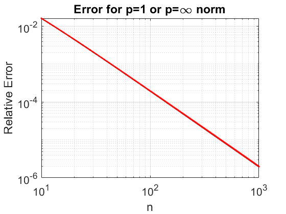
Table 1 shows the computed norms of the inverse and compares them with the estimate given by Theorem 3.3. For odd $n$ and $p\in\{1,\infty\}$ the norms are exact. For even $n$ , Theorem 3.3 gives an estimate that leads to a small gap. This gap relative to the estimate becomes negligible with an increase in $n$ . To support this statement, the reader is referred to Fig. 1 and Fig. 2 in log scales. The numerical tests are performed for all even $n$ from $10$ to $1000$ . The relative error is computed as $|\|A^{-1}\|_{p}-UBound|/\|A^{-1}\|_{p}$ , where $UBound=(n+1)^{2}\left((n+1)^{2}+8\right)/384$ from Theorem 3.3. As shown in Fig. 2 (left), the relative error decreases as $n$ increases for $p=1$ or $p=\infty$ . On the other hand, according to the numerical observation the difference between $\|A\|_{2}$ and the upper bound become constant relative to the norm as $n$ increases, see Fig. 2 (right).

Table 1: Computed

\|A^{-1}\|_{p}

and the estimates, for the clamped-clamped case.

$n$	$p=$			Upper bound from
	1	2	$\infty$	Theorem 3.3
49	16,328	12,527	16,328	16,328
50	17,658	13,558	17,658	17,672
99	260,625	199,939	260,625	260,625
100	271,150	208,055	271,150	271,203
150	1,354,225	1,038,976	1,354,225	1,354,343

Refer to caption — Figure 1: The upper bound and actual norm $p=1$ or $p=\infty$ (left) and $p=2$ (right) in log scale

For $n\geq 5$ , the factor $(1+8/(n+1)^{2})/384\leq 11/3474$ . So, alternatively, if $K$ satisfies the condition in the above theorem, we can have a simpler bound: $L_{p}<11/3474$ . This factor approaches $1/384$ from above as $n\to\infty$ . Since the latter is slightly less than the former, for a fixed $K$ , one can expect a slight improvement of convergence by increasing $n$ .

4 Numerical Results

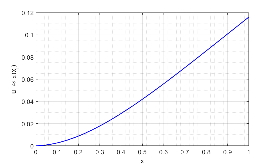
In this section, we present numerical results from solving (1) with (2) or (3) using the fixed point method(15). We compare the observed convergence with the theoretical bound given by (17) and Theorem 2.4 (for the clamped-free case) or Theorem 3.3 (for the clamped-clamped case).The fixed point method (15) is declared to have reached a convergence if $\|\bm{u}^{\ell+1}-\bm{u}^{\ell}\|_{p}<10^{-6}$ , where $p\in\{1,2,\infty\}$ . Solutions at convergence are shown in Figure 3 for the clamped-free and clamped-clamped case, with $K=1$ .

For both cases, the actual convergence rates are lower than the estimate (Tables 2–5), with increasing gaps between the two as $K$ increases. As $\|A^{-1}\|_{p}$ is exact, except for $p=2$ , (due to the explicit inverse of $A$ ), this suggests that the gap in the convergence rate is mainly due to the estimate $\|G\|_{p}<1$ . The numerical experiments suggest that the simple fixed-point method (15) can be used for a wider range of $K$ than suggested by the theoretical results. For instance, with $K=386$ and $n=99$ , we have $L_{p}=1.006$ . The method still however converges to the solution at the maximum rate of $0.5278$ .

Table 2: Observed maximum convergence rate for clamped-free case, with

n=50

. In brackets are the theoretical rate based on Theorem 2.4.

	$p=$
$K$	$1$		$2$		$\infty$
$1/8$	0.010	[0.016]	0.010	[0.016]	0.010	[0.017]
1	0.074	[0.125]	0.074	[0.125]	0.074	[0.125]
8	0.400	[1.000]	0.400	[1.000]	0.402	[1.000]

Table 3: Observed maximum convergence rate for clamped-free case, with

n=99

. In brackets are the theoretical rate based on Theorem 2.4.

	$p=$
$K$	$1$		$2$		$\infty$
$1/8$	0.010	[0.016]	0.010	[0.016]	0.010	[0.017]
1	0.074	[0.125]	0.074	[0.125]	0.074	[0.125]
8	0.400	[1.000]	0.400	[1.000]	0.402	[1.000]

Table 4: Observed maximum convergence rate for the clamped-clamped case, with

n=49

. In brackets are the theoretical rate based on Theorem 3.3.

	$p=$
$K$	$1$		$2$		$\infty$
$1/8$	0.0003	[0.0033]	0.0003	[0.00033]	0.0003	[0.00033]
1	0.0020	[0.0026]	0.0020	[0.0026]	0.0020	[0.0026]
8	0.0158	[0.0209]	0.0159	[0.0209]	0.0161	[0.0209]
32	0.0615	[0.0836]	0.0619	[0.0836]	0.0627	[0.0836]
128	0.2223	[0.3344]	0.2237	[0.3344]	0.2262	[0.3344]

Table 5: Observed maximum convergence rate for the clamped-clamped case, with

n=100

. In brackets are the theoretical rate based on Theorem 3.3

	$p=$
$K$	$1$		$2$		$\infty$
$1/8$	0.0002	[0.00033]	0.0002	[0.00033]	0.0003	[0.00033]
1	0.0020	[0.0026]	0.0020	[0.0026]	0.0020	[0.0026]
8	0.0157	[0.0208]	0.0159	[0.0208]	0.0160	[0.0208]
32	0.0614	[0.0834]	0.0618	[0.0834]	0.0625	[0.0834]
128	0.2218	[0.3336]	0.2232	[0.3336]	0.2257	[0.3336]

5 Conclusion

The explicit inverse formula for pentadiagonal matrices arising in the fourth-order nonlinear beam boundary value problem were constructed. The explicit formula helped computing some norms of their inverse, used to estimate the convergence of a fixed-point iteration for solving the nonlinear system of equations. Further research on the convergence upper bounds is necessary to extend our knowledge of the convergence rate in the fixed point method.

Acknowledgment

BK and YA wishes to acknowledge the research grant, No AP08052762, from the Ministry of Education and Science of the Republic of Kazakhstan and the Nazarbayev University Faculty Development Competitive Research Grant (NUFDCRG), Grant No 110119FD4502.

References

[1] Chaojie Wang, Hongyi Li, and Di Zhao. An explicit formula for the inverse of a pentadiagonal toeplitz matrix. Journal of Computational and Applied Mathematics, 278:12–18, 2015.
[2] EL Allgower. Exact inverses of certain band matrices. Numerische Mathematik, 21(4):279–284, 1973.
[3] Wayne W Barrett and Philip J Feinsilver. Inverses of banded matrices. Linear Algebra and its Applications, 41:111–130, 1981.
[4] Lars Rehnqvist. Inversion of certain symmetric band matrices. BIT Numerical Mathematics, 12(1):90–98, 1972.
[5] Murray Dow. Explicit inverses of toeplitz and associated matrices. ANZIAM Journal, 44:185–215, 2002.
[6] Wayne W Barrett. A theorem on inverse of tridiagonal matrices. Linear Algebra and Its Applications, 27:211–217, 1979.
[7] Jiteng Jia, Tomohiro Sogabe, and Moawwad El-Mikkawy. Inversion of k-tridiagonal matrices with toeplitz structure. Computers & Mathematics with Applications, 65(1):116–125, 2013.
[8] P Rózsa. On the inverse of band matrices. Integral equations and operator theory, 10(1):82–95, 1987.
[9] Xi-Le Zhao and Ting-Zhu Huang. On the inverse of a general pentadiagonal matrix. Applied Mathematics and Computation, 202(2):639–646, 2008.
[10] F Diele and L Lopez. The use of the factorization of five-diagonal matrices by tridiagonal toeplitz matrices. Applied mathematics letters, 11(3):61–69, 1998.
[11] Xiao-Guang Lv and Ting-Zhu Huang. A note on inversion of toeplitz matrices. Applied Mathematics Letters, 20(12):1189–1193, 2007.
[12] Bakytzhan Kurmanbek, Yogi Erlangga, and Yerlan Amanbek. Inverse properties of a class of seven-diagonal (near) toeplitz matrices. arXiv preprint arXiv:2103.09868, 2021.
[13] Mohamed Elouafi. Explicit inversion of band toeplitz matrices by discrete fourier transform. Linear and Multilinear Algebra, 66(9):1767–1782, 2018.
[14] Yerlan Amanbek, Zhibin Du, Yogi Erlangga, Carlos M. da Fonseca, Bakytzhan Kurmanbek, and António Pereira. Explicit determinantal formula for a class of banded matrices. Open Mathematics, 18(1):1227–1229, 2020.
[15] Bakytzhan Kurmanbek, Yerlan Amanbek, and Yogi Erlangga. A proof of andjelić-fonseca conjectures on the determinant of some toeplitz matrices and their generalization. Linear and Multilinear Algebra, pages 1–8, 2020.
[16] Yaroslav Shitov. The determinants of certain (0, 1) toeplitz matrices. Linear Algebra and its Applications, 2021.
[17] H Grob. Schwelldruck im belchentunnel. In Proc. Int. Symp. für Untertagebau, Luzern, pages 99–119, 1972.
[18] PA Von Wolffersdorff and S Fritzsche. Laboratory swell tests on overconsolidated clay and diagenetic solidified clay rocks. Proc. Geotechnical Measurements and Modelling, Karlsruhe, AA Balkema Pub, pages 407–412, 2003.
[19] Piotr Skrzypacz, Daulet Nurakhmetov, and Dongming Wei. Generalized stiffness and effective mass coefficients for power-law euler–bernoulli beams. Acta Mechanica Sinica, pages 1–16, 2019.
[20] Dongming Wei, Yu Liu, Dichuan Zhang, Match Wai Lun Ko, and Jong R Kim. Numerical analysis for retaining walls subjected to swelling pressure. In Proceedings of 2016 International Conference on Architecture, Structure and Civil Engineering (ICASCE’16), London (UK) Mar, pages 26–27, 2016.

	$\displaystyle\\|\bm{u}^{\ell}-\bm{u}^{\ell-1}\\|_{p}$	$\displaystyle=\\|h^{4}KA^{-1}(\exp(-\bm{u}^{\ell-1})-\exp(-\bm{u}^{\ell-2}))\\|_{p}$
		$\displaystyle=h^{4}K\\|A^{-1}\left(\exp(-\bm{u}^{\ell-2})+G(\bm{u}^{\ell-1}-\bm{u}^{\ell-2})-\exp(-\bm{u}^{\ell-2})\right)\\|_{p}$
		$\displaystyle=h^{4}K\\|A^{-1}G(\bm{u}^{\ell-1}-\bm{u}^{\ell-2})\\|_{p},$

$\displaystyle\sum_{j=1}^{n}\|m_{ij}\|$	$\displaystyle=$	$\displaystyle\sum_{j=1,j\neq 1}^{n}\|m_{ij}\|+\|m_{ii}\|=\sum_{j=1,j\neq 1}^{n}\|\widetilde{m}_{ij}\|+\|1+\widetilde{m}_{ii}\|$
	$\displaystyle\leq$	$\displaystyle 1+\|\widetilde{m}_{ii}\|+\sum_{j=1,j\neq i}^{n}\|\widetilde{m}_{ij}\|$
	$\displaystyle=$	$\displaystyle 1+\sum_{j=1}^{n}\|\widetilde{m}_{ij}\|.$