Invariant cones for linear elliptic systems
with gradient coupling

I. Capuzzo Dolcetta

{}^{\hbox{\small{ a}}}

, L. Rossi

{}^{\hbox{\small{ a,b }}}

and A. Vitolo

{}^{\hbox{\small{ c}}}

{}^{\hbox{a }}

Dipartimento di Matematica, Sapienza Università di Roma, Italy

{}^{\hbox{b }}

CAMS, CNRS-EHESS, Paris, France

{}^{\hbox{c }}

Dipartimento di Ingegneria Civile, Università di Salerno, Italy

Abstract. We discuss counterexamples to the validity of the weak Maximum Principle for linear elliptic systems with zero and first order couplings and prove, through a suitable reduction to a nonlinear scalar equation, a quite general result showing that some algebraic condition on the structure of gradient couplings and a cooperativity condition on the matrix of zero order couplings guarantee the existence of invariant cones in the sense of Weinberger [21].

MSC 2010 Numbers: 35J47, 35J70, 35B50, 35P30, 35D40 ¹¹1This work has been partially supported by GNAMPA-INdAM
[email protected]
[email protected]
[email protected]

Keywords and phrases: elliptic differential inequalities, weak Maximum Principle, invariant cones, Bellman operators, principal eigenvalue.

1 Introduction

We consider smooth vector-valued functions $u=(u_{1},\dots,u_{m})$ of the variable $x$ in a bounded open subset $\Omega\subset{\mathbb{R}}^{n}$ satisfying linear systems of partial differential inequalities of the following form

Au+\sum_{i=1}^{n}B^{(i)}D_{i}u+Cu\geq 0\;\;\hbox{in}\;\;\Omega

(1.1)

where $A$ is the second order operator

Au=\left(\begin{array}[]{c}\Delta u_{1}\\ .\\ .\\ .\\ \Delta u_{m}\end{array}\right)

(1.2)

$B^{(i)}$ and $C$ are $m\times m$ real matrices and with constant coefficients, and for $i=1,\dots,n$ ,

D_{i}u=\left(\begin{array}[]{c}\frac{\partial u_{1}}{\partial x_{i}}\\ .\\ .\\ .\\ \frac{\partial u_{m}}{\partial x_{i}}\end{array}\right)

(1.3)

denotes the $i-th$ column of the Jacobian matrix of the vector function $u$ .
Note that the above defined structure of the systems allows coupling between the $u_{j}$ and their gradients but not at the level of second derivatives.
Specific assumptions on the $B^{(i)}$ and $C$ will be made later on.

Systems of this kind naturally arise in several different contexts such as modeling of simultaneous diffusions of $m$ substances which decay spontaneously or in the case of systems describing switching diffusion processes in probability theory. In the latter case the homogeneous Dirichlet problem for system (1.1) describes discounted exit times from $\Omega$ , see for example [11].

We are interested here in investigating the validity of the weak Maximum Principle, wMP in short, that is the sign propagation property from the boundary to the interior for solutions $u=(u_{1},\dots,u_{m})$ of the differential inequalities (1.1), i.e.,

\mathbf{wMP}:\quad u\leq 0\ \mbox{on}\ \partial\Omega\ \ \implies\ \ u\leq 0\ \mbox{in}\ \Omega.

(1.4)

The vector function $u$ will be always assumed to belong to $[C^{2}(\Omega)]^{m}\cap[C^{0}(\overline{\Omega})]^{m}$ and we will adopt the standard notation $u\leq 0$ if $u_{j}\leq 0$ for each $j=1,\dots,m$ . We adopt the same notation for real-valued matrices, namely for a matrix $A$ , $A\geq 0$ means that all its entries are nonnegative.
The validity of wMP is well-understood in the scalar case $m=1$ even for general degenerate elliptic fully nonlinear partial differential inequalities such as

F(x,u,\nabla u,\nabla^{2}u)\geq 0

in a bounded $\Omega$ and also in some unbounded domain of ${\mathbb{R}}^{n}$ , see [8, 9] for recent results in this direction. Let us point out that the wMP property in the scalar case is related, and in fact equivalent, to the positivity of the principal eigenvalue (may be a pseudo one, if degeneracy occur in the dependence of $F$ with respect to Hessian matrix $\nabla^{2}u$ ) of the Dirichlet problem for $F$ , see [2],[3].

The case $m>1$ has been the object of several papers mainly in the case of diagonal weakly coupled systems, that is when the matrices $B^{(i)}$ are diagonal and couplings between the functions $u_{j}$ only occur at the level of zero-order terms, described by a matrix $C=(c_{jk})_{j,k}$ , satisfying the cooperativity condition

c_{jk}\geq 0\ \ \mbox{for }j\neq k\;,\qquad\sum_{k=1}^{m}c_{jk}\leq 0\ \ \mbox{for }\,j=1,\dots,m

(1.5)

Referring to the aforementioned exit time model, condition (1.5) requires the discount factor for the $j$ -th process to dominate the sum of the interactions coefficients with all the other processes.

In the framework of purely weak cooperative couplings, let us mention the results in Section 8 of the book by Protter and Weinberger [18] and the references therein. For generalizations of those results in some semilinear cases see [19],[5],[1], while [6] contains results in the same direction concerning fully nonlinear uniformly elliptic operators $F=F(x,u,\nabla u,\nabla^{2}u)$ .
The recent paper [10] extends the validity of some of the results in [6] concerning wMP to a large class of fully nonlinear degenerate elliptic operators.
In particular, for the case of linear systems as (1.1) with no coupling in first derivatives (i.e. when each $B^{(i)}$ is diagonal), the main result in [10] is that wMP holds true for system (1.1) provided $C$ is cooperative.
Let us also point out that the main result in [10] holds even in the more general case where the Laplace operator is replaced by more general expressions $\mathrm{Tr}(A^{j}\nabla^{2}u_{j})$ satisfying $\mathrm{Tr}(A^{j})>0$ for $j=1,\dots,m$ .

When coupling in first order terms occurs in (1.1), simple examples as the following one taken from [6] show that the wMP property (1.4) may indeed fail:

Example 1.

The vector $u(x_{1},x_{2})=(1-x_{1}^{2}-x_{2}^{2},\frac{1}{3}x_{1}^{3}+4x_{2}-20)$ is a solution of

\begin{cases}\displaystyle\Delta u_{1}+\frac{\partial u_{2}}{\partial x_{2}}=0\\ \displaystyle\Delta u_{2}+\frac{\partial u_{1}}{\partial x_{1}}=0\par\end{cases}

in the unit ball $\Omega\subset{\mathbb{R}}^{2}$ , $u_{1}=0$ , $u_{2}<0$ on $\partial\Omega$ but $u_{1}>0$ in $\Omega$ . Observe that the zero-order matrix is $C\equiv 0$ in this example, so that (1.5) is fulfilled.

As a matter of fact, even a first-order coupling of arbitrarily small size in the system can be responsible of the loss of wMP, as the following example shows:

Example 2.

The system

\begin{cases}\displaystyle\Delta u-\varepsilon\frac{\partial v}{\partial x_{1}}\geq 0\\ \displaystyle\Delta v-\varepsilon^{\prime}\frac{\partial u}{\partial x_{1}}\geq 0\end{cases}

in a bounded domain $\Omega\subset{\mathbb{R}}^{n}$ , fulfills wMP if and only if $\varepsilon=\varepsilon^{\prime}=0$ .
Indeed the validity of wMP when $\varepsilon=\varepsilon^{\prime}=0$ is classical. Conversely, if, say, $\varepsilon^{\prime}\neq 0$ , then wMP is violated by the pair

u(x)=\delta-|x-\bar{x}|^{2},\qquad v(x)=v(x_{1})=C(e^{-x_{1}}-H),

where $\bar{x}\in\Omega$ and $\delta>0$ is small enough to have $u<0$ on $\partial\Omega$ , and $C\gg 1$ , $H\gg 1$ .

Example 2 enlightens an instability property of wMP for cooperative systems with respect to first order perturbations. This is in striking contrast with the scalar case. Indeed, for a uniformly elliptic scalar inequality, not only the presence of a first order term does not affect the validity of wMP when the zero-order term is nonpositive, but in addition wMP is stable with respect to perturbations of the coefficients, in the $L^{\infty}$ norm. This can be seen as a consequence of the fact that wMP is characterized by the positivity of the associated principal eigenvalue, and the latter depends continuously on the coefficients of the operator, see e.g. [18, 3] and also [5, 6] where such characterization in terms of the same notion of principal eigenvalue as in [3] is extended to cooperative systems without first-order coupling. Example 2 reveals either that such notion does not exist when there is a first-order coupling, or that it is not continuous with respect to the coefficients.

According to the above considerations, two perspectives can be adopted in order to investigate the sign-propagation properties for coupled systems such as (1.1). The first one consists in strengthening the hypotheses on the coefficients of the operators, namely the cooperativity condition (1.5). The second one is to replace wMP by some different kind of propagation property which reflects in some way the geometry of the coupling terms. We will explore both directions.

Observe that the systems in Examples 1 and 2 fulfill the cooperativity condition (1.5) in the “border case”, that is, when all inequalities are replaced by equalities. A natural question is then whether it is possible, for the wMP to hold, to allow some coupling in first-order terms in the system, at least when the cooperativity conditions (1.5) hold with strict inequalities, i.e.,

c_{jk}\geq K\ \ \mbox{for }j\neq k\;,\qquad\sum_{k=1}^{m}c_{jk}\leq-K\ \ \mbox{for }\,j=1,\dots,m,

(1.6)

with $K$ possibly very large. The next result shows that this is not possible.

Proposition 1.

Let $\varepsilon>0$ , $\alpha,\tilde{c}\geq 0$ . Then the following system with $m=2$ and $n=1$

\left\{\begin{array}[]{lll}u^{\prime\prime}\pm\varepsilon v^{\prime}-cu+\alpha v\geq 0\\ v^{\prime\prime}-\tilde{c}v\geq 0\quad\quad\quad\quad\quad\quad x\in I_{\rho}=(0,\rho)\end{array}\right.

(1.7)

where $u$ , $v$ are scalar functions of $x\in{\mathbb{R}}$ does not satisfy wMP, provided that

\zeta(\rho\sqrt{c})\sqrt{c}>\frac{\alpha}{\varepsilon}\quad\mbox{ where }\ \zeta(\tau):=\frac{\cosh\tau-1}{\sinh\tau-\tau}\;.

(1.8)

Remark 3.

Since $\zeta(0^{+})=+\infty$ and $\zeta(+\infty)=1$ , this proposition entails that, for every $\varepsilon,K>0$ , there exists a system of the type (1.1), with $B^{(i)}$ satisfying $|B^{(i)}_{jk}|\leq\varepsilon$ and $C=(c_{jk})_{j,k}$ satisfying (1.6), for which wMP fails. Namely, even an arbitrary small amount of coupling at the level of first derivatives can prevent the validity of wMP although the zero order matrix is, so to say, “very strongly cooperative”. It also shows that, for any $\varepsilon,c>0$ and $\alpha,\tilde{c}\geq 0$ , wMP fails for (1.7) in a small enough interval $I_{\rho}$ . The fact that wMP fails when the diagonal zero-order term $c$ is sufficiently large or when the size $\rho$ of the interval is sufficiently small can be surprising, if one has in mind the picture for the scalar equation (where both having a large –negative– zero-order term and a small domain help the validity of the maximum principle).
This phenomenon could be related to a non-monotonic structure of the system when a first-order coupling is in force.

Remark 4.

A few more comments are in order here. We are considering a system with coupled gradients ( $\varepsilon>0$ ). The first part of Proposition 1 says that wMP cannot be satisfied in all bounded domains as soon as $\varepsilon>0$ , whatever the amount of cooperativity ( $\alpha>0$ ) is. The second part means that in a fixed interval wMP fails for $c$ large enough. In cooperative systems under consideration ( $0\leq\alpha\leq c$ ) an excess of coercivity with respect to the coupling ( $c$ large compared with $\alpha/\varepsilon$ ) seems to be responsible for invalidating wMP. In particular this is the case in any interval $I_{\rho}$ when $\alpha=0$ .

We exhibit in Proposition 2 below that the same qualitative phenomenon occurs for a larger class of systems. The proofs of Propositions 1 and 2 are detailed in Section 2.

Proposition 2.

For every $\varepsilon\neq 0$ , $\tilde{c}>0$ and $\tilde{\varepsilon},\alpha,\beta\in{\mathbb{R}}$ , there exists $c>0$ large enough such that the system

\left\{\begin{array}[]{lll}u^{\prime\prime}-\varepsilon v^{\prime}-cu+\alpha v\geq 0\\ v^{\prime\prime}-\tilde{\varepsilon}u^{\prime}-\tilde{c}v+\beta u\geq 0\end{array}\right.\quad\text{in }(0,1)

(1.9)

violates the wMP.
If, instead, $c>0$ is also fixed in the system (1.9), there exists an interval $I\subset(0,1)$ in which such system does not fulfill the wMP.

Let us turn now to the positive results. The study of sufficient conditions for the validity of the weak Maximum Principle in the form wMP in the case where coupling occurs also at the level of first or second order derivatives is apparently less explored in literature, see however [13],[14],[15] and also [17],[16] for the related issue of maximum norm estimates of the form $\sup_{x\in\Omega}|u(x)|\leq C\,\sup_{x\in\Omega}|f(x)|$ for solutions $u$ of non-homogeneous systems of equations involving higher order couplings.

The wMP property (1.4) can be understood in the framework of the general theory of invariant sets introduced by H. F. Weinberger in [21] in the context of elliptic and parabolic weakly coupled systems. We refer to the recent paper by G. Kresin and V. Mazya [15] where the notion of invariance is thoroughly developed for general systems with couplings at the first and the second order in the case $C\equiv 0$ .
According to the notion introduced in [21], a set $S\subseteq{\mathbb{R}}^{m}$ is invariant for system (1.1) if the following property holds

\mathbf{INV}:\qquad u(x)\in S\;\;\hbox{for all}\;x\in\partial\Omega\ \ \implies\ \ u(x)\in S\;\;\hbox{for all}\;x\in\Omega

(1.10)

The sign propagation property (1.4) can then be rephrased as the property of the negative orthant ${\mathbb{R}}^{m}_{-}=\{u=(u_{1},\dots u_{m}):u_{j}\leq 0\,\,,\,j=1,\dots,m\}$ being an invariant set for system (1.1) of partial differential inequalities.
In [21] it is proved in particular that wMP holds for weakly coupled uniformly elliptic systems such as

\mathrm{Tr}(A^{j}\nabla^{2}u_{j})+b^{j}\cdot\nabla u_{j}+f(u)=0\;,\;j=1,\dots,m

(1.11)

under the condition that the vector field $f$ satisfies the property that for any $p$ belonging to the outward normal cone to ${\mathbb{R}}^{m}_{-}$ at a point $u$ on the boundary of ${\mathbb{R}}^{m}_{-}$ the inequality

p\cdot f(u)\leq 0

(1.12)

holds. For $f(u)=Cu$ , this geometric condition turns out to be the cooperativity property (1.5) of matrix $C$ . Note also that this condition implies that ${\mathbb{R}}^{m}_{-}$ is invariant under the flow $du/dt=Cu\,,t>0$ .

We recall that Proposition 1 entails that ${\mathbb{R}}^{m}_{-}$ may fail to be an invariant set even when the coupling of the first order terms is very small. As a matter of fact, the first order matrix of system (1.7) is

\left(\begin{array}[]{cc}0&-\varepsilon\\ 0&0\end{array}\right)

which is not diagonalizable. This is indeed consistent with results in [15]. It is in fact shown in that paper, see in particular results in Section 3, that the sufficient conditions involving the relations between the geometry of a closed convex set $S$ and the matrices $B^{(i)}$ which imply the invariance of $S$ , necessarily require, in the case $S={\mathbb{R}}^{m}_{-}$ , the diagonal structure of the first order couplings.

On the account of the example (1.7) exhibited in Proposition 1 we are forced to investigate the validity of a weaker form of the sign propagation property or, in other words, to single out an appropriate invariant set for system (1.1) when first order couplings occur.

It turns out that under some algebraic conditions, including notably the simultaneous diagonalizability of the matrices $B^{(i)}$ , a cone propagation type result holds:

Theorem 3.

Let $\Omega$ be a bounded open subset of ${\mathbb{R}}^{n}$ . Assume that there exists an invertible $m\times m$ matrix $Q$ such that, for all $i=1,\dots,n$ ,

Q^{-1}B^{(i)}Q=\mathrm{Diag}\big{(}\beta_{1}^{(i)},\dots,\beta_{m}^{(i)}\big{)}\quad\hbox{for some}\;\;\beta^{(i)}_{j}\in{\mathbb{R}},\ \ \ (j=1,\dots,m)

(1.13)

Q^{-1}\geq 0

(1.14)

and, moreover,

Q^{-1}CQ\ \ \hbox{fulfills the cooperativity condition \eqref{coop}}

(1.15)

Then the convex cone $S=\{u\in{\mathbb{R}}^{m}:Q^{-1}u\leq 0\}$ is invariant for system (1.1).

Remark 5.

Concerning the linear algebraic conditions of Theorem 3, observe first that a matrix $Q$ simultaneously satisfying (1.11) for $i=1,\dots,n$ exists if the $B^{(i)}$ ’s have a common basis of eigenvectors. This is the case when the matrices $B^{(i)}$ commute each other for all $i=1,\dots,n.$ Observe also that if $Q$ is an invertible M-matrix, that is $Q=sI-X$ where $X\geq 0$ and $s$ is strictly greater than the spectral radius of $X$ , then $Q$ fulfills condition (1.14), see [4].
Next, it is worth to point out that conditions (1.14) and (1.15) are compatible.
For example, $Q=\left(\begin{array}[]{cc}2&-1\\ -1&2\end{array}\right)$ is an invertible M-matrix, $C=\left(\begin{array}[]{cc}-3&2\\ 1&-2\end{array}\right)$ is cooperative and $Q^{-1}CQ=\left(\begin{array}[]{cc}-4&3\\ 0&-1\end{array}\right)$ is cooperative as well.
If no coupling occurs in first derivatives, so that $Q=Q^{-1}=I$ , the above result reproduces the one in [10].

Remark 6.

A related remark is that permutation matrices satisfies both $Q^{-1}\geq 0$ and $Q\geq 0$ , so that in this case the conclusion of Theorem 3 is in fact that the negative orthant $R^{m}_{-}$ is invariant. However, it is easy to check that in this situation condition (1.13) implies that each $B^{(i)}$ is diagonal and the results of [10] apply.
A further remark is that one cannot expect in general the invariance of the negative orthant $R^{m}_{-}$ . This is indeed coherent with results in [15]; Lemma 2 there states in fact that the geometric sufficient condition on the matrices $B^{(i)}$ guaranteeing the invariance of $R^{m}_{-}$ implies their diagonal structure.

Remark 7.

Theorem 3 can in fact be extended (with a completely analogous proof) to a second order matrix operator

Au=\left(\begin{array}[]{c}\mathrm{Tr}(A\nabla^{2}u_{1})\\ .\\ .\\ .\\ \mathrm{Tr}(A\nabla^{2}u_{m})\end{array}\right)

(1.16)

where $A$ is a positive semidefinite matrix such that $A\nu\cdot\nu\geq\lambda>0$ for some direction $\nu\in{\mathbb{R}}^{n}$ . For some applications of this notion of directional uniform ellipticity condition see [7],[8],[9],[20].

A key role in the proof of this result, which is postponed to the next section, is based on a reduction to a suitable fully nonlinear scalar differential inequality governed by the elliptic convex Bellman-type operator $F$ defined, on scalar functions $\psi:\Omega\to{\mathbb{R}}$ , as

F[\psi]=\Delta\psi+\max_{j=1,\dots,m}\sum_{i=1}^{n}\beta^{(i)}_{j}\frac{\partial\psi}{\partial x_{i}}=\Delta\psi+\max_{j=1,\dots,m}b^{j}\cdot\nabla\psi

(1.17)

where $\beta^{(i)}_{j}$ are as in (1.13) and $b^{j}:=(\beta^{(1)}_{j},\dots,\beta^{(m)}_{j})$ . The main ingredients in the proof are results in [10], see in particular Theorems 1.1 and 1.3, and the notion of generalized principal eigenvalue for scalar fully nonlinear degenerate elliptic operators and its relations with the validity of wMP, see [2].

The next example provides a simple illustration of the result of Theorem 3:

Example 8.

Let $u=(u_{1},u_{2})$ be a solution of

\begin{cases}\displaystyle\Delta u_{1}+6\frac{\partial u_{1}}{\partial x_{1}}+\frac{\partial u_{2}}{\partial x_{1}}-u_{1}\geq 0\\ \displaystyle\Delta u_{2}-8\frac{\partial u_{1}}{\partial x_{1}}-u_{2}\geq 0\end{cases}

in a bounded domain $\Omega\subset{\mathbb{R}}^{n}$ . In this case $B^{(1)}=\left(\begin{array}[]{cc}6&1\\ -8&0\end{array}\right)$ , $B^{(2)}=0$ , $C=\left(\begin{array}[]{cc}-1&0\\ 0&-1\end{array}\right)$ and Theorem 3 applies with

Q=\left(\begin{array}[]{cc}-1&1/2\\ 4&-1\end{array}\right)\quad Q^{-1}=\left(\begin{array}[]{cc}1&1/2\\ 4&1\end{array}\right)

yielding that inequality $u_{2}\leq\min(-2u_{1};-4u_{1})$ propagates from $\partial\Omega$ to the whole $\Omega$ .

The result of Theorem 3 can be somewhat refined by a suitable weakening of the assumptions there. Firstly, observe that $B^{(i)}$ is not necessarily diagonalizable. A suitable change of basis generally generally leads to an upper triangular matrix, which yields a real Jordan canonical form of $B^{(i)}$ .
Suppose that the $B^{(i)}$ ’s have a common eigenspace of dimension $k\leq m$ and consider a basis of $\mathbb{R}^{m}$ where the first $k$ vectors are linearly independent (common) eigenvectors of $B^{(i)}$ , then we can find an $m\times m$ invertible real matrix $\hat{Q}$ that produces a real Jordan canonical form $J^{(i)}=\hat{Q}^{-1}B^{(i)}\hat{Q}$ , where the $k\times m$ sub-matrix with the first $k$ rows is made up by a $k\times k$ diagonal block $\Lambda$ plus the $k\times(m-k)$ zero matrix.

In this setting we have the following:

Theorem 4.

Assume in addition to the above that the $k\times m$ sub-matrix containing the first $k$ rows of $\hat{C}=\hat{Q}^{-1}C\hat{Q}$ is made by a cooperative $k\times k$ block plus the $k\times(m-k)$ zero matrix. Let $p_{ij}$ be the entries of the matrix $\hat{P}:=\hat{Q}^{-1}$ .
If the $k\times m$ sub-matrix with the first $k$ rows of $\hat{P}$ is positive, then the closed convex set

\hat{S}=\left\{u\in{\mathbb{R}}^{m}:\sum_{j=1}^{m}p_{1j}u_{j}\leq 0,\dots,\sum_{j=1}^{m}p_{kj}u_{j}\leq 0\right\}

is invariant for the system (1.1).

An illustrative example is provided next:

Example 9.

Consider the $2\times 2$ system

\begin{cases}\displaystyle\Delta u_{1}+\frac{\partial u_{2}}{\partial x_{1}}-u_{1}\geq 0\\ \displaystyle\Delta u_{2}+\frac{\partial u_{1}}{\partial x_{1}}-u_{2}\geq 0\end{cases}

in a domain $\Omega$ of ${\mathbb{R}}^{2}$ . In this case $B^{(1)}=\left(\begin{array}[]{cc}0&1\\ 1&0\end{array}\right)$ , $B^{(2)}=0$ , $C=\left(\begin{array}[]{cc}-1&0\\ 0&-1\end{array}\right)$ and Theorem 4 applies with

\hat{Q}=\left(\begin{array}[]{cc}1&1\\ 1&-1\end{array}\right)\quad\hat{Q}^{-1}=\left(\begin{array}[]{cc}1/2&1/2\\ 1/2&-1/2\end{array}\right)

Since the first row of $\hat{P}=\hat{Q}^{-1}$ is nonnegative the above result yields the invariance of the convex set $S=\{u=(u^{1},u^{2}):u^{1}+u^{2}\leq 0\}$ .
Note that wMP, that is the invariance of ${\mathbb{R}}^{2}_{-}$ , does not hold true in this example. Indeed, the vector $u=\big{(}(x_{1}-x_{1}^{2})(x_{2}-x_{2}^{2})^{3},(x_{1}^{2}+2x_{1}-4)(x_{2}-x_{2}^{2})\big{)}$ is a solution in the square $\Omega=[0,1]\times[0,1]$ taking non positive values on $\partial\Omega$ with $u_{2}\leq 0$ , $u_{1}\geq 0$ in $\Omega$ .

2 Proofs of the results

The first part of this section is dedicated to the proofs of Proposition 1 and 2.

Proof of Proposition 1.

We restrict to the case $-\varepsilon$ , with $\varepsilon>0$ . In fact, we can reduce to it by using the change of coordinate $x\to\rho-x$ . We also observe that the argument is not affected by $\tilde{c}\geq 0$ , so that we will omit to mention it when discussing on the parameters.

Firstly, we observe that $v(x)=-x$ obviously satisfies the second equation with $v\leq 0$ in $[0,\rho]$ .
Next, we introduce the sequence of functions

u_{k}(x)=-\frac{\varepsilon}{c}\left\{\frac{1-e^{-\sqrt{c}/k}}{2\sinh(\sqrt{c}/k)}\,e^{\sqrt{c}x}+\frac{e^{\sqrt{c}/k}-1}{2\sinh(\sqrt{c}/k)}\,e^{-\sqrt{c}x}-1-\frac{\alpha}{\varepsilon}\left(\frac{\sinh(\sqrt{c}x)}{k\sinh(\sqrt{c}/k)}-x\right)\right\}.

(2.1)

Then, a direct computation, shows that for all $k\in\mathbb{N}$ ,

u_{k}^{\prime\prime}-\varepsilon v^{\prime}-cu_{k}+\alpha v=0\ \ \hbox{\rm in}\ I_{\rho}\equiv(0,\rho)

(2.2)

and $u_{k}(0)=0$ .

The case $c=0$ is ruled out either by taking the limit as $k\to+\infty$ or directly by putting $v=-x$ and $c=0$ in the above equation.

Note also that for $k\to\infty$

\begin{split}u_{k}(x)\to u_{0}(x)&=-\frac{\varepsilon}{c}\left\{\cosh\sqrt{c}x-1-\frac{\alpha}{\varepsilon}\left(\frac{\sinh\sqrt{c}x}{\sqrt{c}}-x\right)\right\}\end{split}

(2.3)

Let the parameters $\varepsilon$ , $c$ , $\alpha$ and $\rho$ be fixed. For large $k\in\mathbb{N}$ :

\begin{split}u_{k}^{\prime}(0)&=-\frac{\varepsilon}{c}\left\{\frac{1-\cosh(\sqrt{c}/k)}{\sinh(\sqrt{c}/k)/\sqrt{c}}-\frac{\alpha}{\varepsilon}\left(\frac{\sqrt{c}/k}{\sinh(\sqrt{c}/k)}-1\right)\right\}\\ &=\frac{\varepsilon}{2k}+o(1/k)\end{split}

(2.4)

so that $u^{\prime}_{k}(0)>0$ for $k$ large enough.

Since $u_{k}(0)=0$ , we also have $u_{k}(x)>0$ for some $x\in I_{\rho}$ for such $k\in\mathbb{N}$ . So wMP will be violated if $u_{k}(\rho)\leq 0$ .

Next, computing (2.3) for $x=\rho$ ,

\begin{split}u_{k}(\rho)&=-\frac{\varepsilon\sqrt{c}}{\sinh\sqrt{c}\rho-\sqrt{c}\rho}\left\{\cosh\sqrt{c}\rho-1-\frac{\alpha}{\varepsilon}\left(\frac{\sinh\sqrt{c}\rho}{\sqrt{c}}-\rho\right)\right\}+u_{k}(\rho)-u_{0}(\rho)\\ &=-\frac{\varepsilon\sqrt{c}}{\sinh\sqrt{c}\rho-\sqrt{c}\rho}\left\{\zeta(\sqrt{c}\rho)\sqrt{c}-\frac{\alpha}{\varepsilon}\right\}+u_{k}(\rho)-u_{0}(\rho)\end{split}

(2.5)

where

\begin{split}\zeta(\tau)&=\frac{\cosh\tau-1}{\sinh\tau-\tau}.\end{split}

(2.6)

Therefore condition $\zeta(\sqrt{c}\rho)\sqrt{c}>\frac{\alpha}{\varepsilon}$ , see (1.8), yields $u_{k}(\rho)\leq 0$ , for large $k\in\mathbb{N}$ , so that wMP is not satisfied. Once established this fact, we search for condition (1.8) to prove that wMP fails.
A straightforward calculation shows that $\zeta(\tau)\to\infty$ as $\tau\to 0^{+}$ and $\zeta(\tau)\to 1$ as $\tau\to\infty$ . Therefore there exists $\rho_{0}=\rho_{0}(c;\frac{\alpha}{\varepsilon})$ such that condition (1.8) holds for $\rho<\rho_{0}$ , and wMP is not satisfied, thereby proving that as soon as $\varepsilon>0$ there are intervals $I_{\rho}$ , small enough, where wMP fails, whatever $c$ and $\alpha$ are.

On the other hand, let $\rho>0$ be fixed. The function $\zeta(\sqrt{c}\rho)\sqrt{c}$ is increasing with respect to $c$ , and $\zeta(\sqrt{c}\rho)\to 1$ as $c\to\infty$ , so that

\lim_{c\to\infty}\zeta(\sqrt{c}\rho)\sqrt{c}=\infty.

(2.7)

Hence there exists $c_{0}=c_{0}(\rho;\frac{\alpha}{\varepsilon})$ such that condition (1.8) holds for $c>c_{0}$ , and wMP is not satisfied, thereby proving that as soon as $\varepsilon>0$ then wMP fails in any interval $I_{\rho}$ and for any $\alpha\geq 0$ when a sufficiently large $c$ is taken.

By the increasing monotonicity of the function $c\to\zeta(\sqrt{c}\rho)\sqrt{c}$ we get

\inf_{c>0}\zeta(\sqrt{c}\rho)\sqrt{c}=\lim_{c\to 0^{+}}\zeta(\sqrt{c}\rho)\sqrt{c}=\frac{3}{\rho}\,.

It follows that, if $\frac{\alpha}{\varepsilon}<\frac{3}{\rho}$ , then condition (1.8) is satisfied for all $c>0$ . This means that in this case we can choose $c_{0}(\rho;\frac{\alpha}{\varepsilon})=0$ .

Finally, recalling that $\zeta(\sqrt{c}\rho)\to 1$ as $c\to\infty$ , then $\zeta(\sqrt{c}\rho)\sqrt{c}\cong\sqrt{c}$ for $c\geq c_{1}(\rho)$ . Hence condition (1.8) is equivalent to

\sqrt{c}>\frac{\alpha}{\varepsilon}.

(2.8)

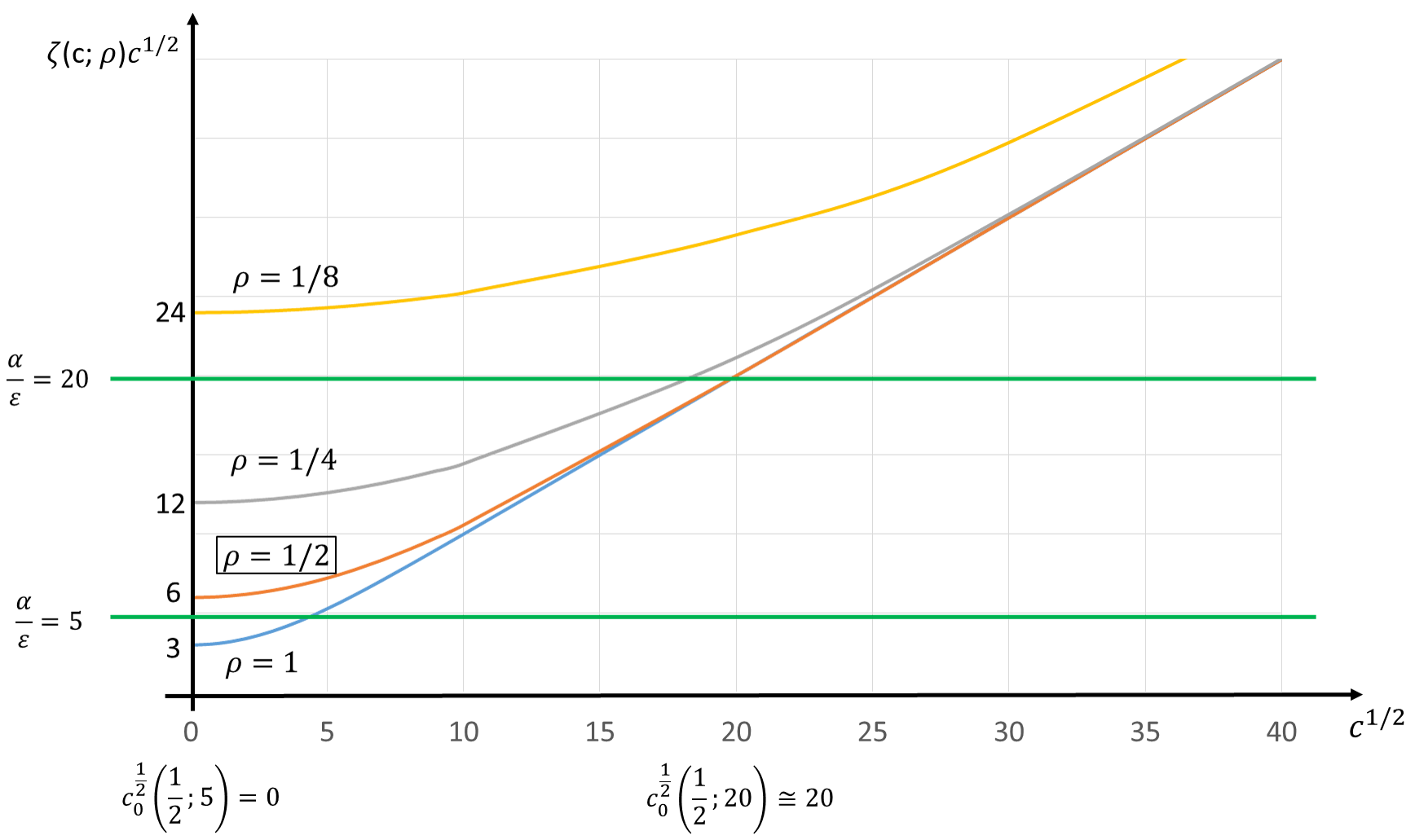
It follows that, if $\frac{\alpha}{\varepsilon}>c_{1}$ , then we can choose $c_{0}(\rho;\frac{\alpha}{\varepsilon})=\left(\frac{\alpha}{\varepsilon}\right)^{2}$ . ∎

Refer to caption — Figure 1: The function $\zeta(\sqrt{c}\rho)\sqrt{c}$

A picture of the function $c\to\zeta(\sqrt{c}\rho)\sqrt{c}$ for different values of $\rho>0$ is shown in Figure 1, where condition (1.8) with the threshold $c_{0}$ is graphically exhibited on the track $\rho=\frac{1}{2}$ for different values of $\frac{\alpha}{\varepsilon}$ .

Proof of Proposition 2.

Up to replacing $u(x),v(x)$ with $u(-x),v(-x)$ , it is not restrictive to assume that $\varepsilon>0$ . We claim that, for $c$ sufficiently large, there exists a pair $(u,v)$ satisfying (1.9) in a strict sense, namely

\left\{\begin{array}[]{lll}\inf_{(0,1)}\Big{(}u^{\prime\prime}-\varepsilon v^{\prime}-cu+\alpha v\Big{)}>0\\ \inf_{(0,1)}\Big{(}v^{\prime\prime}-\tilde{\varepsilon}u^{\prime}-\tilde{c}v+\beta u\Big{)}>0\end{array}\right.

such that $u(0)=0>u(1)$ , $v(0)\leq 0$ , $v(1)\leq 0$ and $u^{\prime}(0)=0$ . Then, for $\delta>0$ sufficiently small, the pair of functions $(u(x)+\delta x,v(x))$ still satisfies the system (1.9) and both functions are $\leq 0$ on the boundary of $(0,1)$ , but $u(x)>0$ for $x>0$ small, hence the wMP is violated.

Let us construct the pair of strict subsolutions $(u,v)$ . They are defined as follows:

v(x)=x^{2}-x,\qquad u(x)=\sigma\chi(x),

where $\chi$ is a smooth, non-increasing function satisfying

\chi(0)=\chi^{\prime}(0)=0,\qquad\chi(x)=-1\ \ \text{for }\,x\geq\min\Big{\{}\,\frac{1}{4}\,,\,\frac{\varepsilon}{4|\alpha|+1}\,\Big{\}}

and $\sigma$ is a positive constant that will be chosen later. We compute, for $x\in(0,1)$ ,

v^{\prime\prime}-\tilde{\varepsilon}u^{\prime}-\tilde{c}v+\beta u\geq 2-\sigma\big{(}|\beta|+\tilde{\varepsilon}\|\chi^{\prime}\|_{L^{\infty}((0,1))}\big{)},

which is larger than $1$ for $\sigma\leq\sigma_{1}:=1/(|\beta|+\tilde{\varepsilon}\|\chi^{\prime}\|_{L^{\infty}((0,1))}+1)$ . Next, for $x\in(0,1)$ , we have that

\displaystyle u^{\prime\prime}-\varepsilon v^{\prime}-cu+\alpha v

\displaystyle\geq\varepsilon(1-2x)-|\alpha|x-\sigma|\chi^{\prime\prime}|-c\sigma\chi.

We estimate the right-hand considering first $0<x\leq\min\{1/4,\varepsilon/(4|\alpha|+1)\}$ , where we have

u^{\prime\prime}-\varepsilon v^{\prime}-cu+\alpha v\geq\frac{\varepsilon}{4}-\sigma\|\chi^{\prime\prime}\|_{L^{\infty}((0,1))},

which is larger than $\varepsilon/8$ for $\sigma\leq\sigma_{2}:=\varepsilon/(8\|\chi^{\prime\prime}\|_{L^{\infty}((0,1))})$ . While, for $\min(1/4,|\varepsilon|/(4|\alpha|+1))\!<\!x\!<\!1$ , we see that

u^{\prime\prime}-\varepsilon v^{\prime}-cu+\alpha v\geq-\varepsilon-|\alpha|+c\sigma,

which is positive for $c>(\varepsilon+|\alpha|)/\sigma$ . Summing up, taking $\sigma=\min\{\sigma_{1},\sigma_{2}\}$ and then $c>(\varepsilon+|\alpha|)/\sigma$ , we have that $(u,v)$ satisfies (1.9) in a strict sense. The first statement of the proposition is thereby proved.

Let us turn to the second statement. We have seen above that wMP fails for (1.9) provided $c$ is larger than some $\bar{c}>0$ , and more precisely that it is violated by a pair $(u,v)$ with $v<0$ on $(0,1)$ and $u>0$ somewhere. Consider the pair $(u,v)$ associated with $c=\bar{c}$ and let $I$ be a connected component of the set where $u>0$ in $(0,1)$ , hence $u=0$ on $\partial I$ . For $c\leq\bar{c}$ there holds in $I$ ,

u^{\prime\prime}-\varepsilon v^{\prime}-cu+\alpha v\geq u^{\prime\prime}-\varepsilon v^{\prime}-\bar{c}u+\alpha v\geq 0.

This means that the wMP fails in $I$ and then concludes the proof. ∎

Let us go now to the proof of Theorem 3.

Proof of Theorem 3.

Assume that $u\in[C^{2}(\Omega)]^{m}\cap[C^{0}(\overline{\Omega})]^{m}$ satisfies (1.1) and that $u\leq 0$ on $\partial\Omega$ . Set

\hat{B}^{(i)}:=Q^{-1}B^{(i)}Q\ \ \ \text{and}\ \ \ \hat{C}:=Q^{-1}CQ.

Observe that the change of unknown $u=Qv$ gives, on the account of assumptions (1.13), (1.14), that $v$ satisfies

Av+\sum_{i=1}^{n}\hat{B}^{(i)}D_{i}v+\hat{C}v\geq 0\;\;\hbox{in}\;\;\Omega\;\;\hbox{and}\;\;v\leq 0\;\hbox{on}\;\;\partial\Omega

(2.9)

that is, componentwise,

\left\{\begin{array}[]{lll}\Delta v_{1}+b^{1}\cdot\nabla v_{1}+\hat{C}_{1}v\,\,\,\;\,\,\geq 0\\ \qquad\qquad\cdots\\ \Delta v_{m}+b^{m}\cdot\nabla v_{m}+\hat{C}_{m}v\geq 0\\ \end{array}\right.

(2.10)

where $b^{j}=(\beta^{(1)}_{j},\dots,\beta^{(m)}_{j})$ and $\hat{C}_{j}$ is the $j$ -th row of $\hat{C}$ , for $j=1,\dots,m$ .
We now employ the argument of the proof of Theorem 1 in [10] which reduces the above system to a scalar inequality governed by the uniformly elliptic (nonlinear) Bellman operator $F$ in (1.17). By viscosity calculus results based on the cooperativity condition (1.15), see [10, 6], since $v=(v_{1},\dots,v_{m})$ is a classical solution of (2.9) then the scalar function

v^{*}(x):=\max_{j=1,\dots,m}(v_{j})^{+}(x)\,,

where “⁺” denotes the positive part, is a continuous weak solution in the viscosity sense, see [12], of

F[v^{*}]\geq 0\;\;\hbox{in}\;\;\Omega\;\;\hbox{and}\;\;v^{*}=0\;\hbox{on}\;\;\partial\Omega\,.

(2.11)

Suppose indeed that a smooth function $\varphi$ touches from above $v^{*}$ at some point in $\Omega$ . If at that point $v^{*}=0$ then clearly $F[\varphi]\geq 0$ there. Otherwise $\varphi$ touches from above the component $v_{j}$ realizing the positive maximum $v^{*}$ at that point and thus there holds

\Delta\varphi+b^{j}\cdot\nabla\varphi+\hat{C}_{j}v\geq 0.

But then recalling that $\hat{C}_{j}$ fulfills the cooperativity condition (1.5), one infers that

\hat{C}_{j}v\leq v_{j}\sum_{k}\hat{C}_{jk}\leq 0,

whence again $F[\varphi]\geq 0$ .

In order to apply the general result of [2] we need to show that the generalized principal eigenvalue, see [2], of $F$ is positive, which amounts to finding a strict supersolution which is strictly positive in $\overline{\Omega}$ . The latter is simply provided by $\psi(x)=\psi(x_{1},\dots,x_{m})=1-\delta e^{\gamma x_{1}}$ . Indeed, this function satisfies

F[\psi]=-\delta\gamma e^{\gamma x_{1}}\Big{(}\gamma+\min_{j=1,\dots,m}\beta_{j}^{(1)}\Big{)},

which is strictly negative in ${\mathbb{R}}^{n}$ provided $\gamma>|\min_{j=1,\dots,m}\beta_{j}^{(1)}|$ . We then choose $\delta$ small enough, depending on $\gamma$ and $\Omega$ , so that $\psi>0$ in $\overline{\Omega}$ . Summing up, $\psi$ is positive in $\overline{\Omega}$ and satisfies there $F[\psi]<0$ , hence also $F[\psi]+\lambda\psi<0$ for $\lambda>0$ suitably small. This implies that the numerical index $\mu_{1}(F,\Omega)$ defined by

\mu_{1}(F,\Omega)=\sup\{\lambda\in{\mathbb{R}}:\psi\in C(\overline{\Omega}),\ \psi>0,\ F[\psi]+\lambda\psi\leq 0\;\mbox{in}\;\Omega\}

(2.12)

is strictly positive. Therefore, according to [2], the weak Maximum Principle for the scalar problem (2.11) holds, that is $v^{*}\leq 0$ in $\Omega$ .

This means that $Q^{-1}u=v\leq 0$ in $\Omega$ and the proof is complete. ∎

We conclude the section with the proof of Theorem 4

Proof of Theorem 4.

Following the same lines of the proof of Theorem 3, we set $u=\hat{Q}v$ . When multiplying by $\hat{P}=\hat{Q}^{-1}$ , this time we keep, by assumption, the positivity for the first $k$ equations, which again by the assupmtions made are decoupled in the gradient variables. So, letting $\tilde{C}$ be the diagonal part of $\hat{C}$ and $\tilde{v}=(v_{1},\dots,v_{k})$ , we get

\left\{\begin{array}[]{lll}\Delta v_{1}+b^{1}\cdot\nabla v_{k}+\tilde{C}_{1}\tilde{v}\geq 0\\ \qquad\qquad\cdots\\ \Delta v_{k}+b^{m}\cdot\nabla v_{k}+\tilde{C}_{k}\tilde{v}\geq 0\\ \end{array}\right.

(2.13)

where $\tilde{C}_{j}$ is the $j$ -th row of $\hat{C}$ . The conclusion follows as in the proof of Theorem 2 with $k$ instead of $m$ . ∎

References

[1] H. Amann, Maximum principles and principal eigenvalues. (English summary) Ten mathematical essays on approximation in analysis and topology. 1–60, Elsevier B.V., Amsterdam, 2005. E.F. Beckenbach, R. Bellman, Inequalities. Springer-Verlag (1961).
[2] H. Berestycki, I. Capuzzo Dolcetta, A. Porretta, L. Rossi, Maximum Principle and generalized principal eigenvalue for degenerate elliptic operators. J. Math. Pures Appl. (9) 103 (2015), 1276–1293.
[3] H. Berestycki, L. Nirenberg, S.N. Varadhan, The principal eigenvalue and maximum principle for second-order elliptic operators in general domains. Comm. Pure Appl. Math. 47 (1994), no. 1, 47–92.
[4] A. Berman, R.J. Plemmons, Nonnegative Matrices in the Mathematical Sciences. Classics in Applied Mathematics, SIAM, Philadelfia (1994).
[5] I. Birindelli, E. Mitidieri, G. Sweers, Existence of the principal eigenfunction for cooperative elliptic systems in a general domain. Differential Equations 35 (3) (1999).
[6] J. Busca, B. Sirakov, Harnack type estimates for nonlinear elliptic systems and applications, Ann. I. H. Poincaré 21 (2004) 543–590.
[7] L. A. Caffarelli, Y.Y. Li and L. Nirenberg, Some remarks on singular solutions of nonlinear elliptic equations III: viscosity solutions including parabolic operators. Comm. Pure Appl. Math. 66 (2013), no. 1, 109–143.
[8] I. Capuzzo Dolcetta, A. Vitolo, The weak maximum principle for degenerate elliptic operators in unbounded domains. Int. Math. Res. Not. IMRN 2018, no. 2, 412–431.
[9] I. Capuzzo Dolcetta, A. Vitolo, Directional ellipticity on special domains: weak maximum and Phragmén-Lindelöf principles. Nonlinear Anal. 184 (2019), 69–82.
[10] I. Capuzzo Dolcetta, A. Vitolo, Weak Maximum Principle for Cooperative Systems: the Degenerate Elliptic Case, Journal of Convex Analysis Volume 28 (2021), No. 2
[11] Z. Q. Chen, Z. Zhao, Potential theory for elliptic systems, The Annals of Probability 1996, Vol. 24, No. 1, 293-319
[12] M.G. Crandall, H. Ishii, P.L. Lions, User’s guide to viscosity solutions of second order partial differential equations. Bull. Am. Math. Soc., New Ser. 27 (1992), pp. 1–67.
[13] G.I. Kresin and V.G. Maz’ya, On the maximum principle with respect to smooth norms for linear strongly coupled parabolic systems, Functional Differential Equations, 5:3-4 (1998), 349–376.
[14] G. Kresin and V. Maz’ya, Maximum Principles and Sharp Constants for Solutions of Elliptic and Parabolic Systems, Math. Surveys and Monographs, 183, Amer. Math. Soc., Providence, Rhode Island, 2012.
[15] G. Kresin, V. Maz’ya, Invariant convex bodies for strongly elliptic systems, J. Anal. Math. 135 (2018), no. 1, 203–224.
[16] Xu Liu, Xu Zhang, The weak maximum principle for a class of strongly coupled elliptic differential systems. Journal of Functional Analysis 263 (2012) 1862–1886.
[17] M. Miranda, Sul teorema del massimo modulo per una classe di sistemi ellittici di equazioni del secondo ordine e per le equazioni a coefficienti complessi. Istituto Lombardo (Rend.Sc.) A 104 736-745 (1970).
[18] M.H. Protter, H.F. Weinberger. Maximum Principles in Differential Equations. Springer-Verlag, New York, (1984).
[19] G. Sweers, Strong positivity in $C(\overline{\Omega})$ for elliptic systems. Math. Z. 209 (1992) 251–271.
[20] A. Vitolo, Singular elliptic equations with directional diffusion, Math.Eng. 3 (2021) no. 3 pp.1–16.
[21] H.F. Weinberger, Invariant sets for weakly coupled parabolic and elliptic systems. Rendiconti di Matematica 1 (1975), Vol. 8, Serie VI.

Invariant cones for linear elliptic systems with gradient coupling