Interrelated Thermalization and Quantum Criticality in a Lattice Gauge Simulator
Abstract
Gauge theory and thermalization are both foundations of physics and nowadays are both topics of essential importance for modern quantum science and technology Wiese:2013uq ; Tagliacozzo:2013oa ; Zohar:2015qs ; Dalmonte:2016lg ; Banuls:2020sl ; Banuls:2020ro ; Aidelsburger:2022ca ; Nandkishore:2015mb ; Bloch2019 ; Ueda:2020qe . Simulating lattice gauge theories (LGTs) realized recently with ultracold atoms provides a unique opportunity for carrying out a correlated study of gauge theory and thermalization in the same setting Yang:2020oo ; Zhou:2021td . Theoretical studies have shown that an Ising quantum phase transition exists in this implemented LGT Sachdev:2002mi ; Fendley:2004cd ; Rico:2014tn ; Surace:2020lg ; Yao:2022qm , and quantum thermalization can also signal this phase transition Yao:2022qm . Nevertheless, it remains an experimental challenge to accurately determine the critical point and controllably explore the thermalization dynamics in the quantum critical regime due to the lack of techniques for locally manipulating and detecting matter and gauge fields. Here, we report an experimental investigation of the quantum criticality in the LGT from both equilibrium and non-equilibrium thermalization perspectives by equipping the single-site addressing and atom-number-resolved detection into our LGT simulator. We accurately determine the quantum critical point agreed with the predicted value Sachdev:2002mi ; Fendley:2004cd ; Rico:2014tn . We prepare a state deterministically and study its thermalization dynamics across the critical point, leading to the observation that this state thermalizes only in the critical regime Yao:2022qm . This result manifests the interplay between quantum many-body scars, quantum criticality, and symmetry breaking.
Since quantum gauge theories are computationally intractable in the non-perturbative regime, the idea of formulating gauge theories on discretized space-time lattices led to LGTs, and the developments of LGTs enable numerical simulation of gauge theories with various classical algorithms in the past decades Rothe:Book . Recently, a new trend is realizing LGTs in quantum simulators with ultracold atoms or trapped ions Martinez:2016rt ; Kokail:2019sv ; Schweizer:2019fa ; Mil:2020as ; Yang:2020oo ; Zhou:2021td . By taking the quantum advantage, these quantum simulation platforms offer the promise of a better understanding of LGTs than classical simulations.
One potential advantage of quantum simulation for studying LGTs lies in the non-equilibrium dynamics, such as quantum thermalization. In ultracold atom systems, the essential parameters in the gauge theory are tunable, allowing accessing different phases and the quantum criticality in between. Quantum criticality refers to a qualitative change of the ground state and the universal behavior of low-energy physics. On the contrary, thermalization dynamics usually involves highly excited states. Remarkably, it has been recently proposed that the thermalization dynamics of the state can also signal the quantum critical regime in the U(1) LGT Yao:2022qm . However, it is challenging to study these physics due to the lack of techniques for manipulating and detecting local matter and gauge fields in the previous experiments.
In this work, we report on an experimental study of both equilibrium and thermalization dynamics in the quantum critical regime of the U(1) LGT. We integrate the techniques of single-site manipulation of matter and gauge fields and atom-number-resolved detection into an updated LGT simulator. With these technical advances, we can monitor the local Gauss’s law and then perform the post-selection, which eliminates the processes violating local gauge symmetries. We can measure the order parameter with various system sizes to perform a proper finite-size scaling, which overcomes the finite-size effects and determines the critical point accurately. We can also deterministically prepare the state by addressing single atoms in a programmed manner. Equipped with these capabilities, we observe the nontrivial thermalization dynamics across the quantum critical regime Yao:2022qm .
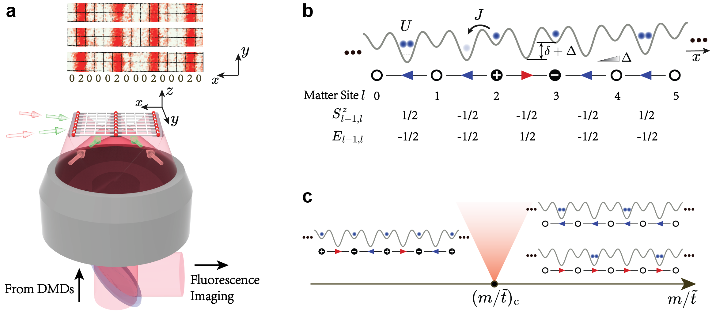
Our experimental system is shown in Fig. 1(a), which realizes a U(1) LGT using bosons in optical lattices, and the protocol is the same as that reported in the previous work Yang:2020oo . We combine a short lattice and a long lattice with twice the lattice spacing to create a one-dimensional superlattice, as shown in Fig. 1(b) Zhang:2022fb . When the deep lattice sites are doubly occupied, the on-site energy is , where is the on-site interaction energy and is the energy offset between deep and shallow lattices. When , the on-site energy of a doubly occupied site is nearly degenerate with an empty site, but is off-resonant with a singly occupied state. Thus, we only retain the empty and the doubly occupied states, and they are denoted by and , respectively. These deep lattice sites are viewed as gauge sites, and the shallow lattice sites are viewed as matter sites. This realizes the LGT written as Yang:2020oo
| (1) |
where labels the matter sites, and are bosonic operators for the matter fields. Spin- operators are defined in the deep lattices. Here is the mass of the matter field. is generated by a second-order hopping process because the long-range direct hoppings are suppressed by applying a tilting potential.
This model possesses local gauge symmetries because the Hamiltonian Eq. (1) is invariant under the local gauge transformation , and Yang:2020oo . This local gauge symmetry gives rise to a set of local conserved quantities . By introducing the electric field and the physical charge , the conservation can be written as
| (2) |
which is exactly the Gauss’s law of U(1) LGTs Yang:2020oo . A configuration of the electric field and Gauss’s law is also schematically shown in Fig. 1(b).
When focusing on the gauge sector with all , there are two phases in the Hamiltonian Eq. (1) as tuning . This can be easily seen by looking at two limits with . When , the matter field favors and therefore , leading to an antiferromagnetic state or at gauge sites. This leads to two-fold degenerate ground state. When , the matter field favors and therefore . This state does not break the original lattice translational symmetry. Hence the transition is a symmetry breaking transition of the Ising type, and detailed theoretical calculations predict the critical point at Sachdev:2002mi ; Fendley:2004cd ; Rico:2014tn . Signatures of two different phases have also been observed in the previous experiment Yang:2020oo .
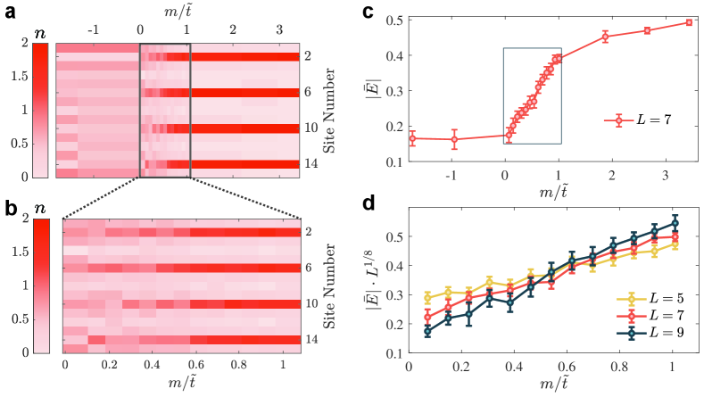
To accurately determine the quantum critical point, we first prepare a state with high fidelity utilizing the ability of single-site addressing (see Methods) at Hz, Hz, and Hz, corresponding to Weitenberg:2011ss . This state is an antiferromagnetic state in the gauge sites and empty sites in the matter sites. Here we prepare copies of identical chains along the direction, as shown in Fig. 1(a) [See also Fig. S1(f) in Methods]. Each chain contains gauge sites and matter sites, with a total of atoms in each chain ( as shown below). Then, we adiabatically ramp to the targeted critical regime around Hz, with a constant ramping speed Hz/. Such change of leaves and nearly unaffected, and it changes the value of to the critical regime, as shown in Fig. 2. Finally, the system is suddenly frozen and the atom number at each site is read out with the single-site-resolved microscope. Note that usually the fluorescence imaging cannot distinguish two atoms from zero atom at the same site Bakr:2009aq ; Sherson:2010sa . Here, before detection, we split two atoms into two sites of a double well along the direction if there are two atoms at the same site. This allows us to resolve atom number two from zero at a single site (see Methods). To mitigate the undesired effects from processes beyond the LGT, we post-select our data based on two rules: (i) the total atom number remains the same as that of the initial state, and (ii) the Gauss’s law Eq. (2) has to be obeyed for all sites. With the adiabatic ramping and the post-selection, we ensure that the ground state of the LGT at the targeted is reached. The results of single-site-resolved measurement of atom number distribution is shown in Fig. 2(a) for a range of .
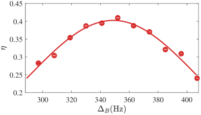
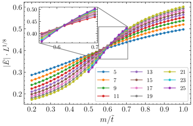
To locate the critical point, we measure the order parameter . This order parameter is the staggered magnetization, and given the definition of the electric field, this order parameter is also the spatial averaged electric field strength, denoted by . We plot as a function of with in Fig. 2(c), which exhibits a rapid change when is in the range . To more accurately determine the critical point, we zoom in this range and perform a finite-size scaling. We plot for different system size , and for the two-dimensional Ising universality class, the order parameter critical exponent and the correlation length critical exponent Francesco:Book . The crossing point of these curves locates the critical point (see Methods for numerical simulation). Here we indeed observe the crossing of three curves. However, since each data point has an error bar, it is not clear to visualize the exact crossing point. Hence, we consider each point as a normalized Gaussian distribution where , and are respectively the value and the error bar of each data point. We calculate the averaged Kullback–Leibler (KL) divergence of the three Gaussian distributions at each , which quantifies the degree of overlap between three Gaussian distributions. The averaged KL divergence is defined as Sgarro:1981id
| (3) |
We plot the as a function of in Fig. 4(a), and fitting the data yields a peak position at . This value is consistent with theoretical predictions Sachdev:2002mi ; Fendley:2004cd ; Rico:2014tn . Given the energy scale of our , the deviation from the theoretical critical value is less than Hz.
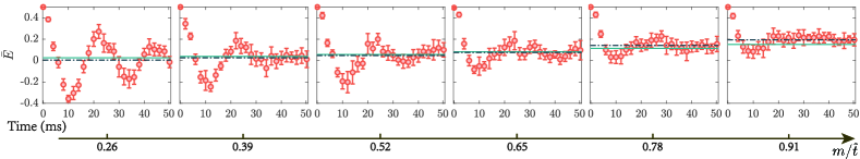
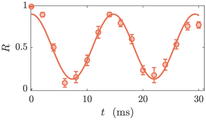
We then consider the quench dynamics. The same state is prepared as the initial state. Now, instead of adiabatic ramping, we suddenly change the value of to the targeted value nearby the critical point, with a typical time scale of . Here we fix Hz and Hz. The value of is larger than what we used for the adiabatic ramping process. This is because we find that even a weak spatial inhomogeneity can cause noticeable variations of from site to site, which can affect the time dynamics. A larger helps to reduce this variation in terms of and can significantly suppress the effects of the inhomogeneity. We record the spatial atom number distribution at different times during the real-time dynamics using a single-site-resolved microscope. We also apply the same post-selection to ensure that the dynamics is governed by the LGT. The measurements of time dynamics are shown in Fig. 3 for different values of .
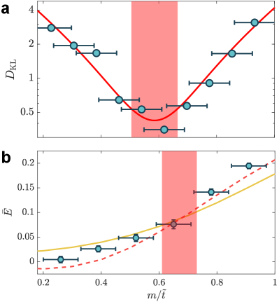
We fit the experimental data in Fig. 3 with a damped sinusoidal function , where , , , and are all fitting parameters. We obtain as the long-time steady value, as illustrated by the dashed lines in Fig. 3. Meanwhile, we can also theoretically extract the thermalization values , provided that the system obeys the eigenstate thermalization hypothesis and the initial state thermalizes Deutsch:1991qs ; Srednicki:1994ca ; Rigol:2008ta ; DAlessio:2016fq . is obtained by calculating . Here is an equilibrium density matrix of the LGT system, with the temperature determined by matching energy (see Methods). Previous work has predicted that for the PXP model, matches and the initial state thermalizes only in the quantum critical regime Yao:2022qm . These two values depart from each other away from the critical point . When , the ground state is two-fold degenerate and the state has large overlap with the ground state, and the ground state is always not thermalized. When , especially around , it is known that the PXP model hosts a set of many-body scar states as the system’s eigenstates Bernien:2017pm ; Turner:2018we ; Turner:2018qs . The state also has large overlap with the scar states, preventing it from thermalization Bernien:2017pm ; Turner:2018we ; Turner:2018qs . The PXP model is equivalent to this LGT model under the local gauge constraints of for all , and therefore, the discussion also applies to this LGT model Surace:2020lg ; ChengTA . In Fig. 4(b), we compare with , and our measurements agree with the prediction that only in the quantum critical regime Yao:2022qm .
In summary, we have performed a single-site-resolved quantitative experimental study of the quantum criticality in the U(1) LGT realized with bosons in optical lattices. Our study combines both the equilibrium property and the thermalization dynamics. Our system size is up to lattice sites, and our quantitative results agree well with the numerical results of exact diagonalization. This agreement benchmarks the validity of our ultracold atom quantum simulator quantitatively, and demonstrates this simulator as a powerful platform to study non-equilibrium dynamics of the gauge theory. In the near future, when our system size is enlarged several times, it will be beyond the capability of exact diagonalization. The experimental control and detection capability developed in this work can be used to study other interesting dynamical phenomena in this system, such as string breaking Banerjee:2012aq ; Hebenstreit:2013rt , dynamical transition between quantum phases Huang:2019dq ; Zache:2019dt , the false vacuum decay, and the confinement-deconfinement transition Surace:2020lg ; ChengTA ; Hauke . The current scheme of implementing the LGT can also be extended to higher dimensions Ott:2021sc .
Acknowledgement We thank Meng-Da Li, Qian Xie, Bo Xiao, Hui Sun, Wan Lin, An Luo for their help on building the experimental setup. This work was supported by NNSFC grant 12125409, Innovation Program for Quantum Science and Technology 2021ZD0302000.
References
- (1) Wiese, U.-J. Ultracold quantum gases and lattice systems: quantum simulation of lattice gauge theories. Annalen Der Physik 525, 777–796 (2013).
- (2) Tagliacozzo, L., Celi, A., Zamora, A. & Lewenstein, M. Optical Abelian lattice gauge theories. Ann. Phys. 330, 160–191 (2013).
- (3) Zohar, E., Cirac, J. I. & Reznik, B. Quantum simulations of lattice gauge theories using ultracold atoms in optical lattices. Rep. Prog. Phys. 79, 014401 (2015).
- (4) Dalmonte, M. & Montangero, S. Lattice gauge theory simulations in the quantum information era. Contemp. Phys. 57, 388–412 (2016).
- (5) Bañuls, M. C. et al. Simulating lattice gauge theories within quantum technologies. Eur. Phys. J. D 74, 1–42 (2020).
- (6) Bañuls, M. C. & Cichy, K. Review on novel methods for lattice gauge theories. Rep. Prog. Phys. 83, 024401 (2020).
- (7) Aidelsburger, M. et al. Cold atoms meet lattice gauge theory. Phil. Trans. R. Soc. A. 380, 20210064 (2022).
- (8) Nandkishore, R. M. & Huse, D. A. Many-Body Localization and Thermalization in Quantum Statistical Mechanics. Annu. Rev. Condens. Matter Phys. 6, 15–38 (2015).
- (9) Abanin, D. A., Altman, E., Bloch, I. & Serbyn, M. Colloquium: Many-body localization, thermalization, and entanglement. Rev. Mod. Phys. 91, 021001 (2019).
- (10) Ueda, M. Quantum equilibration, thermalization and prethermalization in ultracold atoms. Nat Rev Phys 2, 669–681 (2020).
- (11) Yang, B. et al. Observation of gauge invariance in a 71-site Bose–Hubbard quantum simulator. Nature 587, 392–396 (2020).
- (12) Zhou, Z.-Y. et al. Thermalization dynamics of a gauge theory on a quantum simulator. Science 377, 311–314 (2022).
- (13) Sachdev, S., Sengupta, K. & Girvin, S. M. Mott insulators in strong electric fields. Phys. Rev. B 66, 075128 (2002).
- (14) Fendley, P., Sengupta, K. & Sachdev, S. Competing density-wave orders in a one-dimensional hard-boson model. Phys. Rev. B 69, 075106 (2004).
- (15) Rico, E., Pichler, T., Dalmonte, M., Zoller, P. & Montangero, S. Tensor Networks for Lattice Gauge Theories and Atomic Quantum Simulation. Phys. Rev. Lett. 112, 201601 (2014).
- (16) Surace, F. M. et al. Lattice Gauge Theories and String Dynamics in Rydberg Atom Quantum Simulators. Phys. Rev. X 10, 021041 (2020).
- (17) Yao, Z., Pan, L., Liu, S. & Zhai, H. Quantum many-body scars and quantum criticality. Phys. Rev. B 105, 125123 (2022).
- (18) Rothe, H. J. Lattice Gauge Theories. (World Scientific, 2012).
- (19) Martinez, E. A. et al. Real-time dynamics of lattice gauge theories with a few-qubit quantum computer. Nature 534, 516–519 (2016).
- (20) Kokail, C. et al. Self-verifying variational quantum simulation of lattice models. Nature 569, 355–360 (2019).
- (21) Schweizer, C. et al. Floquet approach to lattice gauge theories with ultracold atoms in optical lattices. Nat. Phys. 15, 1168–1173 (2019).
- (22) Mil, A. et al. A scalable realization of local U(1) gauge invariance in cold atomic mixtures. Science 367, 1128–1130 (2020).
- (23) Zhang, W.-Y. et al. Functional building blocks for scalable multipartite entanglement in optical lattices. arXiv preprint arXiv:2210.02936 (2022).
- (24) Weitenberg, C. et al. Single-spin addressing in an atomic Mott insulator. Nature 471, 319–324 (2011).
- (25) Bakr, W. S., Gillen, J. I., Peng, A., Fölling, S. & Greiner, M. A quantum gas microscope for detecting single atoms in a Hubbard-regime optical lattice. Nature 462, 74–77 (2009).
- (26) Sherson, J. F. et al. Single-atom-resolved fluorescence imaging of an atomic Mott insulator. Nature 467, 68–72 (2010).
- (27) Francesco, P. D., Mathieu, P. & Sénéchal, D. Conformal Field Theory. (Springer, 2012).
- (28) Sgarro, A. Informational divergence and the dissimilarity of probability distributions. CALCOLO 18, 293–302 (1981).
- (29) Deutsch, J. M. Quantum statistical mechanics in a closed system. Phys. Rev. A 43, 2046–2049 (1991).
- (30) Srednicki, M. Chaos and quantum thermalization. Phys. Rev. E 50, 888–901 (1994).
- (31) Rigol, M., Dunjko, V. & Olshanii, M. Thermalization and its mechanism for generic isolated quantum systems. Nature 452, 854–858 (2008).
- (32) D’Alessio, L., Kafri, Y., Polkovnikov, A. & Rigol, M. From quantum chaos and eigenstate thermalization to statistical mechanics and thermodynamics. Advances in Physics 65, 239–362 (2016).
- (33) Bernien, H. et al. Probing many-body dynamics on a 51-atom quantum simulator. Nature 551, 579–584 (2017).
- (34) Turner, C. J., Michailidis, A. A., Abanin, D. A., Serbyn, M. & Papić, Z. Weak ergodicity breaking from quantum many-body scars. Nat. Phys. 14, 745–749 (2018).
- (35) Turner, C. J., Michailidis, A. A., Abanin, D. A., Serbyn, M. & Papić, Z. Quantum scarred eigenstates in a Rydberg atom chain: Entanglement, breakdown of thermalization, and stability to perturbations. Phys. Rev. B 98, 155134 (2018).
- (36) Cheng, Y., Liu, S., Zheng, W., Zhang, P. & Zhai, H. Tunable Confinement-Deconfinement Transition in an Ultracold Atom Quantum Simulator. arXiv preprint arXiv:2204.06586 (2022).
- (37) Banerjee, D. et al. Atomic Quantum Simulation of Dynamical Gauge Fields Coupled to Fermionic Matter: From String Breaking to Evolution after a Quench. Phys. Rev. Lett. 109, 175302 (2012).
- (38) Hebenstreit, F., Berges, J. & Gelfand, D. Real-Time Dynamics of String Breaking. Phys. Rev. Lett. 111, 201601 (2013).
- (39) Huang, Y.-P., Banerjee, D. & Heyl, M. Dynamical Quantum Phase Transitions in U(1) Quantum Link Models. Phys. Rev. Lett. 122, 250401 (2019).
- (40) Zache, T. V. et al. Dynamical Topological Transitions in the Massive Schwinger Model with a Term. Phys. Rev. Lett. 122, 050403 (2019).
- (41) Halimeh, J. C., McCulloch, I. P., Yang, B. & Hauke, P. Tuning the Topological -Angle in Cold-Atom Quantum Simulators of Gauge Theories. arXiv preprint arXiv:2204.06570 (2022).
- (42) Ott, R., Zache, T. V., Jendrzejewski, F. & Berges, J. Scalable Cold-Atom Quantum Simulator for Two-Dimensional QED. Phys. Rev. Lett. 127, 130504 (2021).
- (43) Xiao, B. et al. Generating two-dimensional quantum gases with high stability. Chinese Physics B 29, 076701 (2020).
- (44) Yang, B. et al. Cooling and entangling ultracold atoms in optical lattices. Science 369, 550–553 (2020).
- (45) Yang, B. et al. Spin-dependent optical superlattice. Phys. Rev. A 96, 011602 (2017).
- (46) Cardy, J. L. Finite-size Scaling. (North-Holland, 1988).
- (47) Binder, K. & Heermann, D. W. Monte Carlo Simulation in Statistical Physics: An Introduction. (Springer, 2019).
METHODS AND SUPPLEMENTARY MATERIALS
I Experimental Procedure
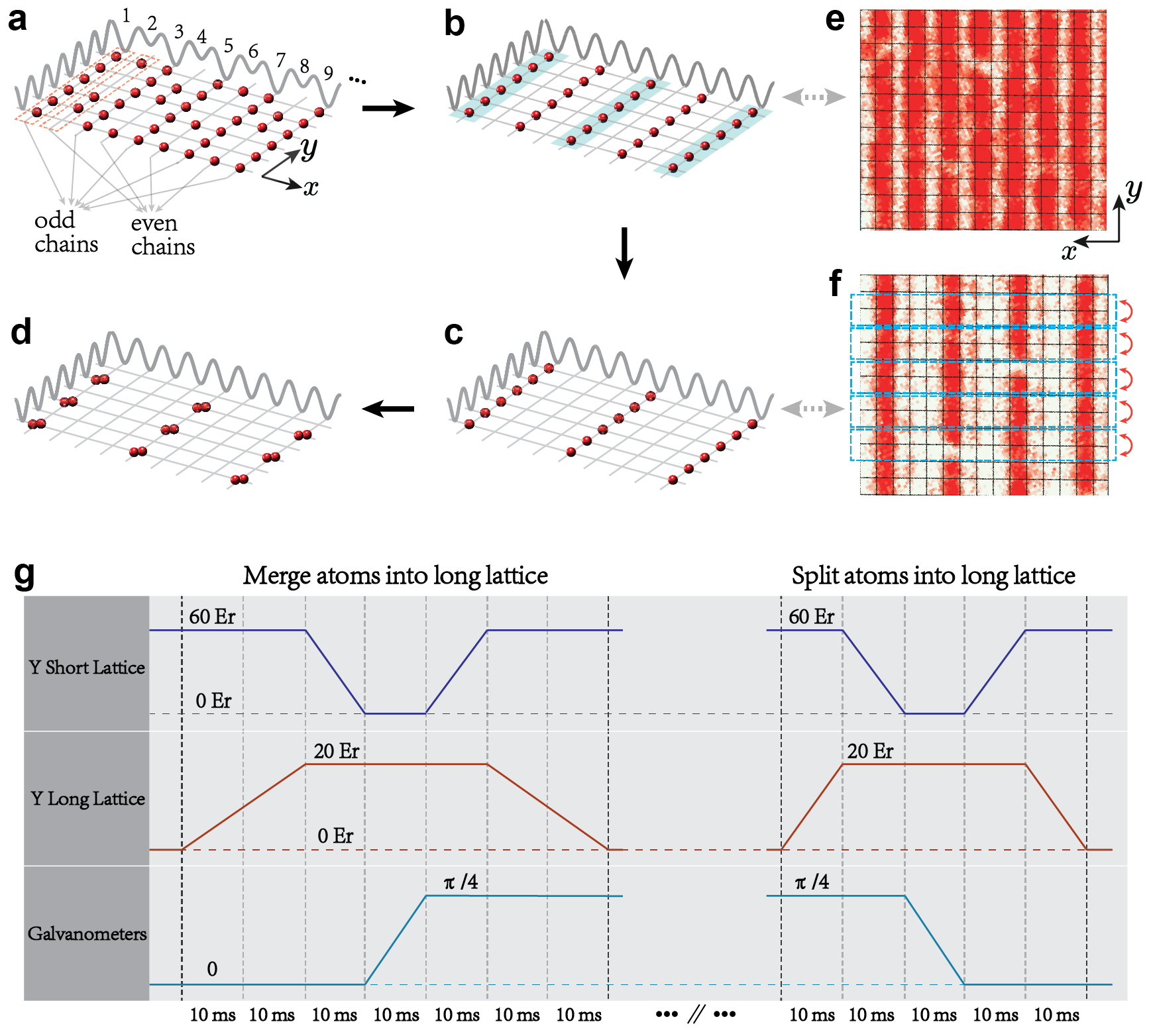
Initial state preparation. Our experiment begins by preparing a two-dimensional (2D) Bose-Einstein condensate of 87Rb atoms in the state, which has been described in our previous work Xiao:2020gt ; Zhang:2022fb . We then employ the recently demonstrated staggered-immersion cooling method to prepare a near-unity filling Mott insulator state Yang:2020ca ; Zhang:2022fb . As a result, we obtain a series of one-dimensional (1D) Mott insulators with a filling factor of prepared in the “odd chains” along the direction, as schematically shown in Fig. S1(a). Then, we remove the atoms in the “even chains” via site-dependent addressing Yang:2017sd , leaving a system with 1D Mott insulators only in the “odd chains”, as shown in Fig. S1(b). The next step is addressing the Mott-insulator chains in an alternating fashion, using a beam of wavelength reflected from a DMD Weitenberg:2011ss . For example, only the blue shaded chains in S1(b) are addressed. After that, we remove the unaddressed chains to prepares a series of Mott-insulator chains separated by , as shown in Fig. S1(c). The last step is to turn on the superlattice potential (not shown in Fig. S1) in the direction to merge every two atoms into one site Yang:2020ca . We end up with copies of initial state along the direction, as shown in Fig. S1(d). In terms of gauge field degrees of freedom, this state reads .
Atom number detection. To obtain the single-site-resolved atom occupancy of the final state, we split the atoms at each site into a double well along the direction using the time sequence shown in Fig. S1(g). Assuming that there are at most two atoms at the same site, this splitting process has three possible outcomes: (i) ; (ii) (); and (iii) . Finally, we perform a fluorescence imaging to record the atom parity distribution that can be used to reconstruct the atom number distribution before the splitting process Zhang:2022fb .
II Calibrations
Calibration of Hubbard parameters. The lattice depths of the “short lattice” and the “long lattice” along the and directions are calibrated using lattice modulation spectroscopy, the details can be found in our previous work Zhang:2022fb . The Hubbard parameters, tunneling strength and on-site interaction strength , are also calibrated with the same method described in our previous work Zhang:2022fb .
Calibration of staggered potential . In the experiment, the staggered potential is controlled by the depth of the “long lattice” along the direction. To calibrate , we start with the initial state shown in Fig. S1(c). Then, we ramp up the “long lattice” along the direction with to create the same staggered structure as that in Fig. 1(b). Next, a magnetic field gradient is applied to create an energy bias between two adjacent lattice sites along the direction. After that, we ramp down the “short lattice” along the direction from to in while keeping the “short lattice” along the direction at and let the system evolve for . Finally, we record the positions of the atoms using single-site-resolved fluorescence imaging. We measure the population fraction of the atoms that tunnel to its adjacent site as a function of the energy bias , as shown in Fig. S2. Since , this function should be peaked at , where the atoms undergo nearly resonant Rabi oscillation between adjacent sites. By fitting the data with a Gaussian function, we can extract the corresponding staggered potential . From the calibrated staggered potential and the interaction strength , we can determine the mass using .
Calibration of . To calibrate the pair hopping strength , we prepare multiple isolated systems of three sites with two atoms, and we start with the initial state . Then we quench the parameters and of the system to the targeted values while keeping . After evolving the system for a time , we post-select two states and . Let and denote the number of occurrences that we detect and respectively. We then plot the population fraction in Fig. S3 as a function of the evolution time. The pair hopping strength can be read out from the oscillation frequency of fitted by a sinusoidal function.
Adiabatic condition. To determine the adiabatic condition of the ramping process, we prepare the initial state and ramp from Hz [] to Hz [] with different ramping speeds. Then we plot the of the final state as a function of the ramping time. As one can see from Fig. S4, when the ramping time is longer than , the observable of the final state barely changes with the ramping time. This shows that the adiabatic condition is satisfied in this regime. In the experiment, we ramp from Hz to Hz in at a speed of Hz/ to fulfill the adiabatic condition.
III Numerical Simulation
Finite-size scaling. According to the theory of finite-size scaling (FSS) Cardy:Book_FSS ; Binder:Book , the absolute value of the order parameter scales with system size as
| (S1) |
Here, where the average is the quantum average over the ground state. is the order parameter critical exponent, is the correlation length critical exponent. is the reduced “temperature” with being the control parameter and being the critical point, and is the scaling function. Therefore, the critical point can be determined as the crossing point of different curves of plotted against .
Gauss’s law, in the gauge sector , means that the matter field configuration is completely determined by that of gauge sites. Therefore, the U(1) LGT (1) can be written in terms of the gauge fields only,
| (S2) |
where and are the standard Pauli operators. In the following, we shall employ this gauge field only Hamiltonian to perform exact diagonalization study under the open boundary condition to calculate . And this Hamiltonian is precisely the PXP model with an additional external field. The resulting finite-size scaling plot of the scaling variable is shown in Fig. S5.
Due to corrections to scaling, different curves will not cross at the single critical point. We fit the curves in the inset of Fig. S5 and then calculate the crossing point between the curve of system size and the curve of system size , which yields . Extrapolating to infinite size determines the critical point. In this way, our estimate of the critical point is , as shown in Fig. S6. Besides the order parameter, variables such as (here ), and the Binder cumulant can also be used for FSS analysis Binder:Book . Following the same procedure described above, the estimated critical point is using and using for FFS analysis. Taking into these slightly different values of into account, our estimated critical point is thus , in agreement with the more accurate estimate of Rico:2014tn . In summary, our numerical simulation demonstrates the applicability of measuring with different system sizes to accurately determine the critical point.

Computation of the thermalization values and the steady values. For a quantum system after a quench, a physical observable is expected to fluctuate around a steady value after the relaxation time . On the other hand, its thermal value is defined to be micro-canonical ensemble average of at the energy of the initial state. Due to the equivalence of statistical ensembles, the thermal value can also be calculated using the canonical ensemble at some temperature
| (S3) |
The temperature is determined by equating the ensemble averaged energy with the energy of the initial state
| (S4) |
where is the initial state. As explained in the previous section, we can employ the gauge fields only Hamiltonian Eq. (S2) to perform the calculation. We choose the staggered magnetization, i.e. , the spatial averaged electric field strength , as our observable , and proceed to use exact diagonalization to calculate its thermal value according to Eqs. (S3) and (S4). The result is shown as the solid yellow line in Fig. 4(b).
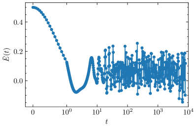
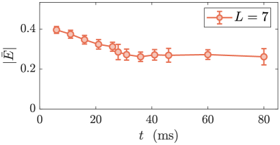
We then move to determine the relaxation time and the steady value. To this end, starting from the state, we evolve the system for a long time. A typical case for and is shown in Fig. S7. From this plot, we infer that the relaxation time of is less than (we use dimensionless time in unit of ) for this parameter setting. Repeating this process for other values of from to , we obtain a safe estimate of the upper bound of the relaxation time of as . By definition, the steady value can be evaluated as follows
| (S5) |
where is the wave function at time . In numerical calculation, we choose and average over around random sampled time evolution data points in time range to extract . We also increase the value of several times in doing the above average to confirm convergence. We plot thus obtained steady values as the red dashed line in Fig. 4(b).