Internal waves in 2D domains with ergodic classical dynamics
Abstract.
We study a model of internal waves in an effectively 2D aquarium under periodic forcing. In the case when the underlying classical dynamics has sufficiently irrational rotation number, we prove that the energy of the internal waves remains bounded. This involves studying the spectrum of a related 0-th order pseudodifferential operator at spectral parameters corresponding to such dynamics. For the special cases of rectangular and elliptic domains, we give an explicit spectral description of that operator.
1. Introduction
Below the surface layers of the ocean, the density field can be be approximated by a stable-stratified field. This means that the density depends only on depth and increases slowly with it. A standard model for internal waves is given by considering linear perturbations of such stable-stratified fluids, and is a central topic in oceanography. These perturbations occur naturally and can arise mechanically or thermodynamically. For a more complete introduction to the physics behind internal waves, see Mass [Maa05] and Sibgatullin–Ermanyuk [SE19].
In this paper, we consider an open, bounded, and simply-connected domain with a smooth boundary. Internal waves are modeled by the equation
| (1.1) |
with and . This is the Poincaré equation [Poi85], also called the Sobolev equation [Sob54]. This problem comes from the study of internal waves in a 2D aquarium with a constant Brunt-Vaïsälä frequency which we take equal to . The solution represents the stream function of the fluid velocity, meaning the velocity field is given by
| (1.2) |
Then (1.1) can be interpreted as the evolution of the stream function under periodic forcing in the interior of the domain with forcing profile . The Dirichlet boundary condition is simply saying that velocity of the fluid near the boundary must be tangent to the boundary, i.e. no forcing from the boundary. Let , and let and . Then the boundary forced equation
can be easily reduced to (1.1) by replacing with .


Rewriting (1.2) so that (1.1) reads like an evolution problem, we define
| (1.3) |
where denotes the Dirichlet Laplacian. Then satisfies the equation
| (1.4) |
The operator is bounded and self-adjoint, see [Ral73]. The solution can then be written using the functional calculus:
| (1.5) |
We are interested in its long-time behavior which equivalent to the long time behavior of the solution to (1.1). As the functional solution (1.5) becomes singular when the spectral parameter is equal to . Therefore studying the long-time behavior is closely related top the spectral properties of at .
Our main result concerns the behavior of when the underlying classical dynamics is ergodic. The relevant dynamics at forcing frequency is given by the chess billiard map, which is a -dependent family of circle diffeomorphism (see (2.4) for details and §2.1 for motivation). To every , we may assign a rotation number , which measures the average rotation of , see (2.5) for the precise definition. When the rotation number is irrational, the map is ergodic, which is the setting we will focus on.
Finally, we need a natural geometric assumption on the domain , called -simplicity [DWZ21], see Definition 2.1. For now, we emphasize that all strictly convex domains satisfy this assumption for all .
Theorem 1.
Let be open, bounded, and simply connected. Assume that is such that is -simple.
-
(a)
If the rotation number is irrational, then is not in the pure point spectrum of , i.e. is injective.
- (b)
-
(c)
If the rotation number is Diophantine, the spectral measure of satisfies, for all ,
Parts (b) and (c) of Theorem 1 were first proved by the second named author [Li23] (Theorem 2 and Theorem 1 respectively). This was done by studying a boundary reduced 0-th order pseudo-differential operator on the circle, found in [DWZ21]. The assumptions in (a) are weaker than the corresponding assumption of [Li23, Lemma 6.1], which assumes the eigenfunction to be smooth. It was already proven in [Arn61, Theorem 10], see also [Joh41].
In this paper, we give a simpler proof by directly constructing an inverse to a related eigenvalue problem (see (2.1)). We also describe the spectrum in two simple cases: rectangular and elliptic domains; the latter is related to the recent work of the first named author and Vidal [CdVV23] which studied the case rotating fluids in ellipsoids.
The spectral measure of can be numerically approximated using the methods developed in [Col21, CHT21, Col22]. Theorem 1 still holds for the square even though the boundary is not smooth. In that case, the rotation number can be computed as an explicit smooth function of , and so the spectral bound can be seen numerically in Figure 2.
Two examples where we can explicitly compute the spectrum of are given by and , the unit disk. For the square, the eigenfunctions are simply the Fourier modes. For the circle, we will give an explicit complete basis of consisting of solutions to the eigenvalue problem (2.1), see (4.11) and Figure 1. Then by changing the coordinates, we have spectral information about elliptic and rectangular domains.

Theorem 2.
If is an ellipse or if is a rectangle with sides parallel to the coordinate axis, the spectrum of is pure point dense in and the eigenvalues are exactly the values of for which the rotation number is rational.
For the theorem above, we emphasize that the ellipses we consider can be any nondegenerate linear transformation of a circle. This includes tilted ellipses with major and minor axis not necessarily parallel to the coordinate axis. On the other hand, the theorem fails for tilted rectangle; it is shown in [Ral73] that the spectrum contains an absolutely continuous part.
1.1. Related works
Analysis of (1.1) goes back to [Sob54]. The spectral properties of the operator defined in (1.3) were studied in [Ale60] and [Ral73]. The study of internal waves has motivated the mathematical analysis of 0-th order self-adjoint pseudodifferential operators. Such operators on closed surfaces in the presence of attractors were studied in [CdVSR20, CdV20] and then in [DZ19]. The viscosity limits of these 0-th order pseudodifferential operators were recently studied by Galkowski–Zworski [GZ22] and Wang [Wan22]. Spectral properties of 0-th order pseudodifferential operators on the circle were studied by Zhongkai Tao [Tao19] who produced examples of embedded eigenvalues.
Then for the case of 2D planar domains, [DWZ21] showed that when the underlying dynamics has hyperbolic attractors, there can be high concentration of the fluid velocity near these attractors. This phenomenon was predicted in the physics literature by Maas–Lam [ML95] in 1995, and has since been experimentally observed by Maas et al. [MBSL97], Hazewinkel et al. [HTMD10], and Brouzet [Bro16]. We also consider 2D planar domains in our work, but the underlying dynamical assumption is different, thus leading to different conclusions.
2. Preliminaries
In this section, we establish the necessary geometric assumptions so that the underlying classical dynamics governing the system can be reduced to the the boundary of . We then provide an outline of the necessary results from one-dimensional dynamics required to analyze our internal waves model.
2.1. Geometric assumptions
From (1.5), it is clear that we need to understand the spectral properties of at . We consider the eigenvalue problem
| (2.1) |
Clearly, is invertible if and only if is not in the spectrum of the operator defined in (1.4). The problem has no nontrivial solutions if , because then the operator is elliptic and the result follows from the maximum principle. There is also no solution for or by direct inspection. It is also known that the spectrum of is precisely , see [Ral73].
The advantage of working with is that it is simply a -dimensional wave operator, and the symbol is given by the quadratic form . The relevant classical dynamics here is given by the Hamiltonian flow of the symbol. The dual of this quadratic form can be factorized as
| (2.2) |
In particular, the integral curves of the Hamiltonian flow of the symbol projected onto are precisely the level sets of .
Definition 2.1.
Let . Then is called -simple if each has exactly two distinct critical points which are both non-degenerate. See Figure 3.

Under the -simple condition, the dynamics can be reduced to the boundary. In particular, there exist unique smooth orientation-reversing involutions that satisfy
| (2.3) |
Composing and , we obtain an orientation preserving diffeomorphism of the boundary . This is known as the chess billiard map , defined by
| (2.4) |
See Figure 3. We will often suppress the dependence on in the notation when there is no ambiguity.
2.2. One-dimensional dynamics
Let be a positively oriented parametrization on . This gives rise to a covering map given by . Let be a lift of , i.e. satisfies
for all . Fix an initial point . The rotation number of is then defined as
| (2.5) |
The rotation number is simply the averaged rotation along an orbit, and it is a well-defined quantity:
Lemma 2.2.
The rotation number as defined by the limit (2.5) exists. Furthermore, it is independent of the choice of initial point , the parametrization , and the lift .
See e.g. [Wal99] for a proof of Lemma 2.2. We refer the reader to [dMvS93, Chapter 1] for a thorough discussion of circle homeomorphisms.
We wish to understand to what extent a circle diffeomorphism can be conjugated to a rotation. This is clearly impossible for rational rotations, and it was proved by Denjoy in [Den32] that when the rotation number is irrational, the circle diffeomorphism is topologically conjugate to a rotation. We will need more regularity than just topologically conjugate, which is known when the rotation number satisfies the following Diophantine condition:
Definition 2.3.
A number is Diophantine if there exists constants so that
for all and .
Roughly speaking, this is a “sufficiently irrational” condition; is Diophantine if it is sufficiently far away from all rational numbers. Diophantine numbers exist and form a full measure set. Indeed, take some and a small , and consider the set of numbers in (0,1) that are Diophantine with respect to and :
We can think of as the set remaining after stripping away small neighborhoods of rational numbers, so the measure of is at least
The right hand side becomes arbitrarily close to as .
If the rotation number is irrational, then the topological conjugation can be upgraded to smooth conjugation to a rotation. This upgrade is due to Herman [Her79] and Yoccoz [Yoc84]. We collect the conjugation results from [Den32, Her79, Yoc84] in the following proposition.
Proposition 2.4.
Let be a smooth circle diffeomorphism with rotation number .
-
(a)
if is irrational, then there exists a homeomorphism such that .
-
(b)
if is Diophantine, then there exists a smooth diffeomorphism such that .
A standard consequence of the topological conjugacy result is the unique ergodicity of circle diffeomorphisms with irrational rotation number.
Corollary 2.5.
Let be a smooth circle diffeomorphism with irrational rotation number. Then for every , there exists a constant function such that
Consequently, if , then must be constant.
Proof.
By Proposition 2.4, it suffices to prove the theorem in the case that for some irrational . Furthermore, it suffices to prove the statement for a dense subset of , so we simply check the statement for trigonometric polynomials. Indeed, it is trivial for constant functions, and for ,
uniformly in since by the irrationality of . This proves the statement for all trigonometric polynomials as desired. ∎
Eventually, we will need to solve cohomological equations of the form
| (2.6) |
given with vanishing integral. If satisfies the Diophantine condition, then we can have explicit high frequency control of . In particular, if is smooth, then we have smooth solutions.
Lemma 2.6.
Let with , and assume that is Diophantine. Then there exists that solves (2.6) uniquely modulo constant functions.
3. Internal waves in an ergodic setting
In this section we prove Theorem 1. The strategy is to construct a right inverse to on smooth functions for such that is Diophantine (Definition 2.3). Define coordinates
| (3.1) |
where are defined in (2.2). In these coordinates, we have
In this form, it is clear that solutions on the interior of to the eigenvalue problem (2.1) can be found by integration up to boundary conditions, which effectively reduces the problem to the boundary.
3.1. Injectivity of the eigenvalue problem
We first show that solutions to the eigenvalue problem take a very convenient form.
Lemma 3.1.
Proof.
Let . Observe that , so is a function of only. The eigenvalue problem (2.1) is invariant under shifting of the domain, so we may assume without the loss of generality that the two nondegenerate critical points of are and . Note that , so the nondegeneracy of the critical points imply that
By Cauchy-Schwarz, we then have
Put
By a slight abuse of notation, we can view as an element of that depends only on . Then we see that is a function that depends only on .
Running the same argument with instead of , we also have depending only on such that depends only on . Modifying by constants, there must exist that depends only on such that . ∎
Proof of Theorem 1(a).
We prove that the operator has trivial kernel. Suppose is a solution the eigenvalue problem (2.1). Then we have the decomposition from Lemma 3.1. Define the boundary traces
| (3.2) |
Observe that and , so it follows that are invariant under pullback by the chess-billiard map:
| (3.3) |
If the rotation number of is irrational, it follows from (3.3) and Corollary 2.5 that the functions must be constant. The solution can then be recovered from the boundary data , and we clearly have . ∎
3.2. Energy boundedness
We first construct the right inverse on smooth functions to when the rotation number defined in (2.5) is Diophantine.
Proposition 3.2.
Let be -simple and assume that the rotation number is Diophantine. Then there exists such that .
Proof.
1. Using the coordinates defined in (3.1), we wish to solve
| (3.4) |
for . Let be an extension of , i.e. . Define
Therefore, it suffices to solve
| (3.5) |
for since would then be the solution to (3.4).
2. By Proposition 2.4, we may choose smooth coordinates on the boundary so that . We claim that
| (3.6) |
Recall by (2.4), we have . In the coordinate this gives . Differentiating in , we get
Since is irrational and is an orientation reversing involution, we see that . Similarly, , hence (3.6) follows.
3. Therefore, it follows from Lemma 2.6 that there exist unique such that
| (3.7) |
Observe that
Solutions to the cohomological equation are unique up to constants, and it follows from (3.7) that , so we must have
| (3.8) |
Furthermore, applying to both sides of (3.7), we see that
Adding this to (3.6),
Again using Lemma 2.6, we find that
| (3.9) |
By the -simplicity assumption, the coordinate functions restricted to boundary, , have nondegenerate critical points. In particular, up to a smooth change of coordinates, we may assume that is a critical point of , near which the boundary can be parameterized by and is given by . We may further assume that the -invariance of from (3.9) in these coordinates reads near the critical point. Therefore is a smooth function of near the critical point. Similar analysis holds for all other critical points, so, there exists such that depends only on and . Then solves (3.5) and the boundary conditions are satisfied due to (3.8). ∎
The obstruction to energy boundedness in the functional calculus solution (1.5) is the singularity at that appears as . This can be cancelled out using the right inverse to constructed in the previous proposition.
Proof of Theorem 1(b).
Let and let be as in Proposition 3.2. Then lies in . Then the evolution problem (1.4) can be rewritten as
Using the functional calculus solution formula for given in (1.5), we have
| (3.10) |
Since for all and , it follows from the spectral theorem that given by (3.10) is uniformly bounded in for all . Therefore the solution to the internal waves equation (1.1) given by is uniformly bounded in for all . ∎
Remark. In fact, it is easy to see that smoothness of is not required. It suffices to have for sufficiently large depending on the constants in Definition 2.3 of Diophantine numbers. The proof of Lemma 2.6 gives explicit estimates for the regularity of the solution to the cohomological equation. This means that the boundary traces from Proposition 3.2 lies in for some depending on the Diophantine constants. Since the critical points of the coordinate functions restricted to the boundary are nondegenerate and are invariant under pullback by respectively, it follows that for a possibly different depending only on the Diophantine constants.
3.3. Spectral estimate near
We now use the right inverse in Proposition 3.2 to obtain bounds on the spectral measure near .
Proof of Theorem 1(c).
Let . The spectral measure satisfies
Put . Note that and . Therefore,
as desired. ∎
4. Examples
In this section we give the explicit computations related to the spectrum of the square and the disk, from which Theorem 2 follows immediately. Note that the square does not satisfy the hypothesis of Theorem 1 since the boundary is not smooth. Nevertheless, the conclusions of Theorem 1 holds, and we verify this directly.
4.1. The square
We consider the square domain . Clearly the Fourier modes provide a basis of eigenfunctions and it is easy to see that the eigenvalues are dense in , so Theorem 2 for the square is clear.
The square thus has the advantage that (1.1) can be solved directly in Fourier series, so we can verify the contents of Theorem 1 for the square domain, despite it having corners.
The chess billiard flow on the square is the same as the standard billiard flow, so the rotation number function defined in (2.5) is smooth and can be written down explicitly. It is given by
See [Zhu22] for the full derivation. We can formally write
where . Only in this subsection, we use the hat to denote Fourier transform with respect to the Dirichlet sine basis. If is a solution to (1.1), the coefficients must satisfy the periodically driven harmonic oscillator equation
| (4.1) |
This has solution
| (4.2) |
If is Diophantine, then the result of Theorem 1 holds. In fact, in this case, we get that uniformly in all the seminorms for all . Indeed, if is Diophantine, then there exist constants such that
for any and . Rewriting this condition in terms of , we find that
where is a possibly different constant. Put and to find that
| (4.3) |
where the hidden constant is independent of . We clearly have
| (4.4) |
so combining (4.3) and (4.4) yields
| (4.5) |
for a possibly different constant . Since , is rapidly decreasing in , which tempers the denominator in (4.2) to give uniform smoothness of in time.
The above analysis also exhibits the spectral result part (c) of Theorem 1. Note that , form a complete orthonormal basis for , where are simply normalizing constants. This basis consists of eigenfunctions with eigenvalues for the operator defined in (1.4). In particular, has eigenvalue . If is Diophantine, then (4.5) gives a characterization of the eigenvalues near :
Therefore the spectral measure satisfies part (c) of Theorem 1 near . Indeed, using the fact that the coefficients of defined in (4.1) are rapidly decreasing, we have
for any . See Figure 2.
Finally, we mention that by tilting the square by , the set of for which is Diophantine is no longer a full measure set. More specifically, we consider the square domain specified by the vertices
Then graph of is constant near values of for which is rational. See Figure 4 for an illustration and [DWZ21, §2.5] for details.


4.2. The disk
We finally consider the case when is the unit disk. This has previously been studied in [Ale60, Section 9]. The 3-dimensional case of a triaxial ellipsoid has been studied in [CdVV23], following the physics work of [IJW15, BR17].
We may assume is centered at origin. Parameterize the boundary counterclockwise by arclength with being the point . The boundary is then identified with the circle . This is a different convention from the previous sections, and we switch conventions to avoid carrying factors of . The mod 1 rotation number as defined in 2.5 is given by
| (4.6) |
see [Li23, §2.2.2] for details and Figure 4. It will be convenient to rescale the rotation number and define
| (4.7) |
We henceforth drop from the notation when there is no ambiguity. The terms of the factorization (2.2) and the chess billiard map take the explicit forms
| (4.8) |
We will provide an explicit complete basis of eigenfunctions. Recall from (2.2) that is dual to the symbol of , so is a solution to the eigenvalue problem if and only if
| (4.9) |
for some and . See Lemma 3.1 for discussion of the regularity of . Using the explicit formulas (4.8), we can compute
| (4.10) |
Let and . Then define
We wish to construct a solution to every eigenvalue problem . Collecting the symmetries in (4.9) and (4.10), we must have
is thus invariant under the action of a dihedral group, so we consider the Fourier modes on an interval of the boundary which is a fundamental domain, and we are led to functions of the form
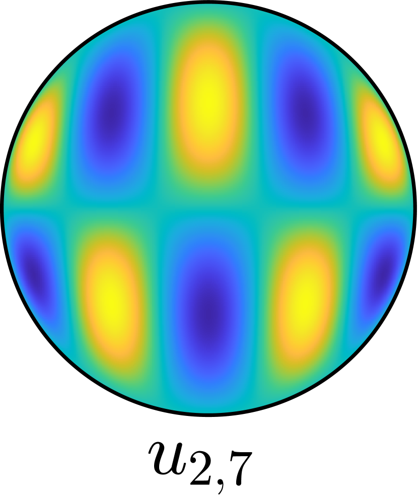
which precisely satisfies the conditions given in (4.10). Let be the Chebyshev polynomials, which are defined by . Therefore, we have solutions to the eigenvalue problem (2.1) at given by
| (4.11) |
The above forms a complete basis of since for every , the set consists of linearly independent degree polynomials vanishing at the boundary. Linear independence follows immediately from the fact that is an eigenfunction of with eigenvalue . See Figure 1. Furthermore, we see that there are infinitely many solutions to the eigenvalue problem (2.1) for every such that is rational, since there are infinitely many ways to represent a rational number as .
The explicit formulas (4.11) for the solutions of the eigenvalue problem directly completes the proof of Theorem 2 for the unit disk. The proof of Theorem 2 for ellipses and rectangles is now a purely geometric problem.
Proof of Theorem 2.
Let be an ellipse. Then there exists a symmetric nondegenerate matrix and such that where is the unit disk. Then observe that there exists a family of rotation matrices that depends smoothly on such that under the coordinate change
on becomes on , for some and smooth and monotonically increasing with and . The result then follows from the explicit basis of eigenfunctions corresponding to eigenvalues dense in given in (4.11) for the circle.
The rectangle case follows from the square case simply by a linear change of coordinates by a diagonal matrix independent of . ∎
Acknowledgements. The authors would like to thank Semyon Dyatlov, Maciej Zworski, and Leo Maas for insightful discussions. They would also like to thank Matthew Colbrook for providing the numerical data used in Figure 2. The second author is partially supported by Semyon Dyatlov’s NSF CAREER grant DMS-1749858.
References
- [Ale60] R. A. Aleksandryan. Spectral properties of operators arising from systems of differential equations of Sobolev type. Tr. Mosk. Mat. Obs., 9:455–505, 1960.
- [Arn61] V. I. Arnol’d. Small denominators I. mapping the circle onto itself. Izv. Akad. Nauk SSSR Ser. Mat., 25:21–86, 1961.
- [BR17] G. Backus and M. Rieutord. Completeness of inertial modes of an incompressible inviscid fluid in a corotating ellipsoid. Phys. Rev. E, 95:053116, May 2017.
- [Bro16] C. Brouzet. Internal wave attractors : from geometrical focusing to non-linear energy cascade and mixing. Theses, Université de Lyon, July 2016.
- [CdV20] Y. Colin de Verdière. Spectral theory of pseudodifferential operators of degree 0 and an application to forced linear waves. Analysis & PDE, 13(5):1521–1537, jul 2020.
- [CdVSR20] Y. Colin de Verdière and L. Saint-Raymond. Attractors for two-dimensional waves with homogeneous hamiltonians of degree 0. Communications on Pure and Applied Mathematics, 73(2):421–462, 2020.
- [CdVV23] Y. Colin de Verdière and J. Vidal. The spectrum of the poincaré operator in an ellipsoid, 2023. Preprint; arXiv:2305.01369.
- [CHT21] M. Colbrook, A. Horning, and A. Townsend. Computing spectral measures of self-adjoint operators. SIAM Review, 63(3):489–524, 2021.
- [Col21] M. Colbrook. Computing spectral measures and spectral types. Commun. Math. Phys., 384:433–501, 2021.
- [Col22] M. Colbrook. Specsolve: Spectral methods for spectral measures, 2022. Preprint; arXiv:2201.01314.
- [Den32] A. Denjoy. Sur les courbes definies par les équations différentielles à la surface du tore. Journal de Mathématiques Pures et Appliqués, 11:333–376, 1932.
- [dMvS93] W. de Melo and S. van Strien. One-Dimensional Dynamics. Springer Berlin, Heidelberg, 1993.
- [DWZ21] S. Dyatlov, J. Wang, and M. Zworski. Mathematics of internal waves in a 2d aquarium, 2021. Preprint; arXiv:2112.10191.
- [DZ19] S. Dyatlov and M. Zworski. Microlocal analysis of forced waves. Pure and Applied Analysis, 1(3):359–384, jul 2019.
- [GZ22] J. Galkowski and M. Zworski. Viscosity limits for zeroth-order pseudodifferential operators. Communications on Pure and Applied Mathematics, 75(8):1798–1869, 2022.
- [Her79] M. R. Herman. Sur la conjugaison differentiable des difféomorphismes du cercle a des rotations. Publ. Math. I.H.E.S., 49:5–234, 1979.
- [HTMD10] J. Hazewinkel, C. Tsimitri, L. R. M. Maas, and S. B. Dalziel. Observations on the robustness of internal wave attractors to perturbations. Physics of Fluids, 22(10):107102, 2010.
- [IJW15] D. J. Ivers, A. Jackson, and D. Winch. Enumeration, orthogonality and completeness of the incompressible coriolis modes in a sphere. Journal of Fluid Mechanics, 766:468–498, 2015.
- [Joh41] F. John. The dirichlet problem for a hyperbolic equation. American Journal of Mathematics, 63(1):141–154, 1941.
- [Li23] Z. Li. 2d internal waves in an ergodic setting, 2023. Preprint; arXiv:2301.12365.
- [Maa05] L. R. M. Maas. Wave attractors: Linear yet nonlinear. International Journal of Bifurcation and Chaos, 15(09):2757–2782, 2005.
- [MBSL97] L. R. M. Maas, D. Benielli, J. Sommeria, and F.-P. A. Lam. Observation of an internal wave attractor in a confined, stably stratified fluid. Nature, 388(6642):557–561, 1997.
- [ML95] L. R. M. Maas and F.-P. A. Lam. Geometric focusing of internal waves. Journal of Fluid Mechanics, 300:1–41, 1995.
- [Poi85] Henri Poincaré. Sur l’équilibre d’une masse fluide animée d’un mouvement de rotation. Acta Math., 7:259–380, 1885.
- [Ral73] J. V. Ralston. On stationary modes in inviscid rotating fluids. Journal of Mathematical Analysis and Applications, 44(2):366–383, 1973.
- [SE19] I. N. Sibgatullin and E. V. Ermanyuk. Internal and inertial wave attractors: A review. J Appl Mech Tech Phy, 60(2):284–302, 2019.
- [Sob54] S. L. Sobolev. On a new problem of mathematical physics. Izv. Akad. Nauk SSSR Ser. Mat., 18(1):3–50, 1954.
- [Tao19] Z. Tao. 0-th order pseudo-differential operator on the circle, 2019. to appear in Proc. Amer. Math. Soc.; arXiv:1909.06316.
- [Wal99] J. A. Walsh. The dynamics of circle homeomorphisms: a hands-on introduction. Math. Mag., 72(1):3–13, 1999.
- [Wan22] J. Wang. Dynamics of resonances for 0th order pseudodifferential operators. Commun. Math. Phys., 391:643–668, 2022.
- [Yoc84] J.-C. Yoccoz. Conjugaison différentiable des difféomorphismes du cercle dont le nombre de rotation vérifie une condition diophantienne. Annales scientifiques de l’École Normale Supérieure, 17(3):333–359, 1984.
- [Zhu22] S. Zhu. On the smoothness and regularity of the chess billiard flow and the poincaré problem, 2022. Preprint; arXiv:2210.13384.