Interfacial Magnon-Mediated Superconductivity in Twisted Bilayer Graphene
Abstract
The interfacial coupling between electrons and magnons in adjacent layers can mediate an attractive electron-electron interaction and induce superconductivity. We consider magic-angle twisted bilayer graphene sandwiched between two ferromagnetic insulators to optimize this effect. As a result, magnons induce an interlayer superconducting state characterized by -wave symmetry. We investigate two candidate ferromagnets. The van der Waals ferromagnet CrI3 stands out because it allows compression to tune the superconducting state with an exponential sensitivity. This control adds a new dimension to the tunability of twisted bilayer graphene. Our results open a new path for exploring magnon-induced superconductivity.
Heterostructures of ferromagnets (FM) and conductors are currently attracting considerable attention in spintronics. The interfacial coupling between the localized spins and itinerant electrons gives rise to intriguing phenomena such as RKKY interactions, spin-transfer, and spin-pumping [1, 2]. Furthermore, the coupling between electrons and magnons can mediate an attractive electron-electron interaction [3, 4, 5]. This effect is analogous to the electron-phonon coupling in conventional Bardeen-Cooper-Schrieffer (BCS) superconductivity [6]. Superconductivity mediated by magnons has been studied experimentally in different materials [7, 8, 9]. Furthermore, superconductivity mediated by (antiferromagnetic) magnons might also appear in certain high- superconductors [10, 11].
Superconductivity induced by interfacial coupling to magnons could exist in various material combinations. Examples are normal metals coupled to ferro- and antiferromagnets [3, 5], as well as ferromagnets and antiferromagnets coupled to the surface of topological insulators [12, 4, 13, 14]. The ferromagnetic case has also been experimentally studied [15, 16], showing a superconducting state with a critical temperature significantly higher than the intrinsic superconductivity of two materials. These studies consider either surface effects or monolayer conductors.
Systems designed for interfacial magnon-mediated superconductivity require specific properties. In general, superconducting critical temperatures are exponentially sensitive to interaction strength. In the present case, this is the magnon-mediated electron-electron interaction. Therefore, the electron states should be localized at the interface. Thus, the conducting layer should be as thin as possible yet stable. Furthermore, the electron density of states (DOS) should be large at the Fermi level. In fulfilling these conditions, twisted bilayer graphene (TBG) stands out as an ideal candidate [17].
Twisted bilayer graphene is a two-dimensional material. This renders the electron-magnon-induced effects in TBG more robust than in 3D normal metals, where interactions are constrained to the surface. The relative twist angle of the two graphene layers creates a long-period moiré pattern that, in turn, gives rise to flat electronic bands at certain magic angles [18, 19, 20]. Flat bands at the magic angles greatly enhance the electron DOS. TBG is, therefore, a laboratory for studying the transition from weak- to strong coupling superconductivity by tuning the twist angle. Graphene can couple to conventional ferromagnets [21, 22, 23]. TBG is also an interesting component of van der Waals heterostructures such as spin valves [24, 25]. Moreover, it is an intrinsic superconductor with a critical temperature of about K at half filling [26]. The underlying mechanism is still under debate, and the explanations range from phonon-mediated superconductivity [27, 28, 29, 30] to non-BCS type mechanisms [31, 32, 33].
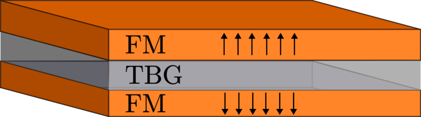
In this Letter, we consider another path to superconductivity in TBG via magnons in adjacent layers. Fig. 1 shows twisted bilayer graphene sandwiched between two identical ferromagnets with oppositely aligned magnetization. The interfacial coupling to magnons gives rise to an effective electron-electron interaction. In combination, TBG´s valley degree of freedom causes a multicomponent superconductor. We find that two of the interlayer coupling channels are suitable for Cooper pair formation. Using a BCS model, we find a -wave superconducting state with a critical temperature of the same order of magnitude as that of the intrinsic mechanism.
To describe the heterostructure, we use a Hamiltonian , where the first term describes the electrons in the twisted bilayer of graphene sheets, and the second term describes the magnons in the top and bottom layer ferromagnets. The last term describes the interfacial coupling between the ferromagnets and the graphene layers.
We consider a continuum model for the ferromagnets given by
| (1) |
where is the magnetization, is the exchange coupling, and the easy-axis anisotropy is parametrized by . A Holstein-Primakoff transformation to second order in magnon operators and a subsequent Fourier transform yields the magnon Hamiltonian
| (2) | ||||
where and are the magnon annihilation (creation) operators of momentum in the top and bottom layer, respectively. The magnon dispersion is , where is the ground state magnetization.
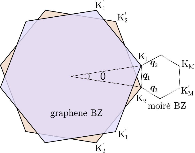
TBG consists of two graphene monolayers with a relative twist angle , as shown in Fig. 2. In the decoupled limit, the top layer has two Dirac cones and . Similarly, the bottom layer has two Dirac cones and . Because of the relative twist, the Dirac points are related by the three vectors , and . Here, is the magnitude of . The coefficient is the magnitude of the Dirac cone momenta in the monolayers. For decoupled layers, the electrons at crystal momentum near or are governed by the single layer Dirac Hamiltonian , whereas the electrons near the cones and are governed by . Here, is the Pauli matrix vector, and is the graphene Fermi velocity.
To model the low-energy electron bands of TBG, we use the Bistritzer-MacDonald Hamiltonian [20]. In the following, we present the main features required to apply the model for magnon-induced superconductivity. We start with an effective spin-degenerate Hamiltonian describing the electrons at cone and interlayer hopping in momentum space to cone . It is given by
| (3) |
The three other Hamiltonians describing electrons similarly at the cones must also be considered (see Supplemental Material). In Eq. (3), each element is a matrix in sublattice space. The Hamiltonian acts on four two-component spinors . Here, the first spinor component describes electrons near , whereas the other three components describe the electrons near . The crystal momentum , where is measured relative to the top layer‘s Dirac cone .
The Hamiltonian at couples to the Dirac cone through three hopping processes. The interlayer hopping is captured by the hopping matrices , and . The hopping strength meV [34].
The Hamiltonian in Eq. (3) exhibits low-energy eigenstates
| (4) |
where we used the shorthand notation . Projecting the Hamiltonian on these low-energy states, we get an effective sublattice space Hamiltonian on the form
| (5) | ||||
This effective Hamiltonian has the form of a single-layer Dirac Hamiltonian with a renormalized velocity
| (6) |
where . Note how yields a vanishing Fermi velocity and flat bands. This value corresponds to the largest ”magic angle.”
The Hamiltonian in Eq. (3) models electrons at cone in the top layer and three allowed interlayer hoppings to . As noted above, the related Hamiltonians for the point in the top layer and and in the bottom layer must also be considered (see Supplemental Material). Diagonalizing all four effective Dirac Hamiltonians, we find the resulting Hamiltonian
| (7) |
with a linear electron dispersion . The -operators are creation- and annihilation operators for the upper and lower bands. The eigenstates are superpositions of states at Dirac cones in both layers. Each state is ”based” at one of the four cones } with a threefold contribution from the opposing layer. The relative weight of the contributions depends on the twist angle and interlayer hopping strength . We index the eigenstates according to the cone at which it is based. Furthermore, is the spin index, and the crystal momentum is taken with respect to cone .

We model the interfacial coupling with a conventional s-d Hamiltonian
| (8) |
where is the spin operator of the itinerant electrons and is the coupling strength.
As explained above, we take into account spin fluctuations by means of a Holstein-Primakoff transformation. We only consider the interfacial coupling between the ferromagnets and their nearest graphene layer. For instance, the first component of the electron state in Eq. (4) couples to the top ferromagnetic layer, whereas the three next components couple to the bottom layer. The interfacial coupling gives rise to a layer-dependent spin splitting
| (9) |
where the spin splitting is given by
| (10) |
The layer index can be extracted directly from . It takes the value for and for . The spin index for spin up and for spin down. The spin-split electron dispersion in the moirè Brillouin zone is shown in Fig. 3. In the case of a monolayer conductor sandwiched between two oppositely aligned ferromagnets, the spin splitting vanishes exactly. This is not necessarily the case for a bilayer, as seen from Eq. (9). Each of the electron eigenstates is asymmetrically delocalized in the two layers. Hence, the net magnetic field shifts the energy of the electron states. The sign of the shift depends on spin and the layer in which the state is ”based.” At the special twist angle , the states are symmetrically distributed in the two layers such that the spin shift cancels.
We next consider the electron-magnon coupling
| (11) | ||||
The coupling parameters and depend on the index , in addition to the ferromagnetic layers and to which it couples. Their full form is given in the Supplemental material.
We derive an effective electron-electron interaction between electrons in state and via a Schrieffer-Wolff transformation [35], obtaining
| (12) |
where the interaction strength is given by
| (13) | ||||
The rich structure of Eq. (13) yields, in principle, a large number of possible pairing channels. However, not all of them are suitable for the formation of Cooper pairs. For instance, states based in the same layer with opposite spins are spin split and thus not suitable for spin-unpolarized Cooper-pairing either in the spin-singlet or spin-triplet channels. Spin-unpolarized Cooper-pairing is the only possibility when the electron-magnon coupling originates from collinear spin ground states in the magnetic insulator [36]. Hence, we focus on the coupling between electrons in different layers. This excludes half of the pairing channel candidates. Furthermore, requiring the Cooper pairs to have a zero net momentum with respect to the moiré Brillouin zone leaves two possible pairing channels. These are inter-layer intra-valley pairs denoted by
| (14) |
Within these pairing channels, the interaction can be further decomposed in terms of pairing symmetry. To that end, we approximate the magnon frequency to be constant . In this approximation, the full angular dependence originates from the coupling constants in Eq. (13). The effective interaction decomposes into an -, a -, and a -wave component. In the low-frequency limit , the - and -wave components are repulsive. In contrast, the -wave symmetry component is attractive and enables Cooper pair formation. Hence, we expect TBG to exhibit an interlayer magnon-mediated superconducting state with -wave symmetry.
We now give an estimate of the critical temperature from the conventional BCS expression
| (15) |
where is the characteristic magnon frequency. The coupling depends on the effective interaction and the DOS per valley per layer per spin. The electron DOS is enhanced near the magic angle due to the flat energy bands. Ref. [37] reports a total DOS close to the magic angle. This suggests a DOS . Although the BCS theory does not predict the critical temperature, it may be used to obtain estimates of . An important feature of Eq. (15) is the non-perturbative renormalization of the magnon energy scale, in that depends exponentially on the inverse of the DOS and the interfacial s-d coupling.
The repulsive Coulomb interaction can be detrimental to the superconducting state. TBG´s Coulomb interaction is largely screened at the magic angle for long wavelengths due to a large twist-angle dependent dielectric constant [38]. The Coulomb coupling strength is . It slightly exceeds the attractive magnon-mediated interaction. However, for two reasons, the superconducting state is robust in the presence of this Coulomb repulsion. First, the superconducting gap function is of interlayer -wave symmetry. Hence, the Cooper pairs circumvent the significant on-site -wave contribution of the Coulomb interaction. However, we will not consider the decomposition of the Coulomb interaction as the approximation is already at a crude level. Second, the Coulomb interaction is frequency independent at the scale of the magnon cut-off frequencies. To account for this, we adopt the Morel-Anderson model [39] to find an effective coupling strength
| (16) |
Here, we used the observed interband plasmon frequency as the Coulomb interaction cut off [40]. The effective interaction strength takes the value .
Interfacial coupling between graphene and ferromagnets has been studied theoretically and experimentally for numerous materials [41, 42, 22, 43, 44, 45, 46]. Hence, there are several candidates. Here, we consider two specific ferromagnets.
EuO is a ferromagnetic semiconductor with Curie temperature K. It has an fcc unit cell with lattice constant Å. Hence, two magnetic Eu2+ ions per unit cell, each with spin , are located at the interface and thus accessible for interfacial s-d coupling [47]. EuO thin films can be deposited on graphene epitaxially [41, 42]. The induced exchange splitting is found to be meV [48]. At the wave number , meV is an appropriate frequency cut-off. These parameters suggest an effective coupling strength and a critical temperature K.
CrI3 is a van der Waals ferromagnet down to the monolayer limit [49]. The crystal has two magnetic ions per unit cell. Each magnetic ion carries a magnetic moment [50]. CrI3 hosts two magnonic modes accessible for electron-magnon coupling. Their respective energies at momentum are meV and meV [51]. In a graphene-CrI3 heterostructure, CrI3 is theoretically found to induce an exchange splitting of meV [46]. Considering CrI3 as the ferromagnet, we find a coupling constant and critical temperature K.
Van der Waals ferromagnets, such as CrI3, are particularly interesting candidates. This is because the interfacial exchange splitting increases significantly under compression. For CrI3, a slight decrease in the interlayer gap can enhance the exchange splitting. A moderate reduction of the interlayer distance Å leads to an exchange splitting of 80 meV. The splitting can reach values up to 150 meV [45]. The enhanced interfacial interaction renders the higher energy magnon branch of CrI3 accessible for electron-magnon coupling. We expect this to increase the critical temperature significantly. In this way, the van der Waals spin valve exhibits a tunable compression-controlled superconducting state that connects the weak- and strong-coupling regimes. Due to the limited validity of the weak-coupling BCS model, we do not estimate the critical temperature for the compressed heterostructure.
In conclusion, we have demonstrated that interfacial magnons can induce superconductivity in twisted bilayer graphene. The magnons yield a multicomponent superconducting state due to the valley structure of TBG. We find an attractive interlayer channel suitable for Cooper pairs with -wave symmetry. Moreover, we have considered two promising candidate ferromagnets, EuO and CrI3. Both exhibit a critical temperature of the same order of magnitude as the intrinsic superconducting mechanism. Using van der Waals magnets is particularly interesting because the interlayer interaction strength is tunable through compression. For this reason, the superconducting state is tunable both via the twist angle and external compression. Twisted bilayer graphene sandwiched between ferromagnets is, therefore, a promising platform in which to explore magnon-mediated superconductivity.
The Research Council of Norway (RCN) supported this work through its Centres of Excellence funding scheme, project number 262633, ”QuSpin”, as well as RCN project number 323766.
References
- Bruno [1995] P. Bruno, Theory of interlayer magnetic coupling, Physical Review B 52, 411 (1995).
- Brataas et al. [2012] A. Brataas, A. D. Kent, and H. Ohno, Current-induced torques in magnetic materials, Nat Mater 11, 372 (2012).
- Rohling et al. [2018] N. Rohling, E. L. Fjærbu, and A. Brataas, Superconductivity induced by interfacial coupling to magnons, Physical Review B 97, 115401 (2018).
- Hugdal et al. [2018] H. G. Hugdal, S. Rex, F. S. Nogueira, and A. Sudbø, Magnon-induced superconductivity in a topological insulator coupled to ferromagnetic and antiferromagnetic insulators, Phys. Rev. B 97, 195438 (2018).
- Fjærbu et al. [2019] E. L. Fjærbu, N. Rohling, and A. Brataas, Superconductivity at metal-antiferromagnetic insulator interfaces, Physical Review B 100, 125432 (2019).
- Bardeen et al. [1957] J. Bardeen, L. N. Cooper, and J. R. Schrieffer, Theory of superconductivity, Physical review 108, 1175 (1957).
- Saxena et al. [2000] S. Saxena, P. Agarwal, K. Ahilan, F. Grosche, R. Haselwimmer, M. Steiner, E. Pugh, I. Walker, S. Julian, P. Monthoux, et al., Superconductivity on the border of itinerant-electron ferromagnetism in UGe2, Nature 406, 587 (2000).
- Aoki et al. [2001] D. Aoki, A. Huxley, E. Ressouche, D. Braithwaite, J. Flouquet, J.-P. Brison, E. Lhotel, and C. Paulsen, Coexistence of superconductivity and ferromagnetism in URhGe, Nature 413, 613 (2001).
- Pfleiderer et al. [2001] C. Pfleiderer, M. Uhlarz, S. Hayden, R. Vollmer, H. v. Löhneysen, N. Bernhoeft, and G. Lonzarich, Coexistence of superconductivity and ferromagnetism in the d-band metal ZrZn2, Nature 412, 58 (2001).
- Si et al. [2016] Q. Si, R. Yu, and E. Abrahams, High-temperature superconductivity in iron pnictides and chalcogenides, Nature Reviews Materials 1, 1 (2016).
- Lee et al. [2006] P. A. Lee, N. Nagaosa, and X.-G. Wen, Doping a Mott insulator: Physics of high-temperature superconductivity, Reviews of modern physics 78, 17 (2006).
- Kargarian et al. [2016] M. Kargarian, D. K. Efimkin, and V. Galitski, Amperean pairing at the surface of topological insulators, Physical Review Letters 117, 076806 (2016).
- Erlandsen et al. [2020] E. Erlandsen, A. Brataas, and A. Sudbø, Magnon-mediated superconductivity on the surface of a topological insulator, Physical Review B 101, 094503 (2020).
- Thingstad et al. [2021] E. Thingstad, E. Erlandsen, and A. Sudbø, Eliashberg study of superconductivity induced by interfacial coupling to antiferromagnets, Phys. Rev. B 104, 014508 (2021).
- Gong et al. [2015] X.-X. Gong, H.-X. Zhou, P.-C. Xu, D. Yue, K. Zhu, X.-F. Jin, H. Tian, G.-J. Zhao, and T.-Y. Chen, Possible p-wave superconductivity in epitaxial Bi/Ni bilayers, Chinese Physics Letters 32, 067402 (2015).
- Gong et al. [2017] X. Gong, M. Kargarian, A. Stern, D. Yue, H. Zhou, X. Jin, V. M. Galitski, V. M. Yakovenko, and J. Xia, Time-reversal symmetry-breaking superconductivity in epitaxial bismuth/nickel bilayers, Science advances 3, e1602579 (2017).
- Andrei and MacDonald [2020] E. Y. Andrei and A. H. MacDonald, Graphene bilayers with a twist, Nature materials 19, 1265 (2020).
- Li et al. [2010] G. Li, A. Luican, J. Lopes dos Santos, A. Castro Neto, A. Reina, J. Kong, and E. Andrei, Observation of van hove singularities in twisted graphene layers, Nature physics 6, 109 (2010).
- Suárez Morell et al. [2010] E. Suárez Morell, J. D. Correa, P. Vargas, M. Pacheco, and Z. Barticevic, Flat bands in slightly twisted bilayer graphene: Tight-binding calculations, Phys. Rev. B 82, 121407(R) (2010).
- Bistritzer and MacDonald [2011] R. Bistritzer and A. H. MacDonald, Moiré bands in twisted double-layer graphene, Proceedings of the National Academy of Sciences 108, 12233 (2011).
- Haugen et al. [2008] H. Haugen, D. Huertas-Hernando, and A. Brataas, Spin transport in proximity-induced ferromagnetic graphene, Phys. Rev. B 77, 115406 (2008).
- Wei et al. [2016] P. Wei, S. Lee, F. Lemaitre, L. Pinel, D. Cutaia, W. Cha, F. Katmis, Y. Zhu, D. Heiman, J. Hone, et al., Strong interfacial exchange field in the graphene/EuS heterostructure, Nature materials 15, 711 (2016).
- Wu et al. [2017] Y.-F. Wu, H.-D. Song, L. Zhang, X. Yang, Z. Ren, D. Liu, H.-C. Wu, J. Wu, J.-G. Li, Z. Jia, et al., Magnetic proximity effect in graphene coupled to a BiFeO3 nanoplate, Physical Review B 95, 195426 (2017).
- Geim and Grigorieva [2013] A. K. Geim and I. V. Grigorieva, Van der Waals heterostructures, Nature 499, 419 (2013).
- Cardoso et al. [2018] C. Cardoso, D. Soriano, N. A. García-Martínez, and J. Fernández-Rossier, Van der waals spin valves, Phys. Rev. Lett. 121, 067701 (2018).
- Cao et al. [2018] Y. Cao, V. Fatemi, S. Fang, K. Watanabe, T. Taniguchi, E. Kaxiras, and P. Jarillo-Herrero, Unconventional superconductivity in magic-angle graphene superlattices, Nature 556, 43 (2018).
- Lian et al. [2019] B. Lian, Z. Wang, and B. A. Bernevig, Twisted bilayer graphene: A phonon-driven superconductor, Phys. Rev. Lett. 122, 257002 (2019).
- Wu et al. [2018] F. Wu, A. H. MacDonald, and I. Martin, Theory of phonon-mediated superconductivity in twisted bilayer graphene, Phys. Rev. Lett. 121, 257001 (2018).
- Peltonen et al. [2018] T. J. Peltonen, R. Ojajärvi, and T. T. Heikkilä, Mean-field theory for superconductivity in twisted bilayer graphene, Physical Review B 98, 220504(R) (2018).
- Choi and Choi [2018] Y. W. Choi and H. J. Choi, Strong electron-phonon coupling, electron-hole asymmetry, and nonadiabaticity in magic-angle twisted bilayer graphene, Physical Review B 98, 241412(R) (2018).
- Oh et al. [2021] M. Oh, K. P. Nuckolls, D. Wong, R. L. Lee, X. Liu, K. Watanabe, T. Taniguchi, and A. Yazdani, Evidence for unconventional superconductivity in twisted bilayer graphene, Nature 600, 240 (2021).
- Yankowitz et al. [2019] M. Yankowitz, S. Chen, H. Polshyn, Y. Zhang, K. Watanabe, T. Taniguchi, D. Graf, A. F. Young, and C. R. Dean, Tuning superconductivity in twisted bilayer graphene, Science 363, 1059 (2019).
- Lu et al. [2019] X. Lu, P. Stepanov, W. Yang, M. Xie, M. A. Aamir, I. Das, C. Urgell, K. Watanabe, T. Taniguchi, G. Zhang, et al., Superconductors, orbital magnets and correlated states in magic-angle bilayer graphene, Nature 574, 653 (2019).
- Jung et al. [2014] J. Jung, A. Raoux, Z. Qiao, and A. H. MacDonald, Ab initio theory of moiré superlattice bands in layered two-dimensional materials, Physical Review B 89, 205414 (2014).
- Schrieffer and Wolff [1966] J. R. Schrieffer and P. A. Wolff, Relation between the Anderson and Kondo Hamiltonians, Physical Review 149, 491 (1966).
- Mæland and Sudbø [2022] K. Mæland and A. Sudbø, Topological superconductivity mediated by skyrmionic magnons, arxiv:2211.05129 (2022).
- Carr et al. [2019] S. Carr, S. Fang, Z. Zhu, and E. Kaxiras, Exact continuum model for low-energy electronic states of twisted bilayer graphene, Phys. Rev. Res. 1, 013001 (2019).
- Goodwin et al. [2019] Z. A. H. Goodwin, F. Corsetti, A. A. Mostofi, and J. Lischner, Attractive electron-electron interactions from internal screening in magic-angle twisted bilayer graphene, Phys. Rev. B 100, 235424 (2019).
- Morel and Anderson [1962a] P. Morel and P. W. Anderson, Calculation of the Superconducting State Parameters with Retarded Electron-Phonon Interaction, Phys. Rev. 125, 1263 (1962a).
- Hesp et al. [2021] N. C. Hesp, I. Torre, D. Rodan-Legrain, P. Novelli, Y. Cao, S. Carr, S. Fang, P. Stepanov, D. Barcons-Ruiz, H. Herzig Sheinfux, et al., Observation of interband collective excitations in twisted bilayer graphene, Nature Physics 17, 1162 (2021).
- Swartz et al. [2012] A. G. Swartz, P. M. Odenthal, Y. Hao, R. S. Ruoff, and R. K. Kawakami, Integration of the ferromagnetic insulator EuO onto graphene, ACS nano 6, 10063 (2012).
- Averyanov et al. [2018] D. V. Averyanov, I. S. Sokolov, A. M. Tokmachev, O. E. Parfenov, I. A. Karateev, A. N. Taldenkov, and V. G. Storchak, High-temperature magnetism in graphene induced by proximity to EuO, ACS applied materials & interfaces 10, 20767 (2018).
- Wang et al. [2015] Z. Wang, C. Tang, R. Sachs, Y. Barlas, and J. Shi, Proximity-induced ferromagnetism in graphene revealed by the anomalous Hall effect, Physical review letters 114, 016603 (2015).
- Farooq and Hong [2019] M. U. Farooq and J. Hong, Switchable valley splitting by external electric field effect in graphene/CrI3 heterostructures, npj 2D Materials and Applications 3, 1 (2019).
- Zhang et al. [2018] J. Zhang, B. Zhao, T. Zhou, Y. Xue, C. Ma, and Z. Yang, Strong magnetization and chern insulators in compressed van der waals heterostructures, Phys. Rev. B 97, 085401 (2018).
- Holmes et al. [2020] A. M. Holmes, S. Pakniyat, S. A. H. Gangaraj, F. Monticone, M. Weinert, and G. W. Hanson, Exchange splitting and exchange-induced nonreciprocal photonic behavior of graphene in CrI3-graphene van der Waals heterostructures, Physical Review B 102, 075435 (2020).
- Mauger and Godart [1986] A. Mauger and C. Godart, The magnetic, optical, and transport properties of representatives of a class of magnetic semiconductors: The europium chalcogenides, Physics Reports 141, 51 (1986).
- Yang et al. [2013] H. X. Yang, A. Hallal, D. Terrade, X. Waintal, S. Roche, and M. Chshiev, Proximity effects induced in graphene by magnetic insulators: First-principles calculations on spin filtering and exchange-splitting gaps, Phys. Rev. Lett. 110, 046603 (2013).
- Huang et al. [2017] B. Huang, G. Clark, E. Navarro-Moratalla, D. R. Klein, R. Cheng, K. L. Seyler, D. Zhong, E. Schmidgall, M. A. McGuire, D. H. Cobden, et al., Layer-dependent ferromagnetism in a van der Waals crystal down to the monolayer limit, Nature 546, 270 (2017).
- McGuire et al. [2015] M. A. McGuire, H. Dixit, V. R. Cooper, and B. C. Sales, Coupling of crystal structure and magnetism in the layered, ferromagnetic insulator CrI3, Chemistry of Materials 27, 612 (2015).
- Cenker et al. [2021] J. Cenker, B. Huang, N. Suri, P. Thijssen, A. Miller, T. Song, T. Taniguchi, K. Watanabe, M. A. McGuire, D. Xiao, et al., Direct observation of two-dimensional magnons in atomically thin CrI3, Nature Physics 17, 20 (2021).
- Morel and Anderson [1962b] P. Morel and P. W. Anderson, Calculation of the Superconducting State Parameters with Retarded Electron-Phonon Interaction, Phys. Rev. 125, 1263 (1962b).
- Dietrich et al. [1975] O. W. Dietrich, A. J. Henderson, and H. Meyer, Spin-wave analysis of specific heat and magnetization in EuO and EuS, Phys. Rev. B 12, 10.1103/PhysRevB.12.2844 (1975).
Supplemental material to ”Interfacial Magnon-Mediated Superconductivity in Twisted Bilayer Graphene”
I Ferromagnet
We consider a continuum model of magnetization dynamics in a ferromagnetic layer. The Hamiltonian is
| (S1) |
where the exchange constant , the easy-axis anisotropy and is the magnetization. We use this model for both the top and bottom ferromagnetic layers introduced in the main text. We employ the Holstein-Primakoff transformation for the variables
| (S2) |
We quantize the magnetization to quadratic order in the bosonic operators for the top layer using
| (S3) |
The ground state magnetization of the bottom layer is oppositely aligned. Hence, we quantize the operators as
| (S4) |
We consider the Hamiltonian in momentum space by using the Fourier transforms
| (S5) |
where is the area of the ferromagnet. The transformations yield the magnon Hamiltonian
| (S6) | ||||
with as stated in the main text. Here, and throughout the text, we set .
II Bistritzer-MacDonald model for TBG
A single sheet of graphene has two Dirac cones in the first Brillouin zone located at the high-symmetry points and . These cones are related by inversion symmetry and are described by Dirac Hamiltonians of opposite chirality
| (S7) |
Here, is the vector of the Pauli matrices acting on the sublattice space. In the bilayer case, we use and for the top layer and and for the bottom layer. The Bistritzer-MacDonald (BM) model describes interlayer hopping between these Dirac cones in twisted bilayer graphene [20]. The hopping from momentum relative to the cone in the top layer to the bottom layer cone is described by the Hamiltonian
| (S8) |
Here, each element is a matrix with respect to sublattice space. The vectors are defined as
| (S9) |
where the -vector magnitude is . The factor is the magnitude of the Dirac cone momenta in the single layers. The interlayer hopping matrices are , and , where is the interlayer hopping strength.
The Hamiltonian acts on the four two-component spinors . Each component is a spinor in the sublattice space. The first component is located near whereas the three components , and are located in the bottom layer near at the three distinct momenta . The crystal momentum is relative to the valley . In this basis, we project the Hamiltonian on the two-fold low-energy eigenstate
| (S10) |
where . The state is normalized to
| (S11) |
This is evident from the identity
| (S12) |
Here, denotes the identity matrix. The parameter , where is the single layer graphene Fermi velocity. Direct application of the Hamiltonian on the state in Eq. (S8) shows that the state is a zero eigenstate at and has a linear dispersion with respect to . More precisely, the projected low-energy effective Hamiltonian is
| (S13) |
where
| (S14) |
shows the twist-angle dependence of the renormalized Fermi velocity .
II.1 The full Hamiltonian
So far, we have modeled the interlayer hopping from cone to cone . In total, there are four inequivalent Dirac cones, two in each layer. In this section, we argue by symmetry to find the Hamiltonians for the three other interlayer hopping processes. We omit the spin quantum number in this section because the interlayer hopping and the Dirac Hamiltonian are spin independent.
In general, the total Hamiltonian
| (S15) |
must be invariant under the symmetries of the twisted bilayer. We relate the terms of the Hamiltonian by considering symmetry transformations that relate the cones. Ref. [27] outlines a similar procedure.
II.2 Time-reversal symmetry
We start by considering time-reversal symmetry . It relates primed and unprimed Dirac cones, such that . Furthermore, it acts as complex conjugation on the sublattice Pauli matrices. The hopping matrices transform in the following way,
| (S16) |
whereas is left invariant. The crystal momentum . In total, we have that
| (S17) |
II.3 rotation symmetry
We now use the twofold symmetry to find and . This symmetry exchanges the sublattices and flips the sign of the component. Hence,
| (S18) |
Additionally, exchanges the top and bottom layers. In total,
| (S19) |
II.4 symmetry
The combination of the symmetries yields
| (S20) |
II.5 Summary of full Hamiltonian
To summarize this section, we list the four distinct Hamiltonians
| (S21a) | |||
| (S21b) |
| (S21c) |
| (S21d) |
We can now find the low-energy eigenstates that diagonalize each of the Hamiltonians. For a compact notation, we use
| (S22) |
Inspired by Eq. (S10), we read off the normalized eigenstates directly as
| (S23a) | ||||
| (S23b) | ||||
| (S23c) | ||||
| (S23d) | ||||
Each eigenstate is taken with respect to a specific basis, i.e., the basis of the Hamiltonian, to which the eigenstate belong. For completeness, we present the bases as
| (S24a) | ||||
| (S24b) | ||||
| (S24c) | ||||
| (S24d) | ||||
II.6 The effective electron Hamiltonian
In this section, we consider the effective Hamiltonians in Eq. (II.5) with respect to their respective low-energy eigenstates given in Eq. (S23). As seen from Eq. (S13), this yields an effective model. To simplify notation, we write only the first of the two superscripts used in Eqs. (II.5) and (S23). Nevertheless, we emphasize that the eigenstates are still superpositions of electron states at cones in distinct layers. The set of effective Hamiltonians is given by
| (S25) |
Here, we introduced to account for the chirality of the Dirac cones. That is, and corresponds to the Dirac cones and , respectively. The subscript denotes the layer of the cone. The eigenvalues of the effective Hamiltonians are
| (S26) |
and the corresponding eigenvectors are
| (S27) |
Here, is the angle between and the -axis. The eigenvectors span a unitary transformation such that
| (S28) |
where
| (S29) |
Accordingly, the eigenstates in Eq. (S23) are related to band electron operators by the transformations
| (S30a) | ||||
| (S30b) | ||||
where
| (S31) |
Here, we introduced the index . It denotes at which Dirac cone each state is ”based.” Note that can be extracted directly from . The effective electron Hamiltonian for each of the cones is
| (S32) |
where denotes the energy levels and we introduced the electron spin .
III Interfacial electron-magnon coupling
In this section, we consider the s-d coupling between the ferromagnetic layers and the electrons in the graphene layers. We consider a local coupling
| (S33) |
where is the magnetization in the ferromagnet and is the spin of the itinerant electrons. We rewrite the spin operators in terms of raising and lowering operators
| (S34) |
As a result, we find
| (S35) |
We use the same Holstein-Primakoff transformation as in Eqs. (S3) and (S4) with a subsequent Fourier transform to find
| (S36a) | |||
| and | |||
| (S36b) | |||
for the top (T) and bottom layer (B). Here, and are operators of electron states located in the top and bottom layer, respectively, with momentum and spin . We use the layer indices and to emphasize that the states are not associated with particular points in the Brillouin zone. The low-energy electron states, however, are located close to the Dirac cones. We now project the Hamiltonians in Eq. (S36a) and (S36b) on the electron states given in Eq. (S24). Furthermore, we restrict our discussion to intravalley scattering. Thus, the top layer Hamiltonian can be written as
| (S37) | ||||
Here, the electron spin index is positive for spin up and negative for spin down . We now transform the coupling and project the Hamiltonian onto the low-energy states given in Eq. (S23). In this case, the coupling simplifies to
| (S38) | ||||
The bottom ferromagnet couples to the bottom graphene layer in a similar way. The explicit form is
| (S39) | ||||
The total s-d coupling is the sum of Eqs. (S38) and (S39). Note how the exchange splitting does not cancel out except at the special angle . However, this is not the magic angle . The coupling is expressed in terms of the low-energy eigenstates of the BM model. We transform the coupling using Eq. (S30), to express the coupling in terms of band electrons. To simplify the model, we consider coupling to the lower band only. In terms of lower band electron operators, the interfacial coupling is
| (S40) | ||||
The -factors can be written as
| (S41) |
The analogous coupling for the bottom layer coupling is
| (S42) | ||||
From Eq. (S40) and (S42), we can extract the exchange splitting and electron-magnon coupling constant introduced in the main text.
IV Effective interaction
The electron-magnon coupling can give rise to an effective electron-electron interaction. We consider the system Hamiltonian
| (S43) |
The electron Hamiltonian is
| (S44a) | ||||
| where we introduced the layer index . It can be extracted directly from the index , and takes the value for and for . Hence, top-layer spin-up electrons experience the same exchange spin shift as a bottom-layer spin-down electron due to the identical but anti-parallel ferromagnets. The magnitude of the spin splitting is | ||||
| (S44b) | ||||
| The electron dispersion is that of the lower band. The magnon Hamiltonian is | ||||
| (S44c) | ||||
| and the electron-magnon coupling is | ||||
| (S44d) | ||||
The coupling coefficients depend on the layer at which the electron state is based and the chirality of the Dirac cone . To account for this, we consider two disjoint subsets of . That is, we denote by and by . The coupling constants are then
| (S45a) | ||||
| (S45b) | ||||
where
| (S46) |
The and superscripts denote the top and bottom layers, respectively. The -factors are defined in Eq. (S27).
We relabel the indices of and use . The relabeling simplifies the electron-magnon coupling to
| (S47) | ||||
We split the Hamiltonian into two parts to perform the Schrieffer-Wolff transformation [35]. Let and such that we have . The small expansion parameter should not be confused with the valley index. We consider the canonical transformation
| (S48) |
and expand to find
| (S49) | ||||
To eliminate the linear term, we require
| (S50) |
To that end, we make the ansatz
| (S51) | ||||
We evaluate Eq. (S50) and find
| (S52) | ||||
where we used that . The parameters and are independent of the index to second order in the small coupling parameter . The effective interaction is
| (S53) |
The commutator has the form with containing products of fermion operators and containing sums of boson operators. The general relationship
| (S54) |
shows that there are three types of contributions. The last term represents a one-body electron operator, which can be shown to vanish [35]. The second term describes an effective coupling of an electron to two magnons. We are interested in the effective electron-electron interaction described by the first term. The magnon operators of distinct layers commute
| (S55) |
such that we can treat each layer independently to get
| (S56) | ||||
IV.1 Effective BCS type pairing
We consider a BCS-type pairing. Hence, we let . In this case,
| (S57) |
where we used that . Now, we relabel and subsequently to get
| (S58) |
The effective interaction is
| (S59) | ||||
Eq. (S58) governs the effective interaction between electrons based at Dirac cones and . Of the multiple possible channels, only a few are suitable for Cooper pair formation. We denote the partner of by and consider the pairs
| (S60) |
Note how the electron states are based in distinct layers. For this reason, they are not spin split.
For this particular choice of electron pairs, the effective interaction simplifies to
| (S61) | ||||
where
| (S62) |
The angular dependence of the effective interaction is determined by the magnon-dispersion relation and . To simplify the angular dependence, we approximate the magnon dispersion to be constant and expand
| (S63) | ||||
In the last line, we used that and have the same chirality. Eq. (S63) suggests that the effective interaction is separable with respect to angular character.
First, let such that . For this pair,
| (S64a) | ||||
| The two first terms correspond to - and -wave characters with respect to rotations in the plane. In the low-frequency limit , these channels render a repulsive interaction. Conversely, the last term yields an attractive interaction with a -wave character. Second, we consider such that . This pair yields the coupling | ||||
| (S64b) | ||||
with an attractive -wave interaction. The pairing channels and effective interactions are related through time-reversal symmetry.
V BCS gap equation
In this section, we consider the effective electron Hamiltonian.
| (S65) |
Here, the first term corresponds to the electron dispersion Eq. (S44a), including the exchange splitting effect. The second term corresponds to the effective interaction in Eq. (S58) for the pairs defined in Eq. (S60).
Following the conventional BCS approach, we introduce two hermitian conjugate gap parameters. We define
| (S66a) | |||
| (S66b) | |||
Here, is shorthand notation for . The resulting mean-field Hamiltonian is
| (S67) | ||||
To diagonalize this Hamiltonian, we introduce new fermionic operators through the Bogoliubov transformation
| (S68) |
We require the -operators to satisfy fermionic anticommutation relations
| (S69) |
which is equivalent to
| (S70) |
Furthermore, we choose and to diagonalize the Hamiltonian with respect to the quasiparticle operators. We find a special solution by choosing
| (S71) |
For this choice, the equation simplifies to
| (S72) |
Here, we used the identity , with being the opposite spin of . By squaring the equation and employing Eq. (S70), we find the relations
| (S73a) | ||||
| and | ||||
| (S73b) | ||||
The diagonal form of the Hamiltonian in Eq. (S67) is
| (S74) | ||||
The quasiparticle dispersion is spin-degenerate for this specific choice of electron pairs.
To establish the superconducting gap equation, we evaluate the expectation values in Eq. (S66b) in terms of the quasiparticle operators. We find the gap equation to be
| (S75) | ||||
The quasiparticle dispersion is given by
| (S76) |
where the layer dependent exchange splitting is for and for . We consider the gap equation for the attractive -wave channel specifically. To that end, we let with
| (S77) |
and . To estimate the order of magnitude of the critical temperature, we consider the gap equation to the second order in the small coupling parameter . In this case, the critical temperature is given by the standard expression
| (S78) |
Here, is the Boltzmann constant and where is the electron density of states.
VI Coulomb screening and candidate materials
Twisted bilayer graphene serves as an excellent candidate for exhibiting magnon-mediated superconductivity. One of the reasons is the greatly enhanced electron density of states (DOS) close to the magic angles. Ref. [37] reports a DOS over close to the magic angle. This suggests a DOS per valley per spin and per layer of .
The Coulomb interaction in momentum space is given by
| (S79) |
where is the electron charge, is the dielectric constant and is the wave vector. The repulsive interaction can be detrimental to the superconducting state. However, it is largely screened by the high DOS. Ref. [38] reports a twist-angle-dependent dielectric constant . At the magic angle, they find for long wavelengths. This gives rise to a significant screening effect. The Coulomb coupling strength for the relevant wavelengths is then
| (S80) |
The Coulomb coupling strength exceeds the attractive magnon-mediated coupling strength. However, it is effectively frequency independent at the magnon frequency cut-off. To account for this, we employ the Morel-Anderson model [52]. It effectively renormalizes the Coulomb coupling strength as
| (S81) |
Here, we used the observed interband plasmon frequency as the Coulomb interaction cut off [40]. We used meV for the magnon frequency, justified by the ferromagnets used for critical temperature estimates. The effective interaction strength takes the value . This shows that the Coulomb repulsion only weakly affects the superconducting state due to the TBG’s enhanced screening properties.
The on-site interaction is a substantial part of the repulsive Coulomb interaction. This part has an -wave symmetry. The -wave symmetry superconducting state circumvents the on-site repulsion completely, such that the Coulomb repulsion has an even weaker effect. We will not consider the decomposition of the Coulomb effect in further detail because the treatment is already at a crude level.
Interfacial coupling between graphene and ferromagnets has been studied both theoretically and experimentally for numerous materials [41, 42, 22, 43, 44, 45, 46]. Here, we consider two specific materials to give an order of magnitude estimate for the critical temperature.
EuO is a ferromagnetic semiconductor with Curie temperature K. It has an fcc unit cell with lattice constant Å. Hence, two magnetic Eu2+ ions per unit cell, each with spin , are located at the interface and thus accessible for interfacial s-d coupling [47]. EuO thin films can be deposited on graphene epitaxially [41, 42]. The induced exchange coupling is found to be meV [48]. Due to the long periodicity of the moirè structure, we consider coupling to long-wavelength magnons. Hence, we consider magnons with a wavenumber . At this momentum, the magnon dispersion is cut off at meV [53]. These parameters yield a coupling constant and a critical temperature of K when taking Coulomb interaction into account.
CrI3 is a van der Waals ferromagnet down to the monolayer limit [49]. The crystal has two magnetic ions per unit cell. Each magnetic ion carries a magnetic moment [50]. CrI3 hosts two magnonic modes accessible for electron-magnon coupling. Their respective energies at momentum are meV and meV [51]. The magnon dispersion with respect to the momentum is negligible compared to the magnon gap. Hence, we use meV. In a graphene-CrI3 heterostructure, CrI3 is theoretically found to induce an interfacial exchange splitting of meV [46]. Considering CrI3 as the ferromagnet, we find a coupling constant and critical temperature K.