Interface Dynamics in a Two-phase Tumor Growth Model
Abstract.
We study a tumor growth model in two space dimensions, where proliferation of the tumor cells leads to expansion of the tumor domain and migration of surrounding normal tissues into the exterior vacuum. The model features two moving interfaces separating the tumor, the normal tissue, and the exterior vacuum. We prove local-in-time existence and uniqueness of strong solutions for their evolution starting from a nearly radial initial configuration. It is assumed that the tumor has lower mobility than the normal tissue, which is in line with the well-known Saffman-Taylor condition in viscous fingering.
1. Introduction
In this paper, we study free boundary dynamics arising in a model of avascular tumor growth which is adapted from [1].
1.1. A two-species model of tumor growth
Consider two species of cells in , one being actively growing tumor cell and the other being inactive normal cell. Spatial densities of tumor and normal cells, each denoted by and , satisfy
| (1.1) | ||||
| (1.2) | ||||
| (1.3) |
Here denote mobilities of the tumor and normal cells. is the pressure generated by the cells, serving as a Lagrange multiplier for the constraint . It satisfies
| (1.4) | ||||
| (1.5) |
In (1.1) and (1.4), represents pressure-dependent proliferation rate of the tumor cell. In the spirit of [1], we assume that
-
(1)
.
-
(2)
is decreasing.
-
(3)
and for some .
In short, (1.1)-(1.5) models the scenario where the tumor keeps growing and where two species of cells migrate with different mobilities, according to the Darcy’s law [2], under the pressure they generate together.
Mathematical analysis of strongly-coupled competitive systems such as (1.1)-(1.5) can be challenging [3, 4, 5, 6, 7, 8]. To the best of our knowledge, existing analyses of such problems are carried out either in one space dimension or with equal mobility of the two species. In contrast, it is suggested in [1] that the cells moving with different mobilities is an important feature of the model (1.1)-(1.5). Indeed, the numerical results in [1] show that when , certain radially symmetric solution is stable, while when a Saffman-Taylor type instability [9] can occur.
1.2. A free boundary problem
In this paper, we study (1.1)-(1.5) with the restriction that and are segregated and fully saturated in their regions. Namely, we assume that and , where are two time-varying bounded domains. This gives rise to a free boundary problem that concerns dynamics of both and .
First, the equation for reduces to
| (1.6) | ||||
| (1.7) |
Then the motion law of the free boundaries are given as follows. From (1.1), we may derive the normal velocity for :
| (1.8) |
Here denotes the outward normal of with respect to . Similarly, the normal speed of is given by (1.2):
| (1.9) |
where denotes outward normal of with respect to .
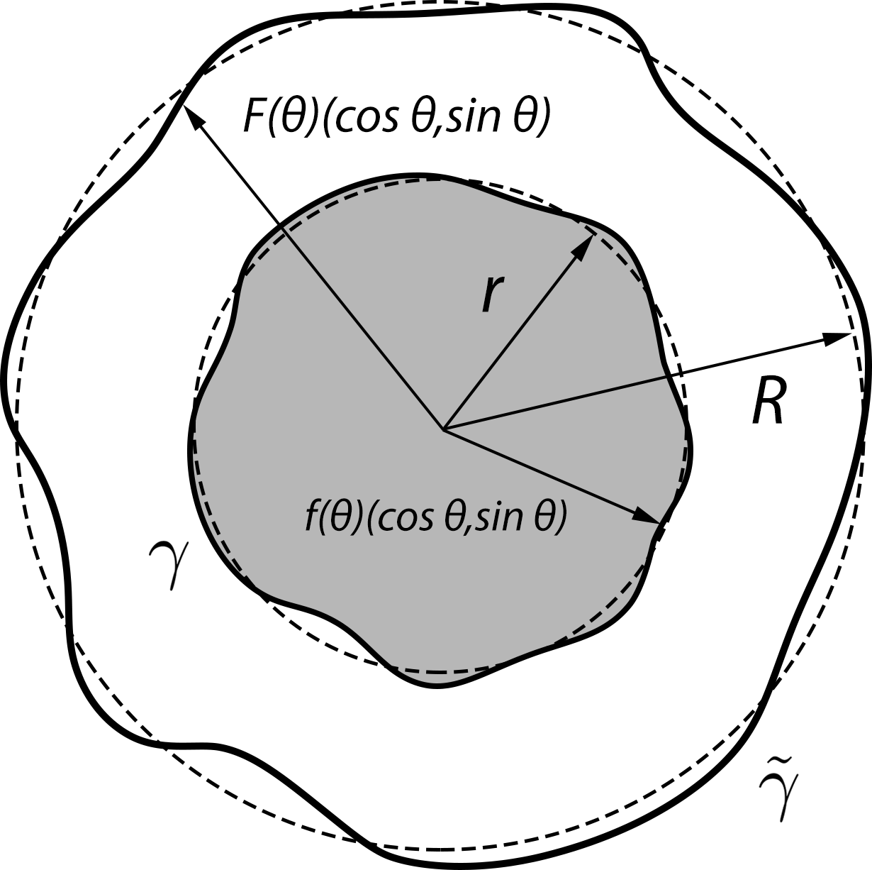
Our main result is the local-in-time well-posedness of the free boundary problem (1.6)-(1.9). Inspired by the numerical results in [1], we assume for the well-posedness. Interestingly, we will illustrate later that even with this assumption, instabilities may still occur along without further geometric assumptions on and (see Remark 2.5). We thus need to restrict ourselves to the case where the initial configuration is nearly radial (see Figure 1). More precise statement of our main results can be found in Theorem 2.1 and Theorem 2.2 in Section 2.3.
1.3. Related works and our approach
The evolution of the inner interface is similar to the 2-D Muskat problem [10, 11] with viscosity jump [12, 13], which is concerned with a close-to-flat interface between two fluids driven by the Darcy’s law. In the case when the more viscous fluid is pushed towards the less viscous one, [12] establishes global well-posedness for small initial data; in the opposite case, ill-posedness is shown. With generalized Rayleigh-Taylor condition [14], [13] formulates similar result on the well-posedness in a more general setup allowing density-viscosity jumps. Note that these rigorous results agree very well with [9] and the aforementioned numerical results in [1]. They are obtained by exploring the inherent parabolicity in the interface motion with complex analysis [12] and functional analytic [13] approaches. However, it is not clear if these approaches can be directly applied here as our model involves a geometry-dependent source term, whose support touches .
Notably there is a lot more literature concerning the Muskat problem with density jump [15, 16, 17, 18, 19] or density-viscosity jumps [20, 21, 22, 23, 13]. In both of these cases, the smoothing mechanism is essentially provided by the fact that a heavier fluid sits below a lighter one, where the gravity naturally damps the oscillation of the interface. In contrast, the smoothing mechanism is much less explicit when there is only jump in the viscosity across the interface [12, 13].
Motion of the outer interface is reminiscent of the free boundary arising in the one-phase Hele-Shaw problem [24], where a blob of fluid is injected into a Hele-Shaw cell or a porous medium and expands according to the Darcy’s law. Despite its similarity with the Muskat problem in some aspects, it admits a few other treatments. We direct the readers to [25, 26, 27, 28, 29, 30] and the references therein. Once again, in our problem, the presence of the source term depending nonlocally on and may hinder direct applications of these approaches.
In this paper, we study the dynamics of both interfaces and in a unified framework, adapted from the study of contour equations in the Muskat problem [21, 22]. We first reduce (1.6)-(1.9), which involves an elliptic equation for in a time-varying domain, partially into contour equations for the interface configurations and quantities along them; see (2.16), (2.17), (2.33) and (2.34). A key step in this reduction is to represent the transporting velocity over as a sum of three parts, which arise from the discontinuity of the cell mobilities across , the zero Dirichlet boundary condition of along , and the source term in , respectively; see (2.12) and also (2.3). Then by linearizing these contour equations around radially symmetric configurations, we show their parabolic nature under suitable conditions (c.f., Section 2.4). In particular, the interfaces can smooth themselves according to a fractional-heat-type equation with source terms. After deriving good estimates for these source terms, we prove well-posedness of the interface motion by a fixed-point argument. Smallness of the geometric deviation of and from radially symmetric configurations helps close the estimates needed in this argument. See Section 2 for more details.
1.4. Difficulties arising from the source term
This problem features a geometry-dependent source term in (1.6) that is supported up to the inner interface. It may be tempting to think of it as an innocuous regular term, but in fact, it changes the dynamics in a crucial way compared to the related problems discussed above.
Firstly, on the technical level, the source term seems to prevent the complex analysis approach in [12] from being applied here. Secondly, the parabolicity of relies on the fact that the cell with lower mobility is displacing the other species, i.e., (c.f., (1.8) and Remark 2.4), in line with the classic Saffman-Taylor condition [9]. Since depends on the domain geometry, one can manufacture such and , so that the tumor is pushed by the normal tissue along some part of under the assumption . This is possible even and both and are required to be graphs of functions over in the polar coordinate; see Remark 2.5. In this sense, simply assuming is not enough for proving well-posedness, and it is reasonable to additionally require that and are close to concentric circles (see Figure 1). Then characterization of the parabolicity of is based on a good understanding of . In Section 3, we apply elliptic regularity theory to justify that given the domain geometry close to a radially symmetric one, the corresponding should not be far away from a radially solution. That would be sufficient to guarantee parabolicity in the motion of as . Furthermore, these elliptic estimates together with the results in Section 4 and Section 5 will help justify that such parabolicity can be characterized by a fractional heat operator with exponent , which plays a central role in our analysis. See Section 2.4 and Section 8.
The source term also poses new difficulty in studying global well-posedness and stability properties near the radially symmteric solutions. Indeed, as the tumor grows larger, the pressure becomes more sensitive to the interface geometry. We demonstrate this by a scaling argument. Suppose at given time , and are close to two concentric discs, and has radius of order . Define and let and denote the corresponding dilated version of and according to the scaling. Then (1.6) becomes
| (1.10) |
with zero boundary data on , while the boundary motion laws (1.8) and (1.9) remain the same. In this new problem, the proliferation rate can have a large magnitude where is small and it is sensitive to the pressure. This results in concentration of the source term near the inner interface and a steep growth of there. On the other hand, the total mass of the normal tissue is preserved due to (1.2), and thus is extremely thin as . So in the rescaled problem the source term is close to both the inner and outer interfaces. It is then conceivable that will be highly sensitive to the domain geometry in the sense that even when the domain is pretty close to being radial, may be highly oscillatory and far from being radially symmetric. Therefore, because of the source term, nonlinear stability of the interface configurations around radially symmetric ones becomes a much more subtle issue when it comes to long time asymptotics.
1.5. Acknowledgement
This work is partially supported by National Science Foundation under Award DMS-1900804.
2. Interface Motion in an Almost Radially Symmetric Geometry
In this section, we will derive equations for the moving interfaces and in the case when they are close to concentric circles. Our main result will be established in terms of these equations. Parabolicity of these equations will be revealed, which plays a key role in proving the well-posedness.
2.1. Problem reformulation
Define a potential to be
| (2.1) |
So solves
and on . When , has discontinuity across , denoted by
(1.8) and (1.9) yield that each cell phase is transported by the velocity field . It has discontinuity across in the tangential component, but not in its normal component.
Let denote the fundamental solution of the Laplace’s equation in ,
Let denote the double layer potential operator associated with . Namely, with a boundary potential defined on , we define on to be
| (2.2) |
Note that here the gradient is taken with respect to . It is well-known that for and sufficiently smooth, say , . Then admits the following representation
| (2.3) |
where is some boundary potential defined along to be determined in order for the boundary condition , and where
| (2.4) |
Assume -regularity of and . Then the representation (2.3) along takes the average of on two sides of , i.e.,
This implies
| (2.5) |
where
On the other hand, the zero Dirichlet boundary condition of along requires that
Assuming -regularity of and , by the property of the double layer potential, should solve
along , i.e.,
| (2.6) |
2.2. Derivation of contour equations
We consider the case when and are close to two concentric circles centered at the origin, with some radii , respectively. See Figure 1. We parameterize and using the polar coordinate,
| (2.8) | ||||
| (2.9) |
where . Then and can be naturally understood as functions of . Next we shall derive equations for and (or equivalently, for and ).
Note that , where denote a vector rotated counter-clockwise by . By (2.2), all ,
| (2.10) |
By assuming ,
| (2.11) |
which is a Birkhoff-Rott-type integral [31]. Hence, by (2.3), for ,
| (2.12) |
On the other hand, by (2.7) and (2.8),
| (2.13) |
Although here should be understood as the limit of (2.12) when letting from the inside of , it is safe to simply take since the normal component of does not have discontinuity across . Define
| (2.14) | ||||
| (2.15) |
Let be defined symmetrically by interchanging and in (2.15). Thanks to (2.11) and (2.12), (2.13) can be rewritten as
| (2.16) |
Similarly,
| (2.17) |
These equations are coupled with initial conditions
| (2.18) |
For future use, we introduce
| (2.19) |
They are relative deviations of and from radially symmetric configurations.
2.3. Main results
We first introduce -space for and [32, § 2.12.2]. Let denote the Poisson semi-group on with generator . For , let
| (2.20) |
We say if and only if such that .
Our main results are as follows.
Theorem 2.1.
Suppose . Let satisfy the assumptions in Section 1. Suppose for some . Let
| (2.21) |
With be defined by (3.8), let and be negative constants
| (2.22) |
which corresponds to negative speeds of concentric circular interfaces with radii and respectively (see e.g., (3.13)). Take such that
| (2.23) |
Define and as in (2.19).
Suppose and satisfy that, with and for some ,
| (2.24) |
where is a small constant depending on , , , , , and , but not directly on . Then there exists depending on the above quantities and additionally on , such that the system (2.16)-(2.18) admits a strong solution
| (2.25) |
with for any . The solution satisfies that, with and defined in (2.19),
| (2.26) |
| (2.27) |
and
| (2.28) |
Remark 2.1.
In the claim , we did not pursue the optimal range of the Hölder exponent .
Remark 2.2.
We use to characterize the relative thinness of the gap between and . Note that requiring in (2.24) seems very natural, as otherwise the two interfaces may touch or cross each other. It is worthwhile to remark that the right hand side of (2.24) does not deteriorate as becomes smaller, in the sense that if all the model parameters and are fixed and we let (so that ), then the right hand side does not decrease to . Though also shows up on the right hand side in the form of , it will be clear later (see (8.43) in the proof of Theorem 2.1) that increases as decreases.
In contrast, the smallness of has to depend on directly: when , we may need .
Remark 2.3.
In the 2-D Muskat problem, and are considered to be critical and scaling-invariant semi-norms [22]. Although our problem does not admit any scaling law, considering its similarity with the Muskat problem, it seems to be the best thing one can do to prove well-posedness with initial data being small in - or -norms. We note that in Theorem 2.1, the condition (2.24) on the initial data is proposed in the way that, by interpolation, -semi-norms of and are small for some depending on and (see (8.25) and (8.31)). In other words, although we are not able to prove well-posedness of our problem with smallness in the “critical” spaces, partly because of the source term, we manage to do that in all the “sub-critical” cases, which can be arbitrarily close to the “critical” one — note that and are arbitrary.
Thanks to the estimates for the local solution, one can apply Theorem 2.1 iteratively and show that local solutions exist for an arbitrary time period as long as and are correspondingly sufficiently small.
Corollary 2.1.
Under the assumptions of Theorem 2.1, for any , if satisfy , where the smallness depends on , , , , , , and , the local strong solution exists up to time .
Uniqueness of local solutions can be shown if is more regular.
Theorem 2.2.
Under the assumptions of Theorem 2.1, if in addition, , then the solution is unique.
2.4. Parabolic nature of the interface motion and scheme of the proof
To elucidate the hidden parabolicity of (2.16)-(2.18), we linearize it around the radially symmetric configurations.
It is convenient to first derive equations for and by taking derivative in (2.5) and (2.6). Assuming , we have
| (2.29) |
Indeed, by integration by parts,
| (2.30) |
Here the argument is defined such that its values at coincide. In the last equality, we need the assumption . Hence, using the fact that ,
| (2.31) |
This justifies (2.29). Next let
| (2.32) |
Then and satisfy
| (2.33) | ||||
| (2.34) |
Now we shall linearize the equations (2.16), (2.17), (2.33) and (2.34) around the radially symmetric configurations, i.e., , , and . The following discussion is only formal and gives an overview of the analysis carried out in the rest of the paper. Let us begin by collecting a few facts that will be justified in later sections.
- •
- •
- •
- •
Putting these facts together, the linearized system can be written as
| (2.41) | ||||
| (2.42) | ||||
| (2.43) | ||||
| (2.44) |
Combining (2.43) and (2.41), we obtain
| (2.45) |
(2.45) is a fractional heat equation only when . Note that the last term in (2.45) and all those omitted ones are supposed to be small or regular source terms. Since , it is natural to believe that the motion of can be well-posed only when , i.e, .
Similarly, by combining (2.42) with (2.44),
| (2.46) |
Note that it shows the smoothing of the outer interface not to depend on , but only on the fact that .
Remark 2.4.
The above formal derivation may be localized as long as the interfaces are locally graphs. By doing so we may be able to show that the local parabolicity condition for the motion of is , while it is for the motion of . The former condition implies that when the less mobile cells are locally pushing the other one, we expect well-posedness in the motion of that local segment of . This is in the same spirit as the Saffman-Taylor condition [9] (see also the condition for well-posedness in [12]), and it is formulated in a more general setting in [13]. The parabolicity condition indicates that may stay regular when it is pushed towards the vacuum, but otherwise it may lose regularity. This fact echoes with many well-posedness and ill-posedness results on a variety of free boundary problems arising in, for instance, one-phase Hele-Shaw problems [25, 26, 27, 28, 29, 30] and porous medium equations [34, 35, 36, 37, 38].
Remark 2.5.
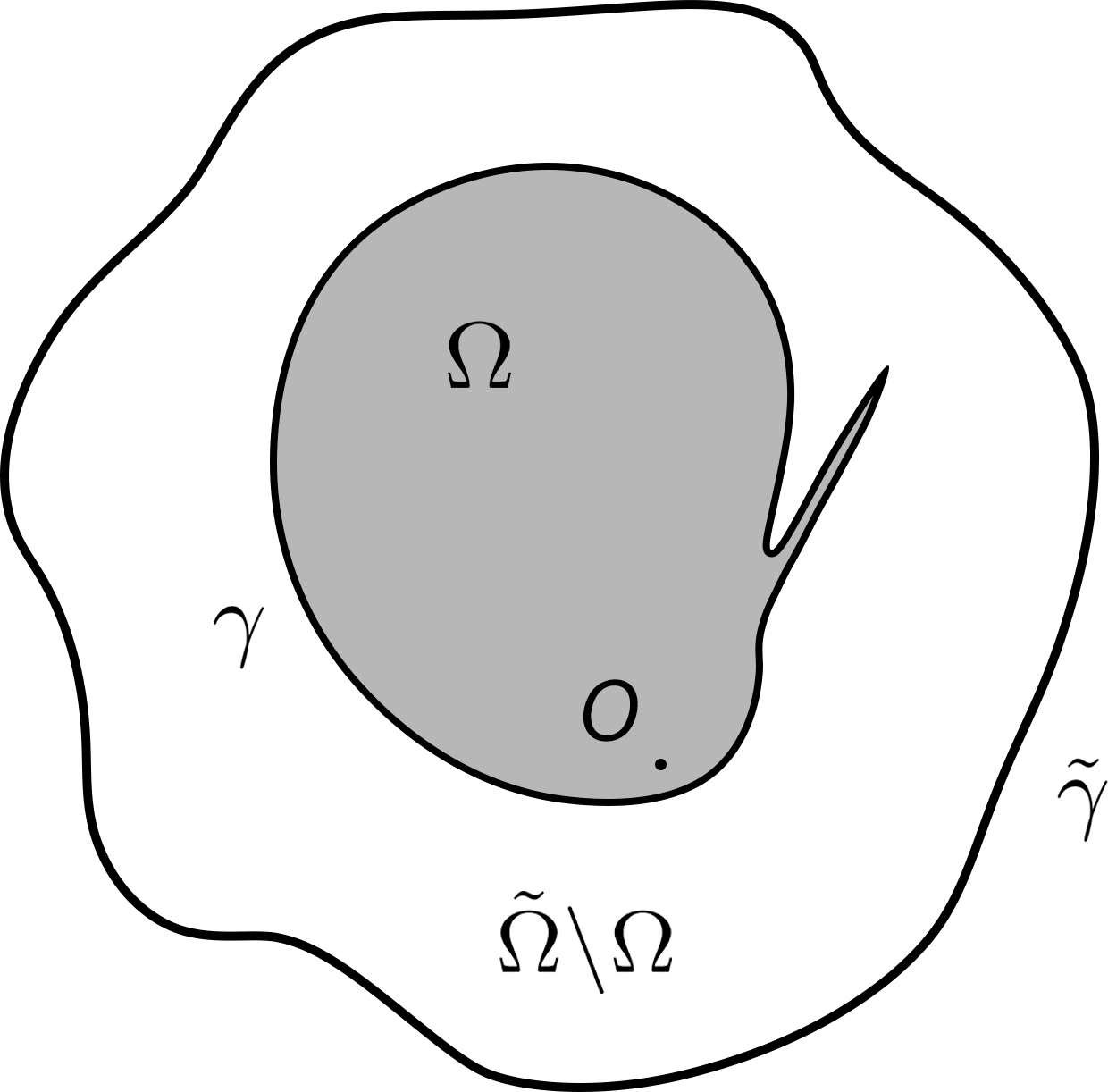
From the above discussion, we can tell that is not sufficient for the parabolicity of the motion of , since the domain geometry determines how moves in a nontrivial way. Even if both and are assumed to be star-shaped with respect to the same point, which means and can be realized as graphs of functions of in the polar coordinate, we can still manufacture such domain so that the parabolicity fails along some portion of . A possible example is shown in Figure 2, where both and are star-shaped with respect to the origin, denoted by in the figure. The tumor domain consists of a big chunk and a thin branch, where the branch is so thin that it does not significantly affect . Then it is conceivable that the thin branch will be pushed towards right under the expansion of the big chunk. So along the part of where the thin branch faces the main body of , the more mobile normal cells are pushing the less mobile tumor cells (since ), which potentially gives rise to ill-posedness of the motion of locally.
Given this, in order to guarantee well-posedness of the motion of , it is then reasonable to assume and are close to concentric circles, in which case the tumor cells should be always pushing the normal ones.
The parabolicity of (2.45) and (2.46) is sufficient to prove existence of local solutions in Section 8, and then uniqueness in Section 9. The proof of the local existence uses two layers of fixed-point arguments. We sketch it as follows.
-
(1)
Fix a pair of interface dynamics and .
-
(2)
First we need to solve for and associated with the domain defined by and . To do that, in Section 7, we apply a fixed-point argument to static equations (7.1) and (7.2) (or equivalently, (2.33) and (2.34)) with the variable . In this argument, we need estimates for the remainder terms that are omitted in (2.43) and (2.44), which turn out to be small.
-
(3)
Once and are well-defined and their estimates are derived, we use them to bound and in (2.45) and (2.46) as well as all the remainder terms omitted there (see (8.1) and (8.2) for the complete equations). They altogether will be put as the source terms in some fractional heat equations similar to (2.45) and (2.46) in order to construct a new pair of interface dynamics, and . See (8.32)-(8.34). We then show in Section 8 that the map has a fixed-point, which is a local solution.
- (4)
The proof of the uniqueness boils down to showing that , and all the remainder terms above depend in a Lipschitz manner on the interface configurations. Indeed, what we prove is a stability-type estimate for and based on that of the fractional heat equation. We carry out this idea in Section 9 with a twist in order to slightly reduce complexity of the proof.
2.5. Organization of the paper
In Section 3, we first study the pressure in an almost radially symmetric geometry by elliptic regularity theory. In Section 4, we derive estimates concerning gradients of the growth potential (c.f., (2.3) and (2.4)) restricted to inner and outer interfaces. Section 5 is devoted to proving estimates for singular integral operators and , while Section 6 establishes estimates for integral operators and . Section 7 shows well-definedness of and as well as their estimates. Finally, we prove existence of the local solution in Section 8, and uniqueness in Section 9. Some auxiliary estimates and non-essential lengthy proofs are collected in Appendices.
3. Pressure in an Almost Radially Symmetric Geometry
In this section, we focus on the elliptic equation (1.6) and (1.7) for the pressure in . The goal is to quantify the fact that if and are close to two concentric discs then should be almost radially symmetric.
3.1. Geometric preliminaries
First we introduce a diffeomorphism to transform the physical domain into a reference domain that is perfectly radially symmetric. Given satisfying (2.23), define a cut-off function , such that is only supported on , on , and for some universal constant ,
| (3.1) |
Let be a point in the reference coordinate, with . Define
| (3.2) |
where and are given in (2.19). In other words, deforms the reference domain in the radial direction only in annuli around and . It depends only on in the annulus , and only on in ; elsewhere. We may also write as . We know that is a diffeomorphism from to itself provided that is strictly increasing in for all . This is true if oscillations of and in the radial direction are small with respect to the gap between them, i.e.,
| (3.3) |
Under this assumption, it is clear that maps , , and to , , and , respectively. We denote its inverse to be .
3.2. Pressure in the reference coordinate
Define
| (3.4) |
By (1.6), in the -coordinate satisfies
| (3.5) |
Here the summation convention applies to repeated indices. We also used the notations
| (3.6) |
and
| (3.7) |
which are both functions in . We may write .
In order to show is almost radially symmetric, we shall compare it with a radially symmetric solution defined as follows.
Lemma 3.1.
Let be the -weak solution of
| (3.8) |
Then
-
(1)
is radially symmetric, i.e., , and .
-
(2)
and is decreasing in .
-
(3)
In ,
(3.9) -
(4)
For ,
(3.10) where only depends on .
-
(5)
For ,
(3.11) For ,
(3.12) Here the constants only depend on . Note that has discontinuity across , so we use to distinguish the gradients taken from two sides of .
Proof.
The radial symmetry of can be justified by a symmetrization argument in the variational formulation of (3.8). -regularity of follows from [39]. The fact that and monotonicity of follows from the maximum principle. (3.9) is obvious since is harmonic in .
To show the second bounds in (3.11) and (3.12), define to be the anti-derivative of with . Obviously, on , attaining its maximum at . Since in the polar coordinate, solves on , by multiplying with ,
| (3.14) |
Taking integral in from to yields
| (3.15) |
Hence,
| (3.16) |
By the nature of discontinuity of across , is continuous at . Hence, for , . This gives the second bound in (3.12). Finally, the second bound in (3.10) follow from (3.12), (3.13) and the fact that is increasing in .
In order to derive a bound for , we need estimates concerning and its inverse. Denote
| (3.17) | ||||
| (3.18) |
Lemma 3.2.
Suppose satisfy that . Then
| (3.19) | ||||
| (3.20) |
and
| (3.21) | ||||
| (3.22) |
The constants are all universal.
Proof.
The proof is a straightforward calculation. By (3.2),
| (3.23) |
Its inverse is given by
| (3.24) |
On the other hand, since , we deduce that
| (3.25) |
| (3.33) |
in the reference coordinate with boundary condition . Here
| (3.34) |
due to the assumptions on . Then we can prove stability of the pressure with respect to the domain geometry around the radially symmetric case.
Lemma 3.3.
Proof.
We take inner product of and (3.33) and integrate by parts,
| (3.36) |
By the definition of in (3.6), the assumptions on , Lemma 3.2 and Hölder’s inequality,
| (3.37) |
where . We proceed in two different cases.
Case 1.
Case 2.
If otherwise , by (2.23), for some universal constant . We shall first derive a bound for .
Recall that solves (1.6) and (1.7). Taking inner product of (1.6) and , we find that
| (3.40) |
where . Hence, by Lemma 3.2, in the reference coordinate,
| (3.41) |
Remark 3.1.
The above estimate involves . If , by (2.23), there exist universal constants , such that
It is noteworthy that is constant in time provided that and have sufficient regularity. This is because the transporting velocity field in is divergence-free.
3.3. More stability results
For later use, further stability results are presented here for the interface velocities and the pressure, with respect to the interface configurations.
Fix and take as in (2.23). Given two pairs of interface configurations and , let be defined as in (2.8)-(2.19). As in (3.17) and (3.18), we define and that correspond to and . We additionally introduce for some ,
| (3.45) | ||||
| (3.46) |
Also denote
| (3.47) | ||||
| (3.48) | ||||
| (3.49) | ||||
| (3.50) |
Then we can show
Lemma 3.4.
Suppose for some , satisfying that for , . Then
| (3.51) |
where . Here and are the interface velocities in the radial direction, normalized by and respectively (see (2.13).)
Let denote the pressure solving (1.6) and (1.7) on the physical domain that is determined by and , while denotes its pull back into the reference coordinate as in (3.4). An important intermediate result in proving Lemma 3.4 is the following lemma on -bound for , which will be also used when proving uniqueness of the local solution in Section 9.
Lemma 3.5.
Their proofs involve lengthy calculation, while they are relatively independent from the rest of the paper. So we leave them to Appendix B.
4. Gradient Estimates for along Interfaces
In this section, we shall derive estimates concerning and along and , where and . Aiming at greater generality, instead of working with defined in (2.4), here we shall assume for some defined in the reference coordinate and supported on , where is the inverse of defined by (3.2). We remark that the support is a slightly larger than the one corresponding to (2.4) ( in that case). The motivation for this will be clear in Section 9. Also note that .
4.1. Preliminaries
We introduce Poisson kernel on the 2-D unit disc and its conjugate :
| (4.1) | ||||
| (4.2) |
Elementary estimates for them as well as their derivatives are collected in Lemma A.1. Define
| (4.3) | ||||
| (4.4) |
See (4.43) and (4.44) for the motivation of defining these kernels. They have the following properties.
Lemma 4.1.
Let . Suppose for some and , . Here is some universal small constant, whose smallness will be clear in the proof. Then
| (4.5) |
| (4.6) |
| (4.7) |
| (4.8) |
and
| (4.9) |
Here are all universal constants. These estimates also hold if is replaced by .
Proof.
We derive that
| (4.10) |
When is suitably small, the right hand side is bounded by . This implies that are comparable with , and thus they are comparable with each other. Then (4.5) and (4.6) follow from Lemma A.1 and the assumption . Using the same facts, we can also derive that
| (4.11) |
Moreover, by Lemma A.1,
| (4.12) | ||||
| (4.13) |
Then (4.8) and (4.9) follow from
| (4.14) | ||||
| (4.15) |
The estimates for can be justified similarly. Indeed,
| (4.16) |
and
| (4.17) | ||||
| (4.18) |
Suppose the inner interface and the outer interface are defined by and through (2.8)-(2.19), respectively. Let be defined as in the beginning of Section 3. With , let
| (4.19) | ||||
| (4.20) |
Additionally, we define
| (4.21) | ||||
| (4.22) |
The motivation of introducing these quantities will be clear later in (4.43) and (4.44). In what follows, we will work with several different configurations of interfaces, determined by and , respectively. We define the corresponding quantities , , and as above, with and replaced by and .
Recall that and are defined in (3.17) and (3.18), while and are defined in (3.47) and (3.48). It is straightforward to show that
Lemma 4.2.
Suppose , with . Then with being universal constants, for all and ,
| (4.23) | ||||
| (4.24) | ||||
| (4.25) | ||||
| (4.26) |
| (4.27) | ||||
| (4.28) | ||||
| (4.29) |
| (4.30) | ||||
| (4.31) |
and
| (4.32) |
If in addition, for some , then
| (4.33) | ||||
| (4.34) |
and
| (4.35) |
Here all the constants are universal.
4.2. Estimates along
Let . With abuse of notations, let be an arbitrary point in , where the map is defined in (3.2). Then
| (4.42) |
For , . Note that the third term in (3.2) does not show up since . Then (4.42) becomes
| (4.43) |
Similarly,
| (4.44) |
We first show
Lemma 4.3.
Suppose for , such that . Let be defined in (3.47). Let be the map (3.2) determined by ( is irrelevant in this context, and one may take in (3.2) without loss of generality.) Let be its inverse. Define . Then
| (4.45) |
where is a universal constant.
In addition, satisfies an identical estimate.
Lemma 4.4.
Let such that , which defines the map in (3.2) and . Then
| (4.49) |
where is a universal constant and
| (4.50) |
Proof.
We first derive an -estimate of
| (4.51) |
which corresponds to the case . Define . Since is an odd kernel, by Hölder’s inequality and Sobolev embedding,
| (4.52) |
Now we take in Lemma 4.3 that and , and derive
| (4.53) |
Next we derive -estimates for and .
Lemma 4.5.
Proof.
Let . We take -derivative in (4.43).
| (4.57) |
Here we exchanged the integral with the -derivative, which can be justified rigorously by a limiting argument. In , an extra term is inserted without changing its value, since is odd in . When deriving , we used the fact that
| (4.58) |
and then integrated by parts. Note that it is not clear a priori whether these integrands are integrable at , so we need to write them as principal value integrals in the -variable in the first place. Yet, it will be clear in the following that all these integrands are absolutely integrable. For this reason, we omitted the notations for the principal value integral.
We start with bounding .
| (4.59) |
By Lemma 4.1, Lemma 4.2, Lemma A.1 and (4.46),
| (4.60) |
In the last inequality, when calculating the integrals, we used the facts that is supported on and that is supported on .
For and , by (4.57),
| (4.61) |
We derive in a similar manner.
| (4.62) |
By Minkowski inequality and Hölder’s inequality, with arbitrary (for definiteness, take ),
| (4.63) |
See e.g. [32, §2.5.12 and §2.7.1] for the definition of -space and the embedding of into it. Combining this with (4.57) and (4.60), we conclude with (4.56).
Lemma 4.6.
Lemma 4.7.
4.3. Estimates along
Arguing as in Lemma 4.3, we can show
Lemma 4.8.
Under the assumptions of Lemma 4.3,
| (4.74) |
where is universal. Moreover, satisfies the same estimate.
We omit its proof here, but only note that and .
Then we prove as in Lemma 4.4 that
Lemma 4.9.
Lemma 4.10.
Lemma 4.11.
5. Estimates for Singular Integral Operators and
In this section, we shall derive estimates for singular integrals of type and (see the definition in (2.14).) Singular integrals involving then follow similar estimates.
For convenience, for , denote
| (5.1) |
and
| (5.2) |
We first derive a Hölder estimate for for future use.
Lemma 5.1.
Fix . Assume , such that . Then
| (5.3) |
where .
Proof.
Using ,
| (5.4) |
With , it can be rewritten as
| (5.5) |
Since ,
| (5.6) |
By the Lipschitz continuity of on and the smallness of ,
| (5.7) |
Here we used
| (5.8) |
Take and without loss of generality. Write
| (5.9) |
We derive that
| (5.10) |
and
| (5.11) |
| (5.12) |
and similarly,
| (5.13) |
Lastly,
| (5.14) |
Note that Hilbert transform is bounded in .
Now we turn to a -estimate of .
Lemma 5.2.
Fix . Assume for some , such that with the needed smallness depending on . Then
| (5.16) |
where .
Proof.
Let and be the constants introduced in Lemma A.2 and Lemma A.4, respectively, both of which only depend on . Without loss of generality, we may assume . We also recall that is defined in (5.2).
Using the notation in (5.5), we take -derivative of to derive that
| (5.17) |
Thanks to the smallness of , we may assume . Hence, by Taylor expanding , we may rewrite in (5.5) as
| (5.18) |
By virtue of Lemma A.2,
| (5.19) |
Here is a universal constant such that . Similarly, by Lemma A.4,
| (5.20) |
Hence, with the assumption ,
| (5.21) |
To this end, by assuming , where the smallness depends on , we derive from (5.18) that
| (5.22) |
Similarly, we write
| (5.23) |
In order to bound -semi-norm of , we need an -bound of the integral above. This is possible thanks to the Hölder regularity of and . Indeed, by the mean value theorem,
| (5.24) |
Here introduced in the proof of Lemma A.2; note that . Arguing as in (5.19)-(5.21),
| (5.25) |
| (5.26) |
and hence,
| (5.27) |
By (5.23), provided that ,
| (5.28) |
We also prove a -estimate for .
Lemma 5.3.
In order to show uniqueness of the solution in Section 9, we need the following three lemmas, which are generalizations of Lemmas 5.1-5.3, respectively.
Lemma 5.4.
Lemma 5.5.
Fix and . Assume , such that with the needed smallness depending only on . Then
| (5.44) |
where .
Lemma 5.6.
6. Estimates for Integral Operators and
Recall that the integral operators and are defined in (2.15), while the Poisson kernel on the 2-D unit disc and its conjugate are defined in (4.1) and (4.2). For convenience, we denote
| (6.1) |
Lemma 6.1.
Assume , such that . Denote . Then
| (6.2) |
where is a universal constant.
Proof.
With and , we calculate that
| (6.3) |
where
| (6.4) | ||||
| (6.5) |
Here we used the fact that is an even function and has integral on . is already in the desired shape. For , since
| (6.6) |
we may assume that for some universal . Hence, by the mean value theorem and Lemma A.1,
| (6.7) |
The estimate for in (6.2) follows.
Similarly, since is an odd kernel,
| (6.8) |
where
| (6.9) | ||||
| (6.10) |
Then the estimate for in (6.2) can be derived as before.
Lemma 6.2.
Assume for some , such that . Then for ,
| (6.11) |
where .
Proof.
Let , , and be defined as in the proof of Lemma 6.1.
To handle , we first note that
| (6.15) |
We may bound the integrands in (6.15) as follows. By the mean value theorem and Lemma A.1,
| (6.16) |
where is to be determined. Here we used the bound since (see the proof of Lemma 6.1). Alternatively,
| (6.17) |
| (6.18) |
Otherwise, if , we deduce by (6.15) and (6.17) that
| (6.19) |
Recall that , so we take . Combining these estimates with the definition of in (6.12), by interpolation inequality,
| (6.20) |
Combining this with (6.12)-(6.14), we obtain that
| (6.21) |
The estimate for can be derived in the same manner.
Lemma 6.3.
Assume and for some , satisfying that . Then
| (6.22) |
where .
Proof.
Let , , and be defined as in the proof of Lemma 6.1.
We calculate that
| (6.23) |
Arguing as in (6.6) and (6.7),
| (6.24) |
For the second term in , we derive by Lemma A.1 that
| (6.25) |
Here denotes total derivative of with respect to .
We integrate by parts in . Arguing as in (6.24),
| (6.26) |
Using the fact that has mean zero on , we derive that
| (6.27) |
By Young’s inequality,
| (6.28) |
Therefore,
| (6.29) |
Next we deal with . Since
| (6.30) |
we find by Lemma A.1 that
| (6.31) |
| (6.32) |
We notice that the last term in (6.31), which has not been bounded, is in a similar form as the original . Following (6.31) and (6.32), it is not difficult to argue by induction that for all ,
| (6.33) |
Here the constants are uniformly bounded in provided the smallness of . Since , we take and obtain
| (6.34) |
can be estimated in a similar manner, so is .
Estimates for the operator can be derived in a similar manner.
Lemma 6.4.
- (1)
- (2)
-
(3)
Assume for some and , satisfying that . Then
(6.37) where .
Lastly, for those convolution terms on the left hand sides of the estimates in Lemmas 6.1-6.4, we have that
Lemma 6.5.
For , we have
| (6.40) | ||||
| (6.41) |
and
| (6.42) | ||||
| (6.43) |
where these two constants depend on . Moreover, for ,
| (6.44) | ||||
| (6.45) |
where depends on .
Proof.
It is straightforward to derive that for ,
| (6.49) |
Moreover, by Young’s inequality,
| (6.50) |
The estimates involving follows from the fact . Note that the boundedness of Hilbert transform on can be justified by that of its counterpart on with some adaptation.
7. Existence, Uniqueness and Estimates for and
This section aims at establishing well-definedness, regularity and estimates for and . The main approach is to apply a fixed-point argument to static equations (2.33) and (2.34), by using many estimates in Sections 3-6.
With the domain determined by , , and , let be defined by (3.4) and (3.5), and let the radially symmetric solution be defined as in (3.8). Recall that and are defined in (2.22). In fact, and , so their estimates can be found in Lemma 3.1. Also recall that defined in (2.38). Then thanks to Lemma A.1.
In the spirit of the linearized equations (2.43) and (2.44), we rewrite (2.33) and (2.34) as
| (7.1) | ||||
| (7.2) |
where
| (7.3) |
| (7.4) |
In what follows, we will need to apply the lemmas in Section 4 with . For that purpose, according to (4.50) and (4.76), we define
| (7.5) |
We can show the following relation between and .
Lemma 7.1.
Proposition 7.1.
Let and . Suppose , such that
| (7.9) |
where the smallness depends on , , and . Then there exist unique solving (2.33) and (2.34), or equivalently (7.1)-(7.4). They satisfy that
| (7.10) |
where .
Proof.
We will first derive a priori estimates for and , and then briefly discuss the proof of their existence and uniqueness at the end.
By Lemmas 3.3, 4.4 and 4.7 (with ), the -smoothness of and the smallness of ,
| (7.11) |
On the other hand, for , by Lemmas 5.1, 6.1, 6.2 and 6.5,
| (7.12) |
where . Hence, by (7.3), Lemma 7.1 and the fact that ,
| (7.13) |
and thus by (7.1),
| (7.14) |
where unless otherwise stated.
Similarly, by Lemmas 3.3, 4.9 and 4.12,
| (7.15) |
| (7.16) |
where . Combining them with (7.2), (7.4) and Lemma 7.1, we obtain that
| (7.17) |
and
| (7.18) |
where .
Let us briefly explain the proof of existence and uniqueness of and . Let denote the space of -functions with mean zero. Take and satisfying the assumptions. According to (7.1) and (7.2), define a map from to itself by
| (7.19) |
Thanks to the estimates above, one can easily show that the map is well-defined and it is a contraction mapping provided the smallness of and . Then the existence and uniqueness of follow.
Proposition 7.2.
Let , and . Suppose , such that
| (7.20) |
where the smallness depends on , , , and . Then and obtained in Proposition 7.1 also belong to . They satisfy
| (7.21) |
where .
Proof.
The proof is similar to that of Proposition 7.1.
Let and be defined as in (7.5). We proceed as before.
| (7.22) |
where , and by Lemma 5.2 and Lemma 6.3,
| (7.23) |
where . Combining them with (7.1) and (7.3), by Lemma 6.5 and Lemma 7.1
| (7.24) |
and thus
| (7.25) |
where unless otherwise stated.
Moreover,
| (7.26) |
where , and
| (7.27) |
where . Hence, by (7.2), (7.4), Lemma 6.5 and Lemma 7.1, with ,
| (7.28) |
and
| (7.29) |
Since and , we combine (7.25) and (7.29) to obtain that
| (7.30) |
where . Applying Proposition 7.1 yields the desired estimate.
To prove , we simply define to be the space of mean-zero -functions. One can show that the map in (7.19) is well-defined from to itself and it is a contraction mapping, provided smallness of and .
8. Local Existence
8.1. Preliminaries
Inspired by (2.45) and (2.46), we may rewrite (2.16) and (2.17) as
| (8.1) | ||||
| (8.2) |
where
| (8.3) |
and
| (8.4) |
For future use, we also denote
| (8.5) |
We need estimates for and .
Lemma 8.1.
Proof.
By (7.1), has zero integral on . By Lemma 5.3 and Lemma 7.2,
| (8.7) |
When and are Hölder continuous on and satisfies the smallness assumption, one can rigorously show that
| (8.8) |
and thus it has mean zero on . Hence, by Poincaré inequality and (8.7),
| (8.9) |
Similarly,
| (8.10) |
| (8.11) |
Finally, by Lemmas 6.1, 6.3 and 6.5,
| (8.12) |
Combining these estimates with (8.3), we obtain the estimate for in (8.6).
The estimate for can be derived in a similar manner.
We shall also need bounds for integrals of and on .
Lemma 8.2.
Proof.
We shall again use the fact that, provided , and to be Hölder continuous on ,
| (8.14) |
This is because they all can be represented as -derivatives of certain quantities as in (8.8).
Applying this fact to (8.3),
| (8.15) |
By (7.1), Poincaré inequality, Lemmas 3.3, 4.4, 5.3, 6.1, 6.5 and 7.1, as well as Propositions 7.1 and 7.2, we derive that
| (8.16) |
where .
The estimate for the can be derived similarly.
8.2. Proof of existence of local solutions
Now we are ready to show existence of local solutions.
Proof of Theorem 2.1.
The proof is an application of the Schauder fixed-point theorem.
Step 1 (Setup).
Let be chosen according to (2.23). Also recall that , and and are given in (2.24). We assume . The exact smallness of will be specified later.
With to be determined, we define
| (8.17) |
is a non-empty, convex, closed subset of . Take to be determined. Denote
| (8.18) |
By Aubin-Lions Lemma [41], the embedding
| (8.19) |
is compact, so is compact in . In what follows, we shall apply Schauder fixed-point theorem on
| (8.20) |
which is a non-empty, convex, compact subset of .
Step 2 (Estimates for elements in ).
Take . By the definition of and Lemma 3.1,
| (8.21) |
By the definition of the -seminorm in (2.20),
| (8.22) |
Moreover, [32, § 2.7], where is the closure of in the -topology. So is continuous in valued in and hence
| (8.23) |
Applying interpolation to (8.21) and (8.23) yields
| (8.24) |
Hence, taking
| (8.25) |
we find that
| (8.26) |
Step 3 (Construction of a map on ).
Inspired by (8.1) and (8.2), for given , we let solve
| (8.32) | ||||
| (8.33) |
Recall that and are defined in (8.5), which are uniquely determined by via (2.33) (c.f., Proposition 7.2), (2.34), (8.3) and (8.4). Then let
| (8.34) |
A fixed-point of the map is then a solution of (8.1) and (8.2).
We shall show that is continuous from to itself in the topology of and then apply Schauder fixed-point theorem. It suffices to prove that:
-
•
the map is well-defined as a continuous function on in the topology of , and
-
•
for properly chosen and .
Step 4 (Continuity of ).
We choose . By (8.1) and (8.2),
| (8.35) |
By (8.31) and Lemma 3.4, provided that which depends on , and , for any pair ,
| (8.36) |
where
| (8.37) |
We abbreviate it as if it incurs no confusion. By taking in (8.36) which corresponds to , we show that ; so are and . Following a similar argument, we may apply Lemma 3.4 to different time slices of and , and use the time continuity to prove .
Let be the unique solution of (8.32) and (8.33) in corresponding to . By Lemma A.7 and (8.36),
| (8.38) |
On the other hand, let . By (8.32) and (8.36),
| (8.39) |
Combining this with (8.38), we use interpolation as well as (8.21), (8.23), (8.27) and (8.29) to derive that
| (8.40) |
where . Similarly, enjoys the same bound. This proves (Hölder) continuity of in in the topology of .
In fact, if one improves Lemma A.7, it can be shown that is log-Lipschitz continuous in in the topology of . We omit the details although it may be of independent interest.
Step 5 (Justification of ).
Let be taken as before, and let . It is not difficult to show that
| (8.41) |
Combining with Lemma 8.1,
| (8.42) |
Then we derive by Lemma 3.1, Proposition 7.1, Lemma 7.2, (8.22), (8.28) and (8.31) that
| (8.43) |
where . Here we rewrote the - and -dependence into dependence on and , and used the fact that . In particular, does not deteriorate as becomes smaller. Hence,
| (8.44) |
where .
To this end, applying Lemma A.5 and Lemma A.6 to (8.32) and (8.33), we obtain that
| (8.45) |
Here the universal constant has the same dependence as above. Now we take
| (8.46) | ||||
| (8.47) |
so that (8.45) becomes
| (8.48) |
Note that the smallness needed for will not be more stringent as becomes smaller.
Finally, we show satisfies the -bound in the definition (8.17) of . By Lemma 8.2, Sobolev inequality and (8.42),
| (8.49) |
| (8.50) |
Combining this with (8.32) and (8.33), we use the fact to obtain that
| (8.51) |
where . Take in (8.47) even smaller if necessary, so that the required -bound for in (8.17) is achieved.
This shows that has its image in .
Step 6 (Existence and estimates).
8.3. Continuation of the local solutions
A local solution can be extended to longer time intervals as long as and still satisfy the smallness assumption (2.24) on the initial data. We start with the following lemma that links estimates for and when they are treated as new initial datum, with the estimates for and .
Lemma 8.3.
Under the assumptions of Theorem 2.1 with suitably small, let and be a local solution over . Define and . Let
| (8.54) |
and according to (2.19),
| (8.55) |
Let
| (8.56) |
Then , and satisfy (2.23). Moreover, with some universal constant ,
| (8.57) |
where is defined in (2.24) with , and .
Proof.
To show (8.57), we first study and . Note that (2.26) readily provides
| (8.58) |
A bound for -seminorm of and may be derived as follows. Denote and . By (8.34) and (8.48), they satisfy
| (8.59) |
and
| (8.60) |
We make zero extension of and to the region while still denote the extension to be and . Then the above properties imply that . By trace theorem (see e.g., [32, §2.7.2]) and (8.48),
| (8.61) |
It is noteworthy that the constants may only depend on but not on . On the other hand, by the definition (2.20) of the -seminorm,
| (8.62) |
Combining this with (2.24) and (8.61), we conclude that
| (8.63) |
Proof of Corollary 2.1.
We would like to construct a local solution over by making successive continuations.
Step 1 (Setup).
We can always start with and satisfying the smallness condition of Theorem 2.1. To make the notations more systematic, we rewrite , and in Theorem 2.1 as , and , respectively. Let and be defined as in (2.19). Since
| (8.68) |
where according to (8.46),
| (8.69) |
by Theorem 2.1, there exists a solution on , where by (8.47),
| (8.70) |
Define .
Suppose we have obtained a solution on for some . We define
| (8.71) |
| (8.72) |
Also let
| (8.73) |
With this choice, , and satisfy (2.23). Let and be defined by , , and as in (2.19). Then if
| (8.74) |
where
| (8.75) |
Theorem 2.1 claims that there exists a solution on , where by (8.47),
| (8.76) |
To this end, we let , and define and for . Then it is easy to verify that is a local strong solution on .
Starting from the initial data, if we are able to make such continuation until for some finite , then we prove the existence of a strong solution on . Otherwise,
-
(1)
either (8.74) is first violated for some finite (depending on the initial data) with ;
-
(2)
or we are able to make continuation for infinitely many times but still can not reach . This implies that for all , and (8.74) holds, while
(8.77)
We are going to show that both of them would not occur if we take initial datum and to be sufficiently small.
Step 2 (A priori estimates for configurations staying almost circular).
Consider an arbitrary such that and (8.74) holds for all numbers from to . We shall first derive upper and lower bounds for and .
Since (8.74) holds, in which is sufficiently small, the inner and outer interfaces at times are all sufficiently close to circles (we use the convention ). In this case, we must have as the interfaces can not cross by the proof of Theorem 2.1. Moreover, with some universal constants and ,
| (8.78) |
The increment of is due to the growth of the tumor, which provides a naive bound for
| (8.79) |
Therefore, for all such , and admit an upper bound that only depends on , and . Since the initial data is assumed to satisfy the smallness condition (8.68), is comparable with up to universal constants. Hence, the -dependence can be rewritten as -dependence. We note that Lemma 3.1 may provide a better upper bound that depends linearly on , but the naive bound here is enough for this qualitative discussion. On the other hand, because of the growth of the tumor, . This gives a positive lower bound for and that only depends on , and thus only on by the same reasoning as above.
To this end, we note that is a continuous function in . The continuity can be justified using Lemma 3.4 with and and being small constants. Indeed, is the speed of the outer interface when the interfaces are concentric circles with radii and , respectively. Therefore, for all such , admits positive lower and upper bounds depending only on , , , , and .
By Remark 3.1, has lower and upper bounds that only depend on . This together with the bound for implies that has positive lower and upper bounds only depending on , , and .
By the proof of Theorem 2.1 (c.f., (8.47) and (8.51)), has continuous dependence on , and . Combining all the facts above, there is a universal , such that for all such ,
| (8.80) |
This contradicts with (8.77), so case (2) above is ruled out.
Similarly, there exists a universal such that for all such ,
| (8.81) |
Step 3 (Estimates for total number of continuations).
It suffices to consider the case (1) above.
Thanks to (8.80), if (8.74) always holds, we only need to make continuation for finitely many times to cover the time interval . To be more precise, by choosing the longest possible lifespan of the local solution in each stage of continuation, we can have for some that admits an upper bound
| (8.82) |
provided that (8.74) is not violated along the way. In order to make (8.74) hold for times, we take sufficiently small (recall that is defined by , and in (2.24)), such that
| (8.83) |
where is given in Lemma 8.3 and is introduced in (8.81). Note that the required smallness for only depends on , , , , and . With (8.83), it is easy to justify by Lemma 8.3 that (8.74) will always be satisfied before the solution is extended beyond .
This completes the proof.
9. Uniqueness
In this section, we prove uniqueness of the local solution under the additional assumption .
9.1. Basic setup
We start with basic setups that will be used throughout this section. Let and as in Theorem 2.1, and . Let be defined in (8.25) and as in the proof of local existence (see step 5). In particular, and .
Suppose there are two solutions and of (2.16)-(2.18) with regularity and estimates given in Theorem 2.1. We define and as in (2.19). Let , , and be defined as in (3.17), (3.18), (3.45) and (3.46), respectively, and let , , and be defined in (3.47)-(3.50). By virtue of (2.26), by imposing sufficient smallness in (2.24) that depends on , and , we may assume that for all , and , and
| (9.1) |
Later we shall see the smallness needs to depend on and .
Let solve (1.6) and (1.7) in the (time-varying) physical domain that is determined by and . Let be the diffeomorphism between the physical and the (time-invariant) reference domains, determined by and via (3.2), and let be its inverse. Define as the pull-back of to the reference domain. Let be the potential defined in (2.1) corresponding to . Let and be defined as in (7.5).
The idea of proving uniqueness is to first derive bounds for and (see (8.5)) in terms of and by following the arguments in previous sections, and then use regularity theory of (8.1) and (8.2) to conclude that and can only be zero if they initially are. Such a process would be extremely involved if carried out naively, requiring more estimates than we currently have. To slightly reduce the complexity, we shall segregate inner and outer interfaces by a cut-off function in space, which decouples their dynamics in some sense.
With abuse of notation, let be a time-independent, radially symmetric, smooth cut-off function on the physical domain, such that in , on , and outside . Moreover, we need and for some universal . For , define
The equation satisfied by can be derived from (1.6), (1.7) and (2.1). Proceeding as in Section 2,
| (9.2) |
where we define in the reference coordinate
| (9.3) |
Note that the last two terms above are only supported on , where the diffeomorphism is identity. Comparing (2.3) and (9.2), we find
| (9.4) |
Hence, we claim that
| (9.5) |
Indeed, we may first assume for some boundary potential to be determined along . Then we observe and have to coincide in because of (9.4) and the fact there. Since and are harmonic inside , this proves . For convenience, we also introduce
| (9.6) |
Then (9.5) becomes
| (9.7) |
This also implies
| (9.8) |
9.2. Estimates for differences of two solutions
Next we shall bound and .
Lemma 9.1.
and are supported in , satisfying that
| (9.17) | ||||
| (9.18) |
and
| (9.19) | ||||
| (9.20) |
Proposition 9.1.
Assume (9.1) with the smallness depending on and (and thus on and .)
| (9.21) |
and
| (9.22) |
where unless otherwise stated.
Proof.
We proceed as in Proposition 7.1 and Proposition 7.2. By Lemmas 3.5, 4.3-4.7, 7.1 and 9.1,
| (9.23) |
where . Here we used the estimate by (7.5) and Lemma 3.5 that
| (9.24) |
where . Similarly,
| (9.25) |
On the other hand, by (9.1), Lemma 5.1 and Lemma 5.4,
| (9.26) |
Combining these estimates with (9.1), (9.9), (9.11) and Proposition 7.1 yields
| (9.27) |
and
| (9.28) |
where . Note that and essentially depend on and .
To show (9.22), we derive as in (7.22) that
| (9.29) |
We shall need an estimate for with explicit - and -dependence. By (9.4), and then (2.11), Lemmas 3.3, 4.4, 6.1, 6.5, 7.1 and Proposition 7.1,
| (9.30) |
Hence,
| (9.31) |
On the other hand,
| (9.32) |
and by Lemma 5.2 and Lemma 5.5,
| (9.33) |
where . Combining these estimates with (9.1), (9.9), (9.11), (9.21) as well as Propositions 7.1 and 7.2, we can show
| (9.34) |
and thus (9.22).
Proposition 9.2.
Proof.
We justify as before. By Lemmas 3.5, 4.8-4.12, 7.1 and 9.1,
| (9.37) |
where . Here we used the fact that, by (4.76), (7.5) and (9.6), with being the unit outer normal vector of ,
which yields by (9.24) that
| (9.38) |
Similarly,
| (9.39) |
Again by (9.1), Lemma 5.1 and Lemma 5.4,
| (9.40) |
By (9.12), (9.37), (9.39), (9.40) and Proposition 7.1,
| (9.41) |
Lemma 9.2.
Under the assumption of Proposition 9.1,
| (9.46) |
| (9.47) |
| (9.48) |
and
| (9.49) |
where unless otherwise stated.
Lemma 9.3.
Proof.
We argue as in Lemma 8.1. Note that has mean zero on . By Poincaré inequality and Lemmas 5.3 and 5.6,
| (9.52) |
| (9.53) | ||||
| (9.54) |
So by Proposition 7.1, Proposition 7.2 and Lemma 9.2,
| (9.55) |
where unless otherwise stated. Similarly,
| (9.56) |
By (9.24) and Lemmas 4.3-4.7 and 9.1,
| (9.57) |
and
| (9.58) |
Note that this term is not of mean zero on , so we have to bound its -norm and -seminorm in order to prove (9.50). Finally,
| (9.59) |
and by proceeding as in (9.29)-(9.31),
| (9.60) |
Combining these estimates with (9.15), we use the fact by Lemma 3.1 to prove (9.50).
9.3. Proof of the uniqueness
Now we are ready to prove uniqueness.
Proof of Theorem 2.2.
In this proof, we always assume that the constant has the dependence unless otherwise stated.
As stated at the beginning of this section, suppose there are two solutions and of (2.16)-(2.18) with regularity and estimates given in Theorem 2.1. By (9.13) and (9.14), and solve
| (9.66) | ||||
| (9.67) |
with initial condition .
Let , to be chosen. By virtue of Lemma A.5 and Lemma A.6, with ,
| (9.68) |
Here we first applied change of time variables to normalize the coefficients of fractional Laplacians in (9.66) and (9.67), and then applied Lemma A.5 and Lemma A.6 to obtain these estimates. To fulfill the condition of Lemma A.6, we need
| (9.69) |
Note that by Lemma 3.1, the right hand side is bounded from below by some constant depending only on , and .
On the other hand, by Sobolev embedding (in space) and Hölder’s inequality (in time)
| (9.70) |
Denote
| (9.71) |
By interpolation and Lemma 9.3, with ,
| (9.72) |
Here the constants and have the same dependence as introduced above.
Now we take such that and
| (9.73) |
Such relies on , , , , , , as well as the fixed solutions and . Then (9.72) becomes
| (9.74) |
In the last inequality, we used the estimate (2.26). If we assume to be suitably small, depending only on , , , , , and , we obtain that . Note that here the smallness of has no additional dependence on other parameters compared to that in the proof of existence of local solutions.
We can continue this process starting from and find a second time interval on which uniqueness holds. By repeating this argument for finitely many times (see (2.28) and the way we chose above), we can prove the uniqueness of local solution on .
Appendix A Some Auxiliary Estimates
A.1. Estimates for the Poisson kernel and its conjugate
A.2. Some Calderón-commutator-type estimates
In this part we shall establish some Calderón-commutator-type estimates used in Section 5. Recall that
| (A.17) |
Lemma A.2.
Let be a multi-index of length . Assume and for some . Define
| (A.18) | ||||
| (A.19) |
Then
| (A.20) |
where is a universal constant depending only on . Here .
Proof.
The proof essentially follows the classic argument of -boundedness of the Calderón commutator [42, ]. For completeness, we elaborate it as follows.
First we notice that is not continuous on at . For this technical reason, with abuse of notations, we introduce an even cut-off function , such that on , on , and . Write (A.18) as
| (A.21) |
It is straightforward to bound as it involves no singularity,
| (A.22) |
Here comes from the fact that
| (A.23) |
To derive an -bound for , we first show that by mathematical induction.
Step 1.
For , since is even.
Step 2.
Suppose for some and any multi-index such that , we have shown that and, with some constant that will be specified later,
| (A.24) |
It is known that the map is associated with the kernel
| (A.25) |
which is a standard anti-symmetric kernel, vanishing whenever . It can be naturally understand as a kernel on with a bound similar to (A.24). Hence, by the Theorem, it is -bounded. Its operator norm depends linearly [42, ] on the constant in (A.24) and the kernel constant of (A.25), which is bounded by
| (A.26) |
This further implies that [42, Theorem 6.6] for all satisfying , and ,
| (A.27) |
Now consider the case when . Observe that
| (A.28) |
We integrate by parts in . For almost all ,
| (A.29) |
Indeed, this can be rigorously justified by the fact that are differentiable almost everywhere. It is straightforward to derive that
| (A.30) |
On the other hand, by (A.27),
| (A.31) |
Hence, with some universal constant ,
| (A.32) |
Now assuming sufficiently large but still universal, such that
| (A.33) |
we conclude with (A.24) for . By induction, (A.24) holds for all multi-indices .
To this end, we argue as in (A.25)-(A.27) to find that is bounded from to , and also from to . By interpolation, it is -bounded as well. In particular,
| (A.34) |
Combining (A.22) and (A.34) yields a bound for that has the same form as in (A.34). A bound for can be derived easily since is an integral with no singularity.
Assuming to be even larger if needed, we obtain the desired estimate from (A.34).
Lemma A.3.
Let be a multi-index of length . With , assume that , and . Define
| (A.35) | ||||
| (A.36) |
Then
| (A.37) |
where is a universal constant depending only on .
Proof.
We shall prove (A.37) by induction. It suffices to prove it for and being smooth.
Step 1.
Step 2.
Suppose (A.37) holds for all multi-indices satisfying , where is some constant to be chosen later. Then consider the case with . By integration by parts as in (A.29), for almost all ,
| (A.41) |
By the induction hypothesis (A.37),
| (A.42) |
By Lemma A.2,
| (A.43) |
Combining these estimates with (A.41), we obtain by Sobolev embedding that
| (A.44) |
The estimate for can be derived easily, since
| (A.45) |
Taking to be suitably large, we prove (A.37) when .
This completes the proof.
Lemma A.4.
Under the hypotheses of Lemma A.2, we additionally assume and . Then
| (A.46) |
where is a universal constant depending only on .
Proof.
Instead of studying weak derivatives of and directly, we turn to difference quotients first. Without loss of generality, let be arbitrary and sufficiently small. It suffices to prove uniform-in- -bounds for and . Write
| (A.47) |
Applying Lemma A.2 and Lemma A.3,
| (A.48) |
Note that this bound is uniform in . Hence, has weak derivative, with an identical -bound as above. The estimate for can be derived similarly. Therefore, (A.46) holds if is taken to be suitably large.
A.3. Regularity theory of fractional heat equations
We focus on the following Cauchy problem of fractional heat equation on with special exponent .
| (A.49) |
For our purpose, we have that
Lemma A.5.
Lemma A.6.
Proof.
Let be the Poisson kernel on , with being the time variable, solving
| (A.52) |
in the sense of distribution. Here is the delta measure at . Note that is related to , which is defined in Section 4, in the following sense
| (A.53) |
Then can be represented by
| (A.54) |
Take arbitrary , such that . Denote . Then
| (A.55) |
By the mean value theorem, Lemma A.1 and Hölder’s inequality,
| (A.56) |
Here . Calculating the integral above yields
| (A.57) |
It is then straightforward to justify the case .
The time-continuity of in follows from the absolute continuity of the Lebesgue integral with respect to translation.
Lemma A.7.
Suppose and for some . Then for all , there exists a unique solving (A.49), satisfying that
| (A.58) |
where .
Proof.
Once again, can be represented by (A.54). It then suffices to bound its -seminorm, which also implies the uniqueness.
Finally, the time continuity of can be justified by interpolating between the facts that and for some .
Appendix B Proofs of Lemma 3.4 and Lemma 3.5
We need several preparatory results.
Let and be given as in Section 3.3. Let denote the diffeomorphism (3.2) defined by and ,
| (B.1) |
Let denote the pressure on the physical domain that is determined by and , while denotes its pull back into the reference coordinate as in (3.4). By (3.5), solves
| (B.2) |
in , with . Here is given in (3.6), and and denote -th components of and , respectively.
We first derive estimates for several ingredients in (B.2).
Lemma B.1.
Assume satisfy that . Then
| (B.3) | ||||
| (B.4) | ||||
| (B.5) |
where the constants are all universal.
If in addition, for some , such that , then
| (B.6) |
and
| (B.7) |
Here are universal constants only depending on . All the quantities above are only supported on and .
Proof.
The proof is once again a straightforward calculation.
We derive by (3.24) that
| (B.8) |
By (3.27),
| (B.9) |
Combining (3.28), (3.30) and (B.9) with (B.8), we find that
| (B.10) |
which proves (B.3). It is easy to derive (B.4) from (B.3) and Lemma 3.2.
To show (B.5), we use (3.25) to derive that
| (B.11) |
Then by (3.27), (3.28), (3.30), (3.32), (B.9) and Lemma 3.2,
| (B.12) |
To prove (B.6), we start with a Hölder estimate of . Using the fact that ,
| (B.13) |
Note that the Hölder semi-norms are taken over with respect to the Euclidean distance in -coordinate instead of the -coordinate. Using
| (B.14) |
and the fact that and are supported near and , respectively, we find that
| (B.15) |
In the last line, we applied interpolation inequalities. Setting (or ), we obtain estimates for .
Similarly, since
| (B.16) |
we deduce that
| (B.17) |
Combining (B.15) and (B.17) with (B.13) yields that
| (B.18) |
Setting gives
| (B.19) |
Thanks to (3.28), it is not difficult to derive that has the same bound, with a different constant .
Lemma B.2.
Assume with , satisfying that . Then
| (B.23) |
Proof.
By (3.5), solves
| (B.24) |
in , with . By putting in (B.4) and (B.7), we obtain that
| (B.25) | ||||
| (B.26) |
By assuming to be suitably small (ans thus is small by interpolation), we may have the coefficient matrix satisfy
| (B.27) |
which is symmetric and piecewise in . Therefore, by [39, Corollary 1.3] and Lemma 3.2, for ,
| (B.28) |
We omit the dependence of on and since they can be bounded by universal constants. The -dependence of is encoded in the -dependence. By interpolation inequality, with to be chosen and depending on and ,
| (B.29) |
Taking suitably small, we conclude from (B.28) that
| (B.30) |
Then the desired estimate follows from the fact (see Section 1).
Now we are ready to prove Lemma 3.5.
Proof of Lemma 3.5.
In this proof, we shall use to denote universal constants with the dependence . Its precise definition may vary from line to line.
Step 1 (-bound).
Rewrite (B.2) as
| (B.31) |
Arguing as in the proof of Lemma B.2, we may assume the coefficient matrix satisfies
| (B.32) |
and it is symmetric and piecewise in . Moreover,
| (B.33) |
and
| (B.34) |
Recall that . By the -bound of the weak solution [40, Theorem 8.16], together with Lemma B.1 and Lemma B.2,
| (B.35) |
This proves (3.52).
Step 2 (-bound).
This part of the proof is similar to that of Lemma B.2.
In addition to (B.32), we know that
| (B.36) |
is piecewise thanks to Lemma B.1 and Lemma B.2. Applying [39, Corollary 1.3] to (B.2), for ,
| (B.37) |
Here the constants
| (B.38) |
By (3.52), Lemma B.1 and Lemma B.2, we simplify (B.37) to be
| (B.39) |
By interpolation and arguing as in the proof of Lemma B.2,
| (B.40) |
Proof of Lemma 3.4.
Back in the physical coordinate, by (2.13),
| (B.41) |
Here is taken from the inside of . Similarly,
| (B.42) |
By definition (B.1), in a neighborhood of , while near . So (3.30) reduces to
| (B.43) |
Hence, (3.24) can be simplified as
| (B.44) |
Now we calculate by (B.41) and (B.42) that
| (B.45) | ||||
| (B.46) |
In (B.46), we used the fact that and thus is in the -direction.
To prove (3.51), we start with the trivial bound
| (B.47) |
due to the smallness of , where is a universal constant. Then we simply use to derive that
| (B.48) |
Similarly,
| (B.49) |
Setting or above yields
| (B.50) |
Then it is not difficult to derive from (B.45) that
| (B.51) |
| (B.52) |
where . Once again, the dependence of on is omitted since it is assumed to be small.
Estimates for can be derived from (B.46) in a similar manner.
Appendix C Proofs of Lemmas 5.4-5.6
Proof of Lemma 5.4.
Let be defined as in (5.2) corresponding to . By virtue of (5.5),
| (C.1) |
We start with the integrand of .
| (C.2) |
We derive that
| (C.3) |
and
| (C.4) |
Taking in the second last step of (C.4) yields that
| (C.5) |
Combining these estimates with (C.2), we argue as in (5.6) that
| (C.6) |
| (C.8) |
In order to apply the same argument to , we need the following estimate.
| (C.9) |
Since
| (C.10) |
we apply this and (C.3) to (C.9) to conclude that
| (C.11) |
Now we proceed as in (5.9)-(5.15).
| (C.12) |
By (5.11), (5.14), (C.3)-(C.6) and (C.11),
| (C.13) |
Proof of Lemma 5.5.
Let and be the constants in Lemma A.2 and Lemma A.4, respectively, both of which only depend on . Without loss of generality, we may assume . Following (5.5), we use to denote the corresponding quantities defined by . are defined as in (5.2) by . Thanks to the smallness of , we may assume , and that is a universal constant such that .
We start with bounding . Taking their -derivatives, we use (C.3) to derive that
| (C.14) |
As in (5.18), we Taylor expand and rewrite as
| (C.15) |
We derive
| (C.16) |
Note that here in this proof, with abuse of notations, we use as a summation index, which has nothing to do with (5.2).
By Lemma A.2, for ,
| (C.17) |
Letting and replacing by ,
| (C.18) |
Further taking and , we find
| (C.19) |
Similarly,
| (C.20) |
On the other hand, by Lemma A.4, for ,
| (C.21) |
Taking and replacing by ,
| (C.22) |
Further taking and ,
| (C.23) |
Similarly,
| (C.24) |
We similarly write
| (C.27) |
and
| (C.28) |
where
| (C.29) |
To proceed as before, we need -bounds for the integrals in (C.28). We additionally define
| (C.30) |
It is easy to show that , where is introduced in the proof of Lemma A.2, and
| (C.31) |
Hence, by the mean value theorem,
| (C.32) |
We also derive that
| (C.33) |
Write
| (C.34) |
Since
| (C.35) |
we use (C.10) and (C.31) to derive that
| (C.36) |
Combining this with (C.31) and (C.34) yields that
| (C.37) |
Applying this to (C.33), we obtain that
| (C.38) |
To this end, by (C.28),
| (C.47) |
For , this can be simplified as
| (C.48) |
For , by applying (C.32), (C.38), (C.40), (C.42), (C.44) and (C.46) to (C.47), we derive that
| (C.49) |
This together with (C.48) and the smallness of implies
| (C.50) |
Proof of Lemma 5.6.
Following (5.31), we use to denote the corresponding quantities defined by .
Using (5.32), we find that
| (C.51) |
It is not difficult to show by (C.3) that
| (C.52) |
Taking yields ; here we used the fact . Substituting these estimates as well as (5.17) and (C.14) into (C.51), we obtain that
| (C.53) |
To bound , we are going to make use of the estimates for in Lemma 5.5, since coincides with if in the definition of is replaced by . For this purpose, an -estimate for is needed. We start with
| (C.54) |
It is straightforward to bound the first term.
| (C.55) |
To bound the second term in (C.54), we first note that (C.32) and (C.38) still hold if in their denominators are replaced by . Hence, we argue as in the proof of Lemma 5.5 by Taylor expanding that
| (C.56) |
Taking here yields
| (C.57) |
which further implies
| (C.58) |
To this end, we may bound the second term in (C.54) as follows
| (C.59) |
Combining this with (C.54) and (C.55),
| (C.60) |
Setting (or ) provides
| (C.61) |
To emphasize the -dependence of , we shall rewrite as . Since , we derive with (C.26), (C.60) and (C.61) that
| (C.62) |
This gives
| (C.63) |
References
- [1] Tommaso Lorenzi, Alexander Lorz, and Benoît Perthame. On interfaces between cell populations with different mobilities. Kinetic and Related Models, 10(1):299–311, 2017.
- [2] HM Byrne and Mark AJ Chaplain. Modelling the role of cell-cell adhesion in the growth and development of carcinomas. Mathematical and Computer Modelling, 24(12):1–17, 1996.
- [3] Inwon Kim and Alpár Richárd Mészáros. On nonlinear cross-diffusion systems: an optimal transport approach. Calculus of Variations and Partial Differential Equations, 57(3):79, 2018.
- [4] Federica Bubba, Benoît Perthame, Camille Pouchol, and Markus Schmidtchen. Hele-Shaw limit for a system of two reaction-(cross-)diffusion equations for living tissues. arXiv preprint arXiv:1901.01692, 2019.
- [5] Piotr Gwiazda, Benoît Perthame, and Agnieszka Świerczewska-Gwiazda. A two-species hyperbolic-parabolic model of tissue growth. Communications in Partial Differential Equations, 44(12):1605–1618, 2019.
- [6] M. Bertsch, M. E. Gurtin, D. Hilhorst, and L.A. Peletier. On interacting populations that disperse to avoid crowding: preservation of segregation. Journal of Mathematical Biology, 23:1–13, 1985.
- [7] Michiel Bertsch, Roberta Dal Passo, and Masayasu Mimura. A free boundary problem arising in a simplified tumour growth model of contact inhibition. Interfaces and Free Boundaries, 12(2):235–250, 2010.
- [8] José A Carrillo, Simone Fagioli, Filippo Santambrogio, and Markus Schmidtchen. Splitting schemes and segregation in reaction cross-diffusion systems. SIAM Journal on Mathematical Analysis, 50(5):5695–5718, 2018.
- [9] Philip Geoffrey Saffman and Geoffrey Ingram Taylor. The penetration of a fluid into a porous medium or Hele-Shaw cell containing a more viscous liquid. Proceedings of the Royal Society of London. Series A. Mathematical and Physical Sciences, 245(1242):312–329, 1958.
- [10] Morris Muskat. Two fluid systems in porous media. the encroachment of water into an oil sand. Physics, 5(9):250–264, 1934.
- [11] Jacob Bear. Dynamics of fluids in porous media. Courier Corporation, 2013.
- [12] Michael Siegel, Russel E Caflisch, and Sam Howison. Global existence, singular solutions, and ill-posedness for the Muskat problem. Communications on Pure and Applied Mathematics, 57(10):1374–1411, 2004.
- [13] Bogdan-Vasile Matioc. Well-posedness and stability results for some periodic Muskat problems. arXiv preprint arXiv:1804.10403, 2018.
- [14] Joachim Escher, Anca-Voichita Matioc, and Bogdan-Vasile Matioc. A generalized Rayleigh-Taylor condition for the Muskat problem. Nonlinearity, 25(1):73, 2011.
- [15] David M Ambrose. Well-posedness of two-phase Hele-Shaw flow without surface tension. European Journal of Applied Mathematics, 15(5):597–607, 2004.
- [16] Diego Córdoba and Francisco Gancedo. Contour dynamics of incompressible 3-D fluids in a porous medium with different densities. Communications in Mathematical Physics, 273(2):445–471, 2007.
- [17] Peter Constantin, Diego Córdoba, Francisco Gancedo, and Robert M Strain. On the global existence for the Muskat problem. Journal of the European Mathematical Society, 15(1):201–227, 2012.
- [18] Peter Constantin, Diego Córdoba, Francisco Gancedo, Luis Rodríguez-Piazza, and Robert M Strain. On the Muskat problem: global in time results in 2D and 3D. American Journal of Mathematics, 138(6):1455–1494, 2016.
- [19] Diego Cordoba and Omar Lazar. Global well-posedness for the 2D stable Muskat problem in . arXiv preprint arXiv:1803.07528, 2018.
- [20] Antonio Córdoba, Diego Córdoba, and Francisco Gancedo. Interface evolution: the Hele-Shaw and Muskat problems. Annals of mathematics, pages 477–542, 2011.
- [21] Antonio Córdoba, Diego Córdoba, and Francisco Gancedo. Porous media: the Muskat problem in three dimensions. Analysis & PDE, 6(2):447–497, 2013.
- [22] Francisco Gancedo, Eduardo Garcia-Juarez, Neel Patel, and Robert M Strain. On the Muskat problem with viscosity jump: Global in time results. Advances in Mathematics, 345:552–597, 2019.
- [23] CH Arthur Cheng, Rafael Granero-Belinchón, and Steve Shkoller. Well-posedness of the Muskat problem with initial data. Advances in Mathematics, 286:32–104, 2016.
- [24] Stanley Richardson. Hele Shaw flows with a free boundary produced by the injection of fluid into a narrow channel. Journal of Fluid Mechanics, 56(4):609–618, 1972.
- [25] Charles M Elliott and Vladimır Janovskỳ. A variational inequality approach to Hele-Shaw flow with a moving boundary. Proceedings of the Royal Society of Edinburgh Section A: Mathematics, 88(1-2):93–107, 1981.
- [26] Emmanuele DiBenedetto and Avner Friedman. The ill-posed Hele-Shaw model and the stefan problem for supercooled water. Transactions of the American Mathematical Society, 282(1):183–204, 1984.
- [27] SD Howison. Complex variable methods in Hele-Shaw moving boundary problems. European Journal of Applied Mathematics, 3(3):209–224, 1992.
- [28] Joachim Escher and Gieri Simonett. Classical solutions of multidimensional Hele-Shaw models. SIAM Journal on Mathematical Analysis, 28(5):1028–1047, 1997.
- [29] Inwon C Kim. Uniqueness and existence results on the Hele-Shaw and the Stefan problems. Archive for Rational Mechanics & Analysis, 168(4), 2003.
- [30] CH Cheng, Daniel Coutand, and Steve Shkoller. Global existence and decay for solutions of the Hele-Shaw flow with injection. arXiv preprint arXiv:1208.6213, 2012.
- [31] Andrew J Majda and Andrea L Bertozzi. Vorticity and incompressible flow, volume 27. Cambridge university press, 2002.
- [32] H. Triebel. Theory of Function Spaces. Modern Birkhäuser Classics. Springer Basel, 2010.
- [33] Loukas Grafakos. Classical Fourier analysis, volume 2. Springer, 2008.
- [34] Luis A Caffarelli and Avner Friedman. Regularity of the free boundary of a gas flow in an -dimensional porous medium. Indiana University Mathematics Journal, 29(3):361–391, 1980.
- [35] Luis A Caffarelli, Juan Luis Vázquez, and Noemı Irene Wolanski. Lipschitz continuity of solutions and interfaces of the -dimensional porous medium equation. Indiana University mathematics journal, 36(2):373–401, 1987.
- [36] Luis A Caffarelli and Noemi I Wolanski. regularity of the free boundary for the -dimensional porous media equation. Communications on pure and applied mathematics, 43(7):885–902, 1990.
- [37] Juan Luis Vázquez. The porous medium equation: mathematical theory. Oxford University Press, 2007.
- [38] Inwon Kim and Yuming Paul Zhang. Porous medium equation with a drift: Free boundary regularity. arXiv preprint arXiv:1812.08770, 2018.
- [39] Yan-Yan Li and Michael Vogelius. Gradient estimates for solutions to divergence form elliptic equations with discontinuous coefficients. Archive for Rational Mechanics and Analysis, 153(2):91–151, 2000.
- [40] David Gilbarg and Neil S Trudinger. Elliptic partial differential equations of second order. springer, 2015.
- [41] Roger Temam. Navier-Stokes equations, volume 2. North-Holland Amsterdam, 1984.
- [42] Javier Duoandikoetxea. Fourier analysis, volume 29. American Mathematical Soc., 2001.
- [43] Damien Lamberton. Equations d’évolution linéaires associées à des semi-groupes de contractions dans les espaces . Journal of Functional Analysis, 72(2):252–262, 1987.
- [44] Umberto Biccari, Mahamadi Warma, and Enrique Zuazua. Local regularity for fractional heat equations. In Recent Advances in PDEs: Analysis, Numerics and Control, pages 233–249. Springer, 2018.