Interacting 1D Chiral Fermions with Pairing: Transition from Integrable to Chaotic
Abstract
We study a generic one-dimensonal quantum model of two flavors (pseudospins) chiral complex fermions by exact diagonalization, which can have local interflavor interaction and superconducting pairings (with all irrelevant terms ignored). Analytically, the model has two solvable (integrable) points in the parameter space: it is a free fermion model when the fermion interaction is zero, and is a free boson Luttinger liquid when there is a global U(1)U(1)(↓) symmetry (with nonzero interaction). When the global symmetry of the interacting model is lowered by turning on symmetry breaking parameters, the model undergoes a transition from a quantum integrable model to a fully quantum chaotic model, as we demonstrate by examining the level spacing statistics (LSS) of the many-body energy spectrum. In particular, there is a possibly integrable regime with intermediate global symmetries, where the model is neither free bosons nor free fermions, but shows Poisson LSS in each global symmetry charge sector. This implies the existence of hidden (quasi)local conserved quantities. When the global symmetries are further lowered, the LSS in each charge sector becomes Wigner-Dyson, implying quantum chaos.
I Introduction
The study of the integrability of one-dimensional (1D) interacting quantum models has a long history in condensed matter physics. The earliest such exact solution studies date back to the Bethe ansatz for the 1D Heisenberg model bethe1931 and the Onsager solution for the 2D classical Ising model (which is equivalent to a 1D quantum Ising model) onsager1944 . The successive studies in the later decades have revealed many more integrable 1D quantum models, such as the Lieb-Liniger model of 1D Bose gas lieb1963a ; lieb1963b , 1D Hubbard model lieb1968 , spin models obeying the Yang-Baxter equation mcguire1964 ; yang1967 ; baxter1971 , and the Luttinger liquid of interacting fermions Dzyaloshinski1996 ; Haldane_1981 ; Haldane1981 ; Tomonaga1950 ; Luttinger1963 ; Wen1 ; Wen2 . In particular, Chen-Ning Yang has made significant contributions to the understanding of thermodynamic behaviors of the integrable spin models yang1952 ; yang1966a ; yang1966b ; yang1966c ; yang1966d , interacting gases yang1969 in 1D, and the Yang-Baxter equation named partly after him as a sufficient condition for integrability yang1967 . These developments have significantly advanced the physicists’ understanding of quantum integrability, phase transitions and non-equilibrium quantum dynamics rigol2007 ; rigol2008 in 1D systems.
On the other hand, the study of many-body quantum chaos has recently attracted extensive interests. In contrast to quantum integrable models which have enormous number of local or quasilocal conserved quantities tetelman1981 ; grabowski1995 ; ilievski2015 ; nozawa2020 ; lian2022conserv , many-body quantum chaotic systems are expected to have limited number of local conserved quantities (from global symmetries, etc). A class of extensively studied quantum chaotic models is the Sachdev-Ye-Kitaev (SYK) type models sachdev1992fk ; polchinski2016xgd ; maldacena2016hyu ; kitaev2017awl ; lian2019 ; hu2021chiral , which are exactly solvable in the large limit, where is usually the number of flavors of particles in the model. An indication of the quantum chaos in the SYK models is the positive Lyapunov exponent in the out-of-time-ordered correlation (OTOC) in the large limit, which has a quantum upper bound at temperature Maldacena:2015waa . Moreover, quantum chaotic systems are expected to show Wigner-Dyson level spacing statistics (LSS) in each symmetry sector of the many-body energy spectrum Bohigas1984 ; Dyson1970 ; Wigner1967 , and usually satisfy the eigenstate thermalization hypothesis (ETH) jensen1985 ; deutsch1991 ; srednicki1994 ; dalessio2016 . In contrast, integrable systems generically show Poisson LSS Berry1977 , and violates the ETH.
The scope of this paper is to investigate the integrability and chaos of 1D chiral quantum models, by examining a simplest physical example of chiral fermions. 1D chiral systems constitute a significant class of 1D quantum models, which cannot exist in 1D materials, but can arise as the edge states of 2D gapped chiral topological phases of matter, such as the fractional quantum Hall (FQH) states. In the absence of spatial disorders, a big portion of such chiral models are described by the free boson chiral Luttinger liquid theory Wen1 ; Wen2 or free chiral Majorana fermions moore1991 ; wen1991 . In 1D chiral models which are not purely chiral (namely, having inequivalent modes propagating in both directions), the symmetry allowed interactions may lead to mode reconstructions under renormalization haldane1995 ; Kane1994 ; Levin2007 ; Lee2007 ; levin2013 ; wangjuven2015 ; Lian2018 ; Chamon1994 ; Wan2002 ; Wan2003 ; Sabo2017 ; Cano2014 , altering the low energy physics. For purely chiral 1D models, the recent studies have revealed a different type of mode reconstruction: the interaction may drive a transition from integrable regimes with well-defined quasiparticles to quantum chaotic regimes without low-energy quasiparticle lian2019 ; hu2021chiral ; hu2021integrability . In particular, purely chiral models can have exactly marginal interactions which do not flow under renormalization group, making the physics independent of energy scale.
A prototypical example is the chiral SYK model of flavors of chiral Majorana fermions (), which has an action lian2019
| (1) |
The interactions can be taken arbitrarily, and are exactly marginal. For , it is shown that the model with any interactions can be exactly solved as a free boson chiral Luttinger liquid (by choosing a proper Majorana fermion basis), thus is integrable. For , it is conjectured that the model becomes quantum chaotic and has no quasiparticles. In the large limit, the quantum chaos can be shown explicitly analytically by expansion techniques polchinski2016xgd ; maldacena2016hyu ; kitaev2017awl ; lian2019 : by assuming are randomly uncorrelated and , the velocity-dependent Lyapunov exponent of the OTOC is positive along all velocities within the chiral causality cone of the model, and approaches the maximal chaos bound when approaches the upper-bound for preserving the chirality (ground state stability).
Such transitions between integrable and chaotic regimes can also arise in 1D chiral models supporting anyons, for instance, in copies of Wess-Zumino-Witten (WZW) theories with current-current interactions hu2021chiral . Moreover, some chiral models can also exhibit properties between the free integrable cases (free bosons or free fermions) and the fully quantum chaotic cases, such as possibly integrable LSS behaviors hu2021integrability , and quantum scars schindler2021exact ; martin2021scar . For instance, the interacting chiral edge states of the FQH state is recently numerically found to have Poisson LSS in each conserved global symmetry charge sector hu2021integrability , indicating the existence of hidden (quasi)local conserved charges and the possibility that the model is integrable. Physically, the low-energy integrability of the chiral edge states is relevant in the detection of their quantum coherent interferences Willett2009 ; Zhao2020 ; Lian2016 ; Roulleau2008 , for instance, in the Fabry-Pérot interferometer experiment of the FQH state Laughlin1983 ; Nakamura2020 ; Carrega2021 ; McClure2012 ; Ofek2010 ; Halperin2011 . On the contrary, the quantum chaos of chiral edge states are significant for their thermal equilibration in thermal transports Banerjee2018 ; Feldman2018 ; Simon2018 ; Ma2019 .
In this paper, we employ the exact diagonalization (ED) numerical method to explore the LSS of the many-body spectrum of a generic interacting model of two flavors of chiral complex fermions, with possible superconducting pairings, and all the irrelevant terms are ignored. The model has two analytically solvable regimes in its parameter space: the free fermion regime when the interaction is zero, and the free boson regime solvable via bosonization as a chiral Luttinger liquid. With generic parameters, we find the LSS of the interacting model in each global symmetry sector undergoes a transition from Poisson to Wigner-Dyson with respect to the global symmetry, as summarized in Fig. 10. Particularly, there is a possibly integrable regime with Poisson LSS but with no free picture, which implies the existence of hidden (quasi)local many-body conserved quantities and calls for a future analytical exploration.
The organization of the paper is as follows. We first introduce the model and its various representations in Sec. II. Next, we give its explicit eigenstate solutions in the free fermion and free boson solvable regimes in Sec. III. In Sec. IV, we numerically explore the LSS in generic parameter space respecting various different global symmetries, to detect the integrability and chaos of the model. We further make a comparison with the quantum chaos induced by nonlinear dispersions at high energies in Sec. V, and conclude with a discussion of open questions in Sec. VI.
II The 1D chiral model
II.1 The complex fermion representation
We consider a 1D model with two flavors of chiral complex fermions (), which has an action:
| (2) |
The Lagrangian density takes the form
| (3) |
where the fermion fields satisfy the commutation relations
| (4) |
and the Hamiltonian density can be divided into three local terms:
| (5) |
The spin index here need not be the physical spin, but can be a pseudospin or any flavor index. The first term in the Hamiltonian density is a charge conserving free term of two chiral complex fermions:
| (6) |
where the velocities are real, and the matrix is Hermitian. The second term is a generic superconducting pairing term:
| (7) |
By a proper gauge choice, we can set the parameter to be real here. Lastly, there is a local (delta-function) interaction term between the local densities of the two fermion flavors:
| (8) |
The total Hamiltonian is given by . Ignoring all the irrelevant terms, this is the most generic translationally invariant interacting model for two flavors of chiral complex fermions, up to unitary transformations.
II.2 The model rewritten with Majorana fermions
Equivalently, one can rewrite the model of Eq. (5) in terms four flavors of chiral Majorana fermions () defined by:
| (9) |
The Lagrangian density under the Majorana fermion representation can be shown to take the form
| (10) |
where the Hamiltonian density
| (11) |
where the velocities are
| (12) |
and the matrix is real antisymmetric, given by
| (13) |
where stands for anti-symmetrization.
II.3 Bosonized representation
The model can also be rewritten by a bosonization mapping. We define the scalar boson fields by
| (14) |
where the boson fields satisfy the commutation relation
| (15) |
with being the sign of . This allows us to calculate the mapping of all operators between fermions and bosons. For instance, here we will need the mappings , , and () lian2019 ; hu2021chiral . As a result, our model can be mapped into a chiral boson representation
| (16) |
with the Hamiltonian density
| (17) |
where the velocity coefficients is given by
| (18) |
III Solvable Regimes
The model in Eq. (5) has two solvable cases, which give free chiral fermions and free chiral bosons (Luttinger liquid), respectively. We discuss these two solvable cases in this section.
III.1 The case of free chiral Majorana fermions
When the fermion interaction vanishes, namely,
| (19) |
one simply has free fermions. In the Majorana fermion representation, we define the momentum space Majorana fermions
| (20) |
where is the spatial length of the system. Without bulk flux insertion, the fermions satisfy anti-periodic boundary conditions, thus the single-fermion momentum . By defining , one can then rewrite the Hamiltonian in Eq. (11) with as
| (21) |
where the matrix is given by
| (22) |
Diagonalizing the matrix then gives the single-fermion energy spectrum () of the model. We emphasize that for the system to have a lower energy bound and be stable, the parameters have to satisfy ().
III.2 The case of free chiral bosons with U(1)U(1)(↓) symmetry
The other solvable point is the chiral Luttinger liquid point, which is when each of the fermion spin flavor has a U(1) charge symmetry, namely, when the system has a total global symmetry U(1)U(1)↓. This requires the vanishing of the following parameters:
| (23) |
Therefore, there is no superconductivity pairing, i.e., . By Eq. (17), the bosonized Hamiltonian becomes a free boson Hamiltonian with terms no higher than the second order of boson fields , although the fermion form of the Hamiltonian is interacting. The boson fields () can be expanded in modes as
| (24) |
where is the spatial length, and and are the annihilation and creation operators of the normal boson modes. Besides,
| (25) |
is the U(1) charge (or number of fermions) of the spin (where stands for normal ordering of operator ), and it satisfies the commutation relation with the constant piece . If we impose the anti-periodic boundary condition for the fermions, the bosons will satisfy periodic boundary condition, and their momenta take values . This leads to a free boson Hamiltonian
| (26) |
where we have defined () as the eigenvalues of the matrix in Eq. (18), and new boson eigenmodes :
| (27) |
This is known as the chiral Luttinger liquid, where the model reduces to two free chiral boson modes with velocities . We note that the stability of the system requires , which avoids infinite negative energy states.
We note that if , one can relax the condition in Eq. (23) to allow nonzero , and still gets free chiral bosons. This is because in this case, both the fermionic velocity kinetic term and the interaction term are invariant under any SU(2) fermion basis rotation. One can therefore rotate the fermion basis to a new basis which diagonalizes the matrix. In this new basis, one again satisfies condition (23), and can thus bosonize the model into free chiral bosons.
IV Generic Parameters: An Exact Diagonalization Study
With generic parameters, the model is no longer free in either the fermion or the boson representations, thus there is no obvious analytical ways to solve it. Therefore, we numerically calculate its eigenstates and energy spectrum by exact diagonalization (ED). For this purpose, we numerically construct and diagonalize the Hamiltonian in its fermion representation. We impose anti-periodic boundary condition in the spatial direction, and set the spatial length to without loss of generality. Accordingly, all the single-fermion momenta are half-odd integers, namely,
| (28) |
The many-body total momentum is always conserved and nonnegative. From the chiral Majorana fermion representation in Eq. (20), it is clear that all the Majorana fermion modes have positive momentum. Thus, for a fixed total momentum , the many-body Hilbert space dimension is finite, since the allowed number of fermions are upper bounded. This makes the ED study of the model possible.
In the below, we investigate the numerical spectrum of the interacting model in Eq. (5) under different symmetry constraints of the parameters, to examine whether the model is integrable or chaotic. Generically, we assume the two spin flavors have different free velocities (unless specified), namely, . We will show that as the global symmetry lowers, the model exhibits a transition from quantum integrable to many-body quantum chaotic.
IV.1 Probing quantum chaos
A well-known diagnostics of quantum chaos is the many-body level spacing statistics (LSS) in a conserved symmetry charge sector. In this paper, by the symmetry charges we refer to those of the global symmetries of the model.
In particular, the generic model in Eq. (5) always has two conserved symmetry charges: the total fermion parity , and the total many-body momentum from the translation symmetry. Since we imposed anti-periodic boundary condition, all the single-fermion momenta are half-odd integers (Eq. (28)), and thus the two conserved charges are not independent:
| (29) |
Therefore, it is sufficient to keep only the total momentum for the above two conserved charges.
Assume the -th many-body energy level (sorted from the lowest to the highest) in a conserved charge sector (which includes momentum ) is . One can define the level spacing , and examine the statistical probability distribution of , which is known as the LSS. There are generically two situations:
(i) If the system is quantum integrable (exactly solvable), or if there are still hidden (quasi)local conserved quantities in the conserved charge sectors , the LSS in sector will resemble the Poisson distribution (characterizing independent random variables) Berry1977 :
| (30) |
where the constant (see Fig. 1(a)). This indicates there is no repulsion between neighboring energy levels.

(ii) If the system is fully quantum chaotic within a conserved charge sector , the LSS in sector will resemble the LSS of random Hermitian matrices , which is known as the Wigner-Dyson distribution Bohigas1984 ; Dyson1970 ; Wigner1967 . Depending on symmetry classes of the system, the Wigner-Dyson distribution function is given by
| (31) |
where . The integer for the Hamiltonian in the real (spinless time-reversal (TR) invariant), complex (without TR invariance) and symplectic (spinful TR invariant with spin-orbit coupling), respectively. Note that in this case, indicating that the neighboring energy levels repulse each other.
We will also numerically compute the zero-temperature spectral weight of fermions , where is the retarded Green’s function of fermion in the energy-momentum space. If denotes the -th many-body eigenstate with total momentum and energy , where with Hilbert space dimension ( if and only if ), and denotes the zero-particle vacuum state, we can numerically calculate the spectral weight as
| (32) |
As is clear from this expression, the spectral weight characterizes the single-fermion density of states. In practical calculations, to avoid numerical divergences, we relax the delta function into a Lorentzian function
| (33) |
and take .
IV.2 The free fermion and free boson solvable points
We first examine the numerical LSS at the 2 solvable points of free fermions and free bosons we discussed in Sec. III. As free models, they are many-body quantum integrable, since all the many-body states are Fock states of the single-particle eigenstates. Therefore, one expects the LSS of their many-body energy spectrum in each charge sector to show Poisson distributions.
The free fermion case. In this case with the interaction in Eq. (8), and all the other parameters nonzero (Sec. III.1), there are only the total fermion parity symmetry and the translational symmetry, the conserved charges of which are the parity and the total many-body momentum . As shown in Eq. (29), these two conserved charges are not independent, and we can label each symmetry charge sector by .
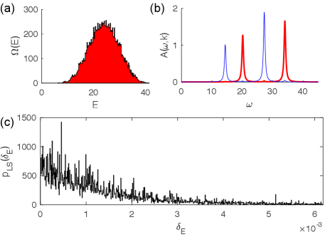
Fig. 2(a) and (c) shows the many-body density of states (DOS) and LSS of the free fermion case () in the sector of total momentum . The other parameters are listed in the caption of Fig. 2, which are chosen sufficiently arbitrary so that there are no additional global symmetries. As one can easily see, the LSS shows a Poisson statistics, due to the many-body integrable nature of free fermions.
Fig. 2(b) shows the zero-temperature spectral weights of (red thick line) and (blue thin line) at momentum , which are defined in Eq. (32). As expected, they show delta function peaks at the single-particle energies of the free chiral Majorana fermions (eigenvalues of Eq. (22)).
The free boson case. As shown in Sec. III.2, when , , and , while the interaction , the model has a global symmetry U(1)U(1)↓, and is solvable as two flavors of free chiral bosons. The conserved symmetry charges are therefore and .
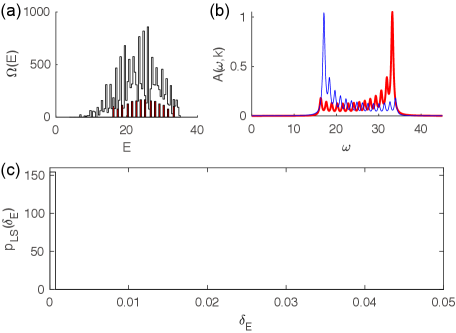
Fig. 3 shows the ED results of such a free-boson example (parameters given in the caption). In Fig. 3(a), the unfilled line is the total DOS of the total momentum sector; while the line filled with red color is the DOS of the finer symmetry sector with quantum numbers . Fig. 3(c) shows the LSS of this symmetry sector , which is almost a delta function at zero. This is because the free bosons’ linear dispersion leads to a large number of many-body level degeneracy. Nonetheless, the LSS can be viewed as a Poisson distribution with a large slope (i.e., small in Eq. (30)).
Fig. 3(b) shows the spectral weights of the spin up (red thick line) and down (blue thin line) fermions in this free boson case, respectively. Analytically, by refermionization, one can derive the spectal weights of the spin fermion as lian2019 ; hu2021chiral ; hu2021integrability (up to energy shifts induced by the chemical potentials and )
| (34) |
where are the coefficients in Eq. (27). This agrees well with the numerical results in Fig. 3(b).
IV.3 The case with U(1) symmetry
We now consider the case of adding a nonzero hopping to the solvable free-boson point, namely,
| (35) |
Due to the nonzero term , the model only has a global U(1) symmetry. Thus, the conserved symmetry charges are the total fermion charge and the total momentum .
In addition, in the special case when , the model Hamiltonian obeys a simple transformation under the particle-hole transformation that flips the U(1) fermion charge :
| (36) |
where for (corresponding to ). In this case (namely, ), the charge sector will have an additional symmetry and thus an additional conserved charge, the eigenvalue of operator . The sectors do not have this additional conserved charge.
Although the model takes a simple form, it cannot be solved as free bosons or free fermions. In the fermion representation, the interaction makes it not free. In the bosonized representation, the term is bosonized into a nonlinear term
| (37) |
making the bosons not free, either. It is not yet known if the model is exactly solvable by certain many-body techniques. Therefore, instead, we examine the ED results of the model in this case.
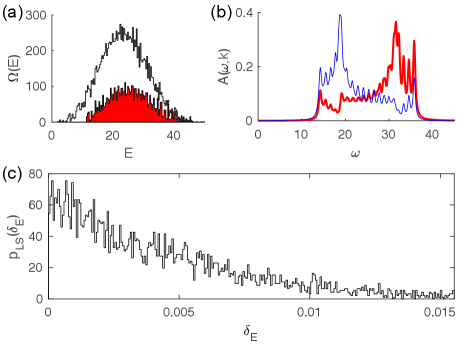
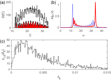
Fig. 4 shows the numerical results for a set of arbitrarily chosen parameters (given in Fig. 4 caption) in this case. Panel (a) shows the DOS of the sector (the unfilled line), and its subsector with symmetry charges with (line filled with red color), which is much smoother compared to the free boson case (Fig. 3(a)). The fermion spectral weights in Fig. 4(b) show irregular shapes, which is an indication of the absence of free fermion or free boson picture.
Intriguingly, the LSS in the finest symmetry sector in this case still shows Poisson statistics among the parameter space we have explored. Fig. 4(c) shows the LSS in the symmetry sector of (i.e., the red part of DOS in Fig. 4(a)). We have examined the LSS in different symmetry sectors for more sets of parameters satisfying Eq. (35), all of which show no level repulsions. This indicates the existence of hidden (quasi)local conserved quantities lian2022conserv beyond those of the global symmetries, which has not been theoretically understood yet. Moreover, the model in this case may be even totally quantum integrable, which we leave for the future studies.
Another similar case with different symmetries will be presented in Sec. IV.4 below. Lastly, we note that when we set in this case, the model will become free fermions with nonlinear dispersions (due to the nonzero ). However, the behavior of the LSS with here (Poisson) is completely different from that of generic nonlinear dispersion fermions with interaction (which is Wigner-Dyson, see Sec. V).
IV.4 The case with U(1) symmetry
In this subsection, we investigate the case with a superconducting pairing: starting from the free boson case with global symmetry U(1)U(1)↓, we turn on the pairing within the spin down flavor, reducing the global symmetry into U(1). The parameters thus satisfy
| (38) |
Accordingly, the conserved charges are and . The parity is dependent on and , as we showed in Eq. (29).
A special case within the parameter space of Eq. (38) is when , for which the model transforms simply under a particle-hole transformation :
| (39) |
Accordingly, when , the charge sector has an additional symmetry , and thus gains an additional conserved charge, the eigenvalue of the operator . This additional charge does not exist in all the sectors.
Such a U(1) symmetry constraint may seem unphysical, that different spins have different symmetries. However, if one regard the spin solely as a fermion flavor index, the model can have its physical context. For instance, it is shown in Ref. hu2021integrability that the interacting chiral edge states of the filling FQH state are equivalent to the interacting fermion model with U(1) here, where the spin fermion carries an irrational electric charge , while the spin fermion is charge neutral. Thus, with charge conservation, pairing is allowed for spin fermions, but not allowed for spin fermions.
With the pairing term , the model has a nonlinear term
| (40) |
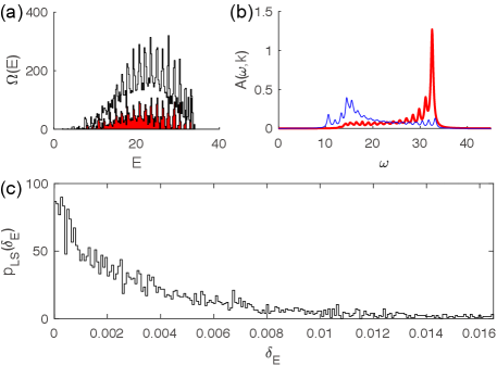
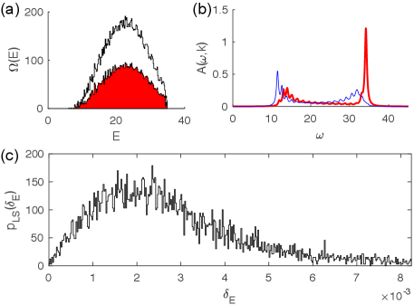
in the bosonized representation. Therefore, the model is neither a free fermion nor a free boson model. Intriguingly, as studied in Ref. hu2021integrability , this model with U(1) symmetry, i.e., with parameters satisfying Eq. (38), shows Poisson LSS in each global symmetry charge sector. Fig. 5 shows the ED results of an example, with the parameters as given in the Fig. 5 caption. The unfilled line and red-filled line in Fig. 5(a) are the DOS of the entire sector and the DOS of the subsector with , respectively. As expected, the fermion spectral weights in Fig. 5(b) are different from those in the free fermion or free boson cases. Fig. 5(c) shows the LSS in the symmetry sector , which is a clear Poisson distribution. More symmetry sectors are examined in Ref. hu2021integrability , all of which shows a Poisson LSS.
Therefore, similar to the U(1) symmetry case we discussed in Sec. IV.3, the Poisson distribution indicates the existence of hidden (quasi)local conserved quantities lian2022conserv , and moreover, the model may be fully quantum integrable. Identifying such hidden conserved quantities is an interesting task for the future studies.
We comment on an observation, that in both the U(1) symmetric case in Sec. IV.3 and the U(1) case here, the bosonized representation of the model has only one nonlinear sine or cosine term in the boson fields : the term in the former case, and the term in the later case. This may be intrinsically related to their Poisson LSS and potential quantum integrability. As we will see in the next few subsections, if one has two or more nonlinear sine or cosine terms, the LSS in each symmetry sector will show Wigner-Dyson statistics.
IV.5 The case with symmetry
We now turn on more pairing terms in our model, and examine its many-body LSS. In this subsection, we consider parameters satisfying
| (41) |
where both spin up and spin down have a nonzero p-wave pairing . It is straightforward to see that each spin has a fermion parity symmetry , with conserved charges , respectively. Moreover, the fact that all the mass terms , are zero leads to another implicit parity symmetry, which we call . The parity charge of this is most easily seen in terms of the Majorana basis defined in Eq. (9), which reads
| (42) |
Similarly, the above three parities and the total momentum are not independent, as Eq. (29) implies. Therefore, a complete set of independent symmetry charges is , and .
In the bosonized representation, the model now has two nonlinear sine or cosine terms given by and :
| (43) |
Therefore, the model is more “nonlinear” compared to the cases in Secs. IV.3 and IV.4.
As shown in Fig. 6, the LSS (Fig. 6(c)) in a fixed symmetry sector (the red part of DOS in Fig. 6(a)) in this case becomes (GOE) Wigner-Dyson statistics. Therefore, we conclude the model in this case is quantum chaotic. The linear ramp at small indicates it resembles a GOE distribution (with in Eq. (31)). Indeed, the Hamiltonian of the model in this case is a real matrix in the momentum space, as protected by a an anti-unitary PT symmetry, where is the spatial inversion and is the spinless time-reversal. Intriguingly, the spectral weights of the model in this case (Fig. 6(b)) is close to that of the free-boson case, despite being a quantum chaotic model.
IV.6 The case with symmetry
The global symmetry of the model can be further lowered down to only if the parameters satisfy
| (44) |
Compared to the case in Eq. (41), here the presence of nonzero or breaks the conservation of the parity charge in Eq. (42). Therefore, the independent symmetry charges in this case are and .
The ED results for this case is shown in Fig. 7. Fig. 7(a) shows the DOS of the total sector of momentum and the symmetry subsector with . The LSS of this symmetry subsector is given in Fig. 7(c), which shows a GOE (linear at small ) Wigner-Dyson shape. Therefore, similar to the case in Sec. IV.5, the model here with symmetry is also quantum chaotic. The GOE distribution is also due to the presence of a PT symmetry, which restricts the Hamiltonian in the momentum space to be real. The spectral weights show clear deviations from that in the free-boson case.
IV.7 The case with symmetry
In the last case, if we do not impose any constraints on the parameters, the model only has a global fermion parity symmetry, the symmetry charge of which is (Eq. (29)). Therefore, the only independent conserved charge is .
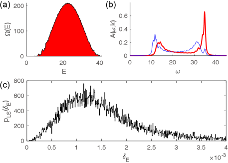
Fig. 8 shows a ED calculation for parameters (see the caption) in this generic case. In the symmetry sector of total momentum , the DOS distribution (Fig. 8(a)) is much smoother than all the higher symmetry cases we discussed earlier. The fermion spectral weights in Fig. 8(b) also shows less discretized peaks., indicating a higher randomness in the energy spectrum. Fig. 8(c) shows the LSS of the sector, which is quadratic at small , and thus resembles the GUE Wigner-Dyson distribution (namely, in Eq. (31)). This is because, with the parameters and being generically complex, the model does not have a PT symmetry or other anti-unitary symmetry, and the Hamiltonian is generically in the complex class. Therefore, one expects a GUE LSS in each symmetry charge sector. The model with only a symmetry is therefore many-body quantum chaotic.
V The effect of nonlinear dispersion
It is worthwhile to compare the numerical results of our model in the above cases in Sec. IV with the interacting model with a nonlinear dispersion added. To be explicit, we start with the free-boson solvable point, namely, the Hamiltonian in Eq. (5) with parameters satisfying Eq. (23) (which has U(1)U(1)(↓) symmetry), and add a cubic dispersion term
| (45) |
where is the the coupling strength. This yields a free-fermion dispersion . Such nonlinear terms are irrelevant, so one expects it not to affect the low energy physics. This term does not affect the global symmetry of the model. However, this nonlinear term will break the quantum integrability of the model (at energy scales where this term cannot be ignored).
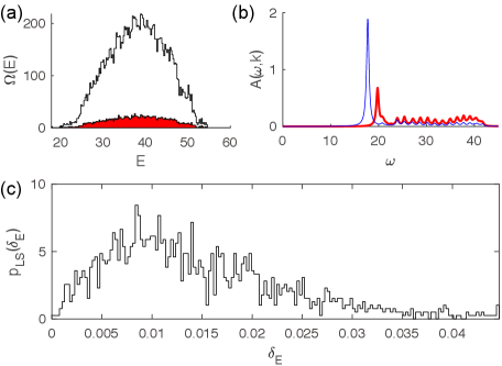
Fig. 9 shows the ED results for such a model with a large nonlinear dispersion (the other parameters given in the caption). Compared with the linear dispersion case in Fig. 3, the nonlinear term makes the DOS much smoother (Fig. 9(a)), distorts the fermion spectral weights (Fig. 9(b)), and changes the LSS in each symmetry charge sector into a GOE Wigner-Dyson distribution. Therefore, the model shows quantum chaos due to the nonlinear dispersion term.
An intriguing case which can be compared with the current case is the U(1) symmetric case we studied in Sec. IV.3, which has a generic nonzero matrix. Diagonalizing the free fermion part of the U(1) symmetric case Hamiltonian (i.e., Eq. (22)) yields a nonlinear fermion dispersion in the eigen-fermion basis. Therefore, it is also an interacting fermion problem with nonlinear dispersions. However, in the U(1) symmetric case, each of the symmetry charge sector shows Poisson LSS, which is drastically different from the nonlinear model in this section. Therefore, the U(1) symmetric case in Sec. IV.3 is a special nonlinear dispersion model with hidden conserved quantities.
VI Discussion
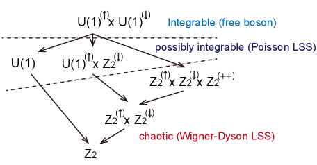
We have demonstrated that a simple interacting model of two-flavors of chiral fermions shows a rich transition of quantum integrability/chaos with respect to the global symmetries of the model. In the model, we have ignored all the irrelevant terms (except for Sec. V), the effects of which will be suppressed at low energies. Starting from the solvable Luttinger liquid point which yields free chiral bosons with linear dispersions, the lowering of global symmetries leads to a transition to possibly integrable (Poisson LSS in each symmetry sector) energy spectrum and then to quantum chaotic (Wigner-Dyson LSS in each symmetry sector) energy spectrum. Fig. 10 summarizes this integrable to chaotic transition process versus the global symmetries (the translation symmetry is not listed, which is always there). In particular, the Poisson LSS (possibly integrable) regime indicates there exist hidden (quasi)local conserved quantities, and it would be interesting and useful to explore what they are. It would also be helpful to explore the transition behavior from Poisson to Wigner-Dyson LSS vir2021 due to symmetry breaking. Numerically, one possible method is to detect such conserved quantities from their eigenstate reduced density matrices (entanglement Hamiltonians) lian2022conserv .
One future question is how the integrable or chaotic energy spectra affect the low-energy quantum dynamics of the excitations in such 1D chiral systems, which may be realized as the edge states of 2D topological phases. For the cases with Poisson LSS in each global symmetry sector, the hidden conserved quantities could protect (fully or partially) the quantum coherence of the edge states in certain ways, which may be detectable in edge state interferometer experiments, such as the Fabry-Pérot interferometer geometry Nakamura2020 and tunnel junctions Lian2016 ; Lian2018a ; Fu2009 ; Akhmerov2009 . In particular, it is possible to control the global symmetries of the chiral edge states experimentally to examine the differences in quantum dynamics with respect to symmetries (Fig. 10). For instance, by adding superconducting proximity, one may reduce the symmetry of the model from U(1) to . Besides, Ref. hu2021integrability shows that the model in the U(1) symmetry case is equivalent to the interacting chiral edge states of the 4/3 FQH state and a class of other bilayer FQH states.
The present model can be further generalized into fractionalized anyonic models. such as the FQH edge states hu2021integrability ; naud2000 and Wess-Zumino-Witten (WZW) models wess1971 ; witten1983 ; novikov1982 ; witten1984 ; hu2021chiral . An example of large number of interacting WZW models is studied in Ref. hu2021chiral . Moreover, the effect of spatial disorders on the quantum integrability are yet to be investigated, which, however, will break the translational symmetry and makes the ED numerical calculations extremely difficult. Thus, new methods are desired for studying such systems.
Acknowledgements.
Acknowledgments. The author is honored to contribute to the Chen-Ning Yang Centenary Festschrift. This work is supported by the Alfred P. Sloan Foundation, and NSF through the Princeton University’s Materials Research Science and Engineering Center DMR-2011750.References
- [1] H. Bethe. Zur theorie der metalle i. eigenwerte und eigenfunktionen der linearen atomkette. Z. Phys., 71:205, 1931.
- [2] Lars Onsager. Crystal statistics. i. a two-dimensional model with an order-disorder transition. Phys. Rev., 65:117–149, Feb 1944.
- [3] Elliott H. Lieb and Werner Liniger. Exact analysis of an interacting bose gas. i. the general solution and the ground state. Phys. Rev., 130:1605–1616, May 1963.
- [4] Elliott H. Lieb. Exact analysis of an interacting bose gas. ii. the excitation spectrum. Phys. Rev., 130:1616–1624, May 1963.
- [5] Elliott H. Lieb and F. Y. Wu. Absence of mott transition in an exact solution of the short-range, one-band model in one dimension. Phys. Rev. Lett., 20:1445–1448, Jun 1968.
- [6] J. B. McGuire. Study of exactly soluble one‐dimensional n‐body problems. Journal of Mathematical Physics, 5(5):622–636, 1964.
- [7] C. N. Yang. Some exact results for the many-body problem in one dimension with repulsive delta-function interaction. Phys. Rev. Lett., 19:1312–1315, Dec 1967.
- [8] R. J. Baxter. Eight-vertex model in lattice statistics. Phys. Rev. Lett., 26:832–833, Apr 1971.
- [9] I. E. DzyaloshinskiĬ and A. I. Larkin. Correlation functions for a one-dimensional fermi system with long-range interaction (tomonaga model). In 30 Years of the Landau Institute — Selected Papers, pages 95–101. WORLD SCIENTIFIC, August 1996.
- [10] F D M Haldane. ‘luttinger liquid theory’ of one-dimensional quantum fluids. i. properties of the luttinger model and their extension to the general 1d interacting spinless fermi gas. Journal of Physics C: Solid State Physics, 14(19):2585–2609, jul 1981.
- [11] F. D. M. Haldane. Effective harmonic-fluid approach to low-energy properties of one-dimensional quantum fluids. Phys. Rev. Lett., 47:1840–1843, Dec 1981.
- [12] S. i. Tomonaga. Remarks on bloch’s method of sound waves applied to many-fermion problems. Progress of Theoretical Physics, 5(4):544–569, July 1950.
- [13] J. M. Luttinger. An exactly soluble model of a many-fermion system. Journal of Mathematical Physics, 4(9):1154–1162, September 1963.
- [14] X. G. Wen. Chiral luttinger liquid and the edge excitations in the fractional quantum hall states. Phys. Rev. B, 41:12838–12844, Jun 1990.
- [15] X. G. Wen. Gapless boundary excitations in the quantum hall states and in the chiral spin states. Phys. Rev. B, 43:11025–11036, May 1991.
- [16] C. N. Yang. The spontaneous magnetization of a two-dimensional ising model. Phys. Rev., 85:808–816, Mar 1952.
- [17] C. N. Yang and C. P. Yang. Ground-state energy of a heisenberg-ising lattice. Phys. Rev., 147:303–306, Jul 1966.
- [18] C. N. Yang and C. P. Yang. One-dimensional chain of anisotropic spin-spin interactions. i. proof of bethe’s hypothesis for ground state in a finite system. Phys. Rev., 150:321–327, Oct 1966.
- [19] C. N. Yang and C. P. Yang. One-dimensional chain of anisotropic spin-spin interactions. ii. properties of the ground-state energy per lattice site for an infinite system. Phys. Rev., 150:327–339, Oct 1966.
- [20] C. N. Yang and C. P. Yang. One-dimensional chain of anisotropic spin-spin interactions. iii. applications. Phys. Rev., 151:258–264, Nov 1966.
- [21] C. N. Yang and C. P. Yang. Thermodynamics of a one‐dimensional system of bosons with repulsive delta‐function interaction. Journal of Mathematical Physics, 10(7):1115–1122, 1969.
- [22] Marcos Rigol, Vanja Dunjko, Vladimir Yurovsky, and Maxim Olshanii. Relaxation in a completely integrable many-body quantum system: An ab initio study of the dynamics of the highly excited states of 1d lattice hard-core bosons. Phys. Rev. Lett., 98:050405, Feb 2007.
- [23] Marcos Rigol, Vanja Dunjko, and Maxim Olshanii. Thermalization and its mechanism for generic isolated quantum systems. Nature, 452(7189):854–858, Apr 2008.
- [24] M. G. Tetelman. Lorentz group for two-dimensional integrable lattice systems. Sov. Phys. JETP, 55:306, 1981.
- [25] M.P. Grabowski and P. Mathieu. Structure of the conservation laws in quantum integrable spin chains with short range interactions. Annals of Physics, 243(2):299–371, 1995.
- [26] Enej Ilievski, Marko Medenjak, and Toma ž Prosen. Quasilocal conserved operators in the isotropic heisenberg spin- chain. Phys. Rev. Lett., 115:120601, Sep 2015.
- [27] Yuji Nozawa and Kouhei Fukai. Explicit construction of local conserved quantities in the spin- chain. Phys. Rev. Lett., 125:090602, Aug 2020.
- [28] Biao Lian. Conserved quantities from entanglement hamiltonian. Phys. Rev. B, 105:035106, Jan 2022.
- [29] Subir Sachdev and Jinwu Ye. Gapless spin fluid ground state in a random, quantum Heisenberg magnet. Phys. Rev. Lett., 70:3339, 1993.
- [30] Joseph Polchinski and Vladimir Rosenhaus. The Spectrum in the Sachdev-Ye-Kitaev Model. JHEP, 04:001, 2016.
- [31] Juan Maldacena and Douglas Stanford. Remarks on the Sachdev-Ye-Kitaev model. Phys. Rev., D94(10):106002, 2016.
- [32] Alexei Kitaev and S. Josephine Suh. The soft mode in the Sachdev-Ye-Kitaev model and its gravity dual. JHEP, 05:183, 2018.
- [33] Biao Lian, S. L. Sondhi, and Zhenbin Yang. The chiral SYK model. Journal of High Energy Physics, 2019(9), September 2019.
- [34] Yichen Hu and Biao Lian. The Chiral Sachdev-Ye Model: Integrability and Chaos of Anyons in 1+1d. arXiv e-prints, page arXiv:2109.13263, September 2021.
- [35] Juan Maldacena, Stephen H. Shenker, and Douglas Stanford. A bound on chaos. JHEP, 08:106, 2016.
- [36] O. Bohigas, M. J. Giannoni, and C. Schmit. Characterization of chaotic quantum spectra and universality of level fluctuation laws. Phys. Rev. Lett., 52:1–4, Jan 1984.
- [37] Freeman J. Dyson. Correlations between eigenvalues of a random matrix. Communications in Mathematical Physics, 19(3):235–250, September 1970.
- [38] Eugene P. Wigner. Random matrices in physics. SIAM Review, 9(1):1–23, January 1967.
- [39] R. V. Jensen and R. Shankar. Statistical behavior in deterministic quantum systems with few degrees of freedom. Phys. Rev. Lett., 54:1879–1882, Apr 1985.
- [40] J. M. Deutsch. Quantum statistical mechanics in a closed system. Phys. Rev. A, 43:2046–2049, Feb 1991.
- [41] Mark Srednicki. Chaos and quantum thermalization. Phys. Rev. E, 50:888–901, Aug 1994.
- [42] Luca D’Alessio, Yariv Kafri, Anatoli Polkovnikov, and Marcos Rigol. From quantum chaos and eigenstate thermalization to statistical mechanics and thermodynamics. Advances in Physics, 65(3):239–362, 2016.
- [43] M. V. Berry and M. Tabor. Level clustering in the regular spectrum. Proceedings of the Royal Society of London. A. Mathematical and Physical Sciences, 356(1686):375–394, September 1977.
- [44] Gregory Moore and Nicholas Read. Nonabelions in the fractional quantum hall effect. Nucl. Phys. B, 360(2):362 – 396, 1991.
- [45] X. G. Wen. Non-abelian statistics in the fractional quantum hall states. Phys. Rev. Lett., 66:802–805, Feb 1991.
- [46] F. D. M. Haldane. Stability of chiral luttinger liquids and abelian quantum hall states. Phys. Rev. Lett., 74:2090–2093, Mar 1995.
- [47] C. L. Kane, Matthew P. A. Fisher, and J. Polchinski. Randomness at the edge: Theory of quantum hall transport at filling . Phys. Rev. Lett., 72:4129–4132, Jun 1994.
- [48] Michael Levin, Bertrand I. Halperin, and Bernd Rosenow. Particle-hole symmetry and the pfaffian state. Phys. Rev. Lett., 99:236806, Dec 2007.
- [49] Sung-Sik Lee, Shinsei Ryu, Chetan Nayak, and Matthew P. A. Fisher. Particle-hole symmetry and the quantum hall state. Phys. Rev. Lett., 99:236807, Dec 2007.
- [50] Michael Levin. Protected edge modes without symmetry. Phys. Rev. X, 3:021009, May 2013.
- [51] Juven C. Wang and Xiao-Gang Wen. Boundary degeneracy of topological order. Phys. Rev. B, 91:125124, Mar 2015.
- [52] Biao Lian and Juven Wang. Theory of the disordered quantum thermal hall state: Emergent symmetry and phase diagram. Phys. Rev. B, 97:165124, Apr 2018.
- [53] C. de C. Chamon and X. G. Wen. Sharp and smooth boundaries of quantum hall liquids. Phys. Rev. B, 49:8227–8241, Mar 1994.
- [54] Xin Wan, Kun Yang, and E. H. Rezayi. Reconstruction of fractional quantum hall edges. Phys. Rev. Lett., 88:056802, Jan 2002.
- [55] Xin Wan, E. H. Rezayi, and Kun Yang. Edge reconstruction in the fractional quantum hall regime. Phys. Rev. B, 68:125307, Sep 2003.
- [56] Ron Sabo, Itamar Gurman, Amir Rosenblatt, Fabien Lafont, Daniel Banitt, Jinhong Park, Moty Heiblum, Yuval Gefen, Vladimir Umansky, and Diana Mahalu. Edge reconstruction in fractional quantum hall states. Nature Physics, 13(5):491–496, January 2017.
- [57] Jennifer Cano, Meng Cheng, Michael Mulligan, Chetan Nayak, Eugeniu Plamadeala, and Jon Yard. Bulk-edge correspondence in (2 + 1)-dimensional abelian topological phases. Phys. Rev. B, 89:115116, Mar 2014.
- [58] Yichen Hu and Biao Lian. Integrability of the fractional quantum hall edge states, 2021.
- [59] Frank Schindler, Nicolas Regnault, and B. Andrei Bernevig. Exact Quantum Scars in the Chiral Non-Linear Luttinger Liquid. arXiv e-prints, page arXiv:2110.15365, October 2021.
- [60] I. Martin and K. A. Matveev. Scar states in a system of interacting chiral fermions. arXiv e-prints, page arXiv:2109.06220, September 2021.
- [61] R. L. Willett, L. N. Pfeiffer, and K. W. West. Measurement of filling factor 5/2 quasiparticle interference with observation of charge e/4 and e/2 period oscillations. Proceedings of the National Academy of Sciences, 106(22):8853–8858, May 2009.
- [62] Lingfei Zhao, Ethan G. Arnault, Alexey Bondarev, Andrew Seredinski, Trevyn F. Q. Larson, Anne W. Draelos, Hengming Li, Kenji Watanabe, Takashi Taniguchi, François Amet, Harold U. Baranger, and Gleb Finkelstein. Interference of chiral andreev edge states. Nature Physics, 16(8):862–867, May 2020.
- [63] Biao Lian, Jing Wang, and Shou-Cheng Zhang. Edge-state-induced andreev oscillation in quantum anomalous hall insulator-superconductor junctions. Phys. Rev. B, 93:161401, Apr 2016.
- [64] Preden Roulleau, F. Portier, P. Roche, A. Cavanna, G. Faini, U. Gennser, and D. Mailly. Direct measurement of the coherence length of edge states in the integer quantum hall regime. Phys. Rev. Lett., 100:126802, Mar 2008.
- [65] R. B. Laughlin. Anomalous quantum hall effect: An incompressible quantum fluid with fractionally charged excitations. Phys. Rev. Lett., 50:1395–1398, May 1983.
- [66] J. Nakamura, S. Liang, G. C. Gardner, and M. J. Manfra. Direct observation of anyonic braiding statistics. Nature Physics, 16(9):931–936, September 2020.
- [67] Matteo Carrega, Luca Chirolli, Stefan Heun, and Lucia Sorba. Anyons in quantum hall interferometry. Nature Reviews Physics, September 2021.
- [68] D. T. McClure, W. Chang, C. M. Marcus, L. N. Pfeiffer, and K. W. West. Fabry-perot interferometry with fractional charges. Phys. Rev. Lett., 108:256804, Jun 2012.
- [69] N. Ofek, A. Bid, M. Heiblum, A. Stern, V. Umansky, and D. Mahalu. Role of interactions in an electronic fabry-perot interferometer operating in the quantum hall effect regime. Proceedings of the National Academy of Sciences, 107(12):5276–5281, March 2010.
- [70] Bertrand I. Halperin, Ady Stern, Izhar Neder, and Bernd Rosenow. Theory of the fabry-pérot quantum hall interferometer. Phys. Rev. B, 83:155440, Apr 2011.
- [71] Mitali Banerjee, Moty Heiblum, Vladimir Umansky, Dima E. Feldman, Yuval Oreg, and Ady Stern. Observation of half-integer thermal hall conductance. Nature, 559(7713):205–210, June 2018.
- [72] D. E. Feldman. Comment on “interpretation of thermal conductance of the edge”. Phys. Rev. B, 98:167401, Oct 2018.
- [73] Steven H. Simon. Interpretation of thermal conductance of the edge. Phys. Rev. B, 97:121406, Mar 2018.
- [74] Ken K. W. Ma and D. E. Feldman. Partial equilibration of integer and fractional edge channels in the thermal quantum hall effect. Phys. Rev. B, 99:085309, Feb 2019.
- [75] Vir B. Bulchandani, David A. Huse, and Sarang Gopalakrishnan. Onset of many-body quantum chaos due to breaking integrability. arXiv e-prints, page arXiv:2112.14762, December 2021.
- [76] Biao Lian, Xiao-Qi Sun, Abolhassan Vaezi, Xiao-Liang Qi, and Shou-Cheng Zhang. Topological quantum computation based on chiral majorana fermions. Proceedings of the National Academy of Sciences, 115(43):10938–10942, October 2018.
- [77] Liang Fu and C. L. Kane. Probing neutral majorana fermion edge modes with charge transport. Phys. Rev. Lett., 102:216403, May 2009.
- [78] A. R. Akhmerov, Johan Nilsson, and C. W. J. Beenakker. Electrically detected interferometry of majorana fermions in a topological insulator. Phys. Rev. Lett., 102:216404, May 2009.
- [79] J. D. Naud, Leonid P. Pryadko, and S. L. Sondhi. Quantum Hall bilayers and the chiral sine-Gordon equation. Nuclear Physics B, 565(3):572–610, February 2000.
- [80] J. Wess and B. Zumino. Consequences of anomalous ward identities. Physics Letters B, 37(1):95–97, 1971.
- [81] Edward Witten. Global aspects of current algebra. Nuclear Physics B, 223(2):422–432, 1983.
- [82] S. P. Novikov. The Hamiltonian formalism and a many valued analog of Morse theory. Usp. Mat. Nauk, 37N5(5):3–49, 1982.
- [83] Edward Witten. Nonabelian Bosonization in Two-Dimensions. Commun. Math. Phys., 92:455–472, 1984.