Intelligent Reflecting Surface Configurations for Smart Radio Using Deep Reinforcement Learning
Abstract
Intelligent reflecting surface (IRS) is envisioned to change the paradigm of wireless communications from “adapting to wireless channels” to “changing wireless channels”. However, current IRS configuration schemes, consisting of sub-channel estimation and passive beamforming in sequence, conform to the conventional model-based design philosophies and are difficult to be realized practically in the complex radio environment. To create the smart radio environment, we propose a model-free design of IRS control that is independent of the sub-channel channel state information (CSI) and requires the minimum interaction between IRS and the wireless communication system. We firstly model the control of IRS as a Markov decision process (MDP) and apply deep reinforcement learning (DRL) to perform real-time coarse phase control of IRS. Then, we apply extremum seeking control (ESC) as the fine phase control of IRS. Finally, by updating the frame structure, we integrate DRL and ESC in the model-free control of IRS to improve its adaptivity to different channel dynamics. Numerical results show the superiority of our proposed joint DRL and ESC scheme and verify its effectiveness in model-free IRS control without sub-channel CSI.
I Introduction
Metasurfaces, which consist of artificially periodic or quasi-periodic structures with sub-wavelength scales, are a new design of functional materials [1, 2]. Some extraordinary electromagnetic properties observed on metasurfaces, e.g., negative permittivity and permeability, reveal its potential in tailoring electromagnetic waves in a wide frequency range, from microwave to visible light [3, 4, 5, 6]. Intelligent reflecting surface (IRS), a.k.a. reconfigurable intelligent surface (RIS), is a type of programmable metasurfaces that is capable of electronically tuning electromagnetic wave by incorporating active components into each unit cell of metasurfaces [7, 8, 9, 10, 11, 12]. The advent of IRS is envisioned to revolutionize many industries, a major one of which is wireless communications.
Wireless communications are subject to the time-varying radio propagation environment. The effects of free space path loss, signal absorption, reflections, refractions, and diffractions caused by physical objects during the propagation of electromagnetic waves jointly render wireless channels highly dynamic [13, 14, 15]. IRS’s capability of manipulating electromagnetic waves in a real time manner brings infinite possibilities to wireless communications and makes it possible for human beings to transform the design paradigm of wireless communications from “adapting to wireless channels” to “changing wireless channels” [7]. To this end, great research efforts have been spent to acquire the channel state information (CSI) of the sub-channels, i.e., the channels between wireless transceivers and IRS, which is widely regarded as the prerequisite of IRS reflection pattern (passive beamforming) design [8]. Owing to the passive nature, IRS is unable to sense the incident signal, thereby rendering the estimation process far more complicated than traditional wireless communication systems. In [9], a channel estimation scheme with reduced training overhead is proposed by exploiting the inter-user channel correlation. In [10, 11], compressed sensing based channel estimation methods are proposed to estimate the channel responses between base station, IRS and a single-antenna user at mmWave frequency band. As the proposed schemes are focusing on a single-antenna user, their extension to multiple users with array antenna might increase multi-fold the training overhead. In [16], a joint beam training and positioning scheme is proposed to estimate the parameters of the line-of-sight (LoS) paths for IRS assisted mmWave communications. The proposed random beamforming in the training stage is performed in a broadcasting manner and thus the training overhead is independent of the user number.
Despite the aforementioned endeavors to advance the CSI acquisition techniques in IRS assisted wireless communications, the practical applications of IRS are still confronting various challenges. Firstly, channel estimations for IRS assisted wireless communications demand a radical update of the existed protocols to incorporate the coordination of the transmitter, the receiver, and the IRS. It indicates that the existing wireless systems, e.g., Wi-Fi, 4G-LTE and 5G-NR, are unable to readily embrace IRS. Secondly, even if the perfect CSI is available, the real-time optimization of IRS reflection coefficients using convex and non-convex optimization techniques is computationally prohibitive [12]. Thirdly, current solutions to IRS control, which consists of CSI acquisition and IRS reflection designs, are based on the accurate modelling of IRS. However, as a type of low-cost reflective metasurfaces, IRS changes its reflection coefficient via tuning the impedance, the exact value of which is dependant on the carrier frequency of the incident signal [17, 18]. The carrier frequency can be shifted by Doppler effects and might also vary over different users, thus the mathematical modelling of IRS in the complex radio propagation environment is inherently difficult.
To tackle the aforementioned challenges, we follow the design paradigm of model-free control by treating the wireless communication system as a (semi) black box with uncertain parameters and to optimize reflection coefficients of IRS through deep reinforcement learning (DRL) and extremum seeking control (ESC). Compared with the prevailing designs of IRS assisted wireless communication systems [11, 19, 20, 21, 22, 23, 24, 25, 26], our proposed scheme is model-free. Specifically, the instantaneous (or statistical) CSI of sub-channels (i.e., Tx-Rx channel, Tx-IRS channel, and IRS-Rx channel) that constitutes the equivalent wireless channel is not required. Our design, in a true sense, treats IRS as a part of the wireless channel and requires the minimum interaction with wireless communication systems. The disentanglement of IRS configuration from wireless communication system means the improved independence of IRS and will speed up the rollout of IRS in the future. There are already some attempts towards the standalone operation of IRS [27, 28, 29]. In [27, 28], deep learning and deep reinforcement learning are applied to guide the IRS to interact with the incident signal given the knowledge of the sampled channel vectors. However, in order to obtain the CSI of the Tx-IRS and IRS-Rx sub-channels, the authors propose to install channel sensors on the IRS, which is, to some extent, against the initial role of IRS as a passive device. In [29], to reduce the dependance on the CSI of sub-channels, a deep learning scheme is proposed to extract the interactions between phase shifts of IRS and receiver locations. However, the training data has to be collected offline, which limits its adaptability to the more general scenarios.
In this paper, our objective is to build a model-free IRS control scheme with a higher level understanding of the radio environment, which is able to configure the IRS reflection coefficients without the CSI of the sub-channels. To this end, we adopt a typical scenario, i.e., time-division duplexing (TDD) multi-user multiple-input-multiple-output (MIMO), as an example to perform our design. To summarize, our contributions are as follows.
-
•
We model the control of IRS as a Markov decision process (MDP) and then apply DRL, specifically, double deep Q-network (DDQN) method, to perform real-time coarse phase control of IRS. The proposed DDQN scheme outperforms the other sub-channel-CSI-independent methods, e.g., multi-armed bandit (MAB), random reflection.
-
•
To enhance the action of DDQN, we further apply ESC as the fine phase control of IRS. Specifically, we propose a dither-based iterative method to optimize the phase shift of IRS through trial and error. We also prove that the output of the proposed dither-based iterative method is monotonically increasing.
-
•
By updating the frame structure, we integrate DRL and ESC in the model-free control of IRS. The integrated scheme is more adaptive to various channel dynamics and has the potential to achieve better performance.
Numerical results show the superiority of our proposed DRL, ESC, and joint DRL and ESC scheme and verify their effectiveness in model-free IRS control without sub-channel CSI.
The rest of the paper is organized as follows. In Section II, we introduce the system model. In Section III, we propose a DRL enabled model-free control of IRS. In Section IV, we propose a dither-based iterative method to enhance the action of DRL. In Section V, we present numerical results. Finally, in Section VII, we draw the conclusion.
Notations: Column vectors (matrices) are denoted by bold-face lower (upper) case letters, denotes the -th element in the vector , represents the Hadamard product, , and represent conjugate, transpose and conjugate transpose operation, respectively.
II System Model
In this section, we introduce the system model of model-free IRS control.
II-A Optimal Phase Shift Vector of IRS
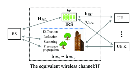
For IRS assisted wireless communications, the channel model between BS and a certain user can be represented as
| (1) |
where the user is equipped with a single antenna, is the channel response vector between the user and BS, is the channel response matrix between BS and IRS, is the channel response vector between the user and IRS, , and (with ) is the phase shift vector of the IRS. Accordingly, the multi-user channel is written as
| (2) |
where
And the relationship between the aggregated equivalent channel and the sub-channels is shown in Figure 1.
The objective of reinforcement learning based IRS configuration is to develop a widely compatible method that can be deployed in various scenarios of wireless communications without any knowledge of the wireless system’s internal working mechanism. Mathematically, the problem is formulated as
| (3) | ||||
where is the performance metric of the wireless system that is to be optimized. is dependent on the wireless channel , and is dependent on the reflection pattern . is the quantized phase selected from a finite set with possible values.
It is worth mentioning that the model-free control does not need to know the exact relationship between the objective and variable .
II-B A Typical Scenario – TDD Multi-User MIMO
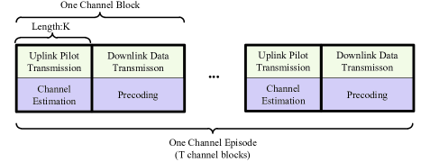
Without loss of generality, we use a typical scenario in wireless communication, i.e., TDD multi-user MIMO, to illustrate our design philosophy. In TDD, by exploiting the channel reciprocity, the BS can estimate the downlink channel from the pilot of the uplink channel. Thus, TDD multi-user MIMO consists of two stages (refer to Figure 2), i.e., uplink pilot transmission and downlink data transmission[30, 31].
At uplink stage, the pilot transmits from multiple users to BS simultaneously. The received pilot signal is represented as
| (4) |
where is the pilot pattern, is the additive white Gaussian noise. Upon receiving the pilot, BS performs minimum mean square error (MMSE) estimation of the channel matrix, i.e.,
| (5) |
When is an unitary matrix, (5) is further expressed as
| (6) |
At downlink stage, data transmission with zero-forcing (ZF) precoding is performed, and the precoding matrix is represented as
| (7a) | ||||
| (7b) | ||||
where is for power normalization. The received signal of user is given by
| (8) |
where is the signal intended to user ( and , ), and is the additive white Gaussian noise. Thus, the signal-to-noise ratio of the -th user is
| (9) |
For a communication system, the performance metrics can be SINR, data rate, frame error rate (FER), and etc. Without loss of generality, we adopt the sum data rate as the performance metric, i.e.,
| (10) |
II-C Channel Model
We assume the Rician channel model for , and . Take as an example, it is represented as
| (11) |
where denotes the deterministic LoS component, denotes the fast fading NLoS component, and the component of which is independent and identically distributed (i.i.d.) circularly symmetric complex Gaussian random variables with zero-mean and unit variance, and is the ratio between the power in the LoS path and the power in the NLoS paths [32].
The LoS component is position-dependent and is thus slow-time-varying; The NLoS components are caused by the multi-path effects and are thus fast-time-varying [33]. Combining the characteristics of wireless channel with the setting of reinforcement learning, we introduce the following two concepts.
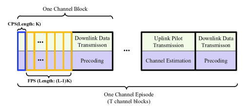
(1) Channel block: One channel block consists of the uplink pilot transmission stage and downlink data transmission stage (as shown in Figure 2), and the channel matrix is constant during the channel block.
(2) Channel episode: One channel episode consists of channel blocks (as shown in Figure 2). The LoS component within one channel episode remains constant; The NLoS components change over time, and the NLoS components of different channel blocks are i.i.d.
III Model-Free IRS Control Enabled By Deep Reinforcement Learning
In this section, we apply DRL to model-free IRS control.
III-A Design Objectives
We aim to achieve stand-alone operation of the wireless communication system and the IRS, and our design includes the following characteristics.
-
•
Wireless Communication System: The wireless communication system is almost unaware of the existence of the IRS, except that it needs to feed back its instantaneous performance to the IRS controller. In this regard, the uplink pilot transmission and downlink data transmission exactly follow the conventional structure in Figure 2.
-
•
IRS: The IRS is strictly regarded as part of the wireless channel and will not be jointly designed with the wireless communication system. The configuration of IRS is based on (a) the performance feedback from the wireless system and (b) its learned policy through trail-and-error interaction with the dynamic environment. And the IRS is unaware of the working mechanism of the wireless communication system.
A salient advantage of the proposed design is that the IRS can be deployed in various wireless communication applications, e.g., Wi-Fi, 4G-LTE, 5G-NR, without updating their existing protocols, which will speed up the roll-out of IRSs. Another benefit is that, by treating the existing wireless communication system as a black box, the configuration of IRS does not require the overhead-demanding channel sounding process to acquire the CSI of the subchannels, i.e., , , and , that constitute the aggregated equivalent channel .
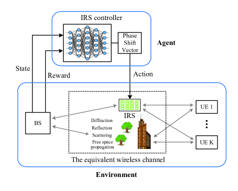
Our design is primarily based on the reinforcement learning technology. Specifically, the IRS and its controller are the agent, the wireless communication system, which comprises transmitter, wireless channel, and receiver, is the environment. The relationship between the different parties is given in Figure 3. Initially, the agent takes random actions and the environment responds to those actions by giving rise to rewards and presenting new situations to the agent [34, 35]. Through trail-and-error interaction with the wireless communication system, the agent gradually learns the optimal policy to maximize the expected return over time. In this regard, IRS, which is capable of changing the radio environment, is analogous to the human body, and the reinforcement learning method, which guides the action of IRS, is analogous to the human brain. The integration of the IRS and the reinforcement learning method is the pathway to creating the smart radio environment.
III-B Basics of Deep Reinforcement Learning
To facilitate the presentation of our design, we briefly introduce some key concepts of DRL in this subsection.
III-B1 Objective of Reinforcement Learning
An MDP is specified by -tuple , where is the state space, is the action space, is the state transition probability, and is the immediate reward received by the agent. When an agent in the state takes the action , the environment will evolve to the next state with probability , and in the meantime, the agent will receive the immediate reward . Adding the time index to , the evolution of an MDP can be represented using the following trajectory
| (12) |
The agent’s action is directed by the policy function
| (13) |
which is the probability that the agent takes action when the current state is . A reinforcement learning task intends to find a policy that achieves a good return over the long run, where the return is defined as the cumulative discounted future reward, i.e.,
and is the discount factor for future rewards. Owing to the randomness of state transition (caused by the dynamic environment) and action selection, the return is a random variable. Mathematically, the agent’s goal in reinforcement learning is to find a good policy that maximizes the expected return, i.e.,
| (14) |
III-B2 Action-Value Function and Optimal Policy
One key metric for action selection in reinforcement learning is action-value function, i.e.,
| (15) |
which is the conditional expected return for an agent to pick action in the state under the policy . For any policy and any state , action-value function satisfies the following recursive relationship, i.e.,
| (16) |
where is the immediate reward when the environment transits from state to state after taking the action , and Eq. (16) is the well-known Bellman equation of action-value function [34].
A policy is defined to be better than another policy if its expected return is greater than that of for all states and all actions. Thus, the optimal action-value function is
| (17) |
With the optimal action-value function, the optimal policy is obviously
| (20) |
Combining (17), (20) with (16), the Bellman optimality equation for is given by
| (21) |
With the Bellman optimality equation, the optimal policy or the optimal action-value function can be obtained via iterative methods, i.e., policy iteration based methods and value iteration based methods[34]. Hereinafter, we will mainly focus on value iteration based methods.
III-B3 Temporal Difference Learning
The aforementioned iterative methods require the complete knowledge of the environment, i.e., state transition probability , reward function , etc. However, the explicit knowledge of environment dynamics is unavailable in practice. The conditional expectation in (21) can be realized via numerically averaging over the sample sequences of states, actions, and rewards from actual interaction with the environment, e.g., temporal difference method, or Monte Carlo method.
Upon observing a new segment of the trajectory in (12), i.e., , the action-value function updates as follows:
| (22) |
where is the learning rate and the following term inside the bracket is the error between the estimated Q value and the return. It means that the value function is updated in the direction of the error, and iteration will terminate when the error becomes infinitesimal.
III-B4 Double Deep Q-Network (DDQN)
When the state and the action are both discrete, the optimal state-action function can be obtained as a lookup table, which is also known as Q-table [36], following the iterative procedures in (22). However, the size of the state (or action) space can be prohibitively large, and the state (or action) can even be continuous. In such cases, it is impractical to represent as a lookup table. Fortunately, the deep neural network (DNN) can be adopted to approximate the Q-table as , which enables reinforcement learning to scale to more generalized decision-making problems. The coefficients of are the weights of the DNN, and the DNN is termed as deep Q-network (DQN) [37, 36].
The trajectory segment in (12) constitutes an “experience sample” that will be used to train the DQN, and in accordance with (22), the loss function adopted during the training process of DQN is
| (23) |
where is the target value fed to the network.
The target is dependent on the immediate reward , as well as the output of the DQN . Such structure will inevitably result in over-estimation of the action state value (a.k.a., Q value) during the training process and thus will significantly degrade the performance of DRL. To mitigate over-estimation, we will adopt the double DQN (DDQN) structure [38, 39] in our design.
The fundamental idea of DDQN is to apply a separate target network to estimate the target value [39], and the expression of target in DDQN is
| (24) |
To summarize, DDQN differs from DQN in the following two aspects, i.e., (1) the optimal action is selected using the DQN whose weights are , and (2) the Q value of the target value is taken from the target network whose weights are .
III-C Model-Free Control of IRS Using Deep Reinforcement Learning
To apply reinforcement learning to model-free IRS configuration, we firstly model IRS assisted wireless communications as an MDP.
-
•
Agent: The agent is IRS controller, which is capable of autonomously interacting with the environment via IRS to meet the design objectives.
-
•
Environment: The environment refers to the things that the agent interact with, which includes BS, wireless channel, IRS, and mobile users.
-
•
State: To facilitate the accurate prediction of expected next rewards and next states given an action, we define the state as , which consists of two sub-states, namely the equivalent wireless channel and the reflection vector of IRS.
-
•
Action: The action is defined as the incremental phase shift of the current reflection pattern, i.e.,
(25) where is the Hadamard (element-wise) product, is the reflection pattern at the -th channel block, and is the incremental phase shift of . We use the subset (or full set) of the discrete Fourier transform (DFT) vectors as the action set. For example, when the size of action space is , we set , where is the steering vector 111Without loss of generality, we assume that the reflector array of IRS is a uniform linear array (ULA)., i.e.,
When , the sub-state stays unchanged, and the sub-state changes merely due to the variation of NLoS components; and are towards the opposite directions, which enables the agent to quickly correct from a negative action; and are used to speed up the transition of reflection pattern.
-
•
Reward: The immediate reward after transition from to with action is defined as
(28) where is a performance threshold. When is less than , we add an penalty to encourage the IRS to maximize performance, while maintaining an acceptable performance above the threshold.
Remark 1.
The reasons for using incremental phase shift, rather than the absolute phase shift, as the action are two-fold. On one hand, we need to build the Markov property of the state transmission, and, on the other hand, we intend to reduce the size action space and accelerate convergence rate.
Based on the modeled MDP and the basics of DRL presented in Subsection B, we propose to maximize the expected return (cumulative discounted future reward) using Algorithm 1. Some of the key techniques applied in Algorithm 1 are explained as follows.
III-C1 DDQN
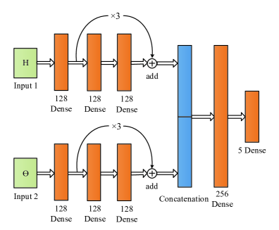
Different from the naive DQN method, where the DQN (with the weights ) is used to generate the target value, we use a separate target network (with the weights ) to generate the target value, and the weights of the target network are updated by in every time intervals. The structure of the network is shown in Figure 4. Specifically, we apply the deep residual network (ResNet) [40] to process two sub-states (i.e., and ), and then we fuse the processed information of the two sub-states using a two-layer dense network. The activation function that we use is the Swish function [41].
III-C2 -Greedy Policy
Given the perfect , the optimal policy is to select the action that yields the largest state-action value. However, the perfect demands for a infinite size of experiences, which is impractical and infeasible in the dynamic wireless environment. Therefore, it is necessary for the agent to keep exploring to avoid get stuck with a sub-optimal policy. To this end, we apply an -greedy policy. In -greedy policy, refers to the probability of choosing to explore, i.e., randomly select from all the possible actions, and is the probability of choosing to exploit the obtained DQN in decision making. In this regard, the -greedy policy is represented as
| (31) |
where as the policy based on the Q-network, which is introduced in (20). In our design, is initially set to and decreases exponentially at a rate of every time interval until its reaches the lower bound .
III-C3 Experience Replay
Instead of training the DQN with the latest experience tuple, we store recent experience tuples in the memory in “first in, first out” (FIFO) manner, i.e., queue data structure, and then randomly fetch a mini-batch of experience samples from to train the DQN.
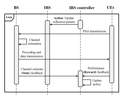
III-D Summarizing The Work Flow of Model-Free IRS Configuration
In this subsection, we summarize the work flow of the proposed model-free IRS configuration. To this end, we plot the sequence diagram in Figure 5.
According to Figure 5, in a specific loop, the IRS is configured with a reflection pattern () according to the -greedy policy, and then UEs and BS perform uplink pilot transmission and downlink data transmission sequentially as if there exists no IRS. After that, BS sends the estimated channel matrix () to IRS controller, which can be fulfilled through wired communications, and UEs send back their performance metrics to the IRS controller. Finally, according to the received channel estimate () and performance feedback (), IRS controller derives the tuple and stores it in the FIFO queue as the training data for the DQN .
Compared with the traditional TDD multi-user MIMO, the extra efforts of incorporating IRS are merely the feedback of and . The former can be easily achieved via wired communications between BS and IRS, and the latter costs negligible wireless communication resources of the mobile UEs. It is also noteworthy that IRS controller is unaware of the working mechanism of BS and UEs and does not require the CSI of the sub-channels.
IV Enhancing IRS Control Using Extremum Seeking Control
In DRL, action space is restrained for a fast convergence rate, which limits the phase freedom of IRS. To enhance the control of IRS, another model-free real-time optimization method, namely, extremum seeking control (ESC), is used to design the fine phase control of IRS.
IV-A Model-Free Control of IRS Using ESC
ESC is model-free method to realize a learning-based adaptive controller for maximizing/minimizing certain system performance metrics [42, 43]. The first application of ESC can be traced back to the work of the French engineer Leblanc in 1922 to maintain an efficient power transfer for a tram car [44]. The basic idea of ESC is to add a dither signal (e.g., sinusoidal signal [45, 46], and random noise [47]) to the system input and observing its effect on the output to obtain an approximate implicit gradient of a nonlinear static map of the unknown system [48, 42].
According to the design philosophy of ESC, we propose a dither-based model-free control of IRS as in Figure 6. Our design consists of three parts, i.e., dither signal generation module, ascent direction estimation module, and parameter update module. Dither signal generation module generates random dither/pertubation signal to probe the response of the system; gradient estimation module determines the update direction of the system input according to the system performance to guarantee the monotonic increase of the performance, and it also guides on-off switch of the random dither signal generation; parameter update module updates the system input according to the estimated direction.
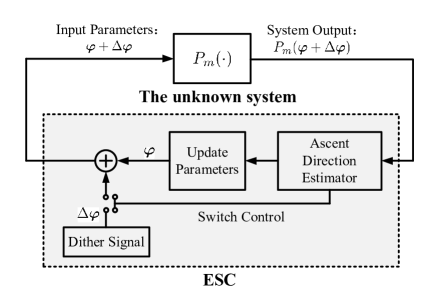
Specifically, the iterative process in Figure 6 runs as follows.
Step 1. Dither Signal Generation
Generate a small random dither signal through uniform random distribution222The parameter selection will be explained in the following context., i.e.,
| (32) |
Then, add the dither signal to the parameter , use as the input of the system, and receive the feedback of the performance metric .
Step 2. Direction Estimation and Parameter Update
Condition 1. If , adopt as the direction. Update the parameter as
| (33) |
and update the performance metric as
| (34) |
Then, jump to Step 1 for the next iteration;
Condition 2. Else if , adopt as the direction. Update the parameter as set
| (35) | ||||
Turn off the dither signal, use only as the system input, and measure the system performance . Then, jump to Step 1 for the next iteration.
It is noteworthy that each iteration uses one or two time intervals, and each iteration can guarantee the monotonic increase of the performance metric , which is validated in the following proposition.
Proposition 1.
Each iteration in ESC based iterative process can guarantee the monotonic increase of the performance metric given that the norm of the random dither signal, i.e., , is small enough.
Proof.
To prove Proposition 1, it is essential to validate that the operation (35) in Condition 2 of Step 2 guarantees the increase of , i.e., when , the following inequality
holds.
To this end, we expand using Taylor series of with respect to , i.e.,
| (36) |
Since is small, namely, , we adopt the first-order approximation, i.e.,
| (37) |
As it is reported by the system that in Condition 2, we have
| (38) |
Then, it is easy to verify that
| (39) |
∎
IV-B Comparison with Gradient Ascent Search
To obtain further insights into the proposed dither-based method, we make a comparison with the well-known iterative algorithm – gradient ascent (descent in minimization problems) search.
For gradient ascent search algorithm, in each iteration is updated as follows.
| (41) |
When the step size is small, the iteration will almost surely guarantee the increase of , because
| (42) |
Remark 3.
As gradient ascent search take steps in the direction of the gradient, it is also called steepest descent. Thus, the convergence rate of gradient ascent search is faster than dither-based extremum search when the step size is properly selected. On the other hand, it is also noteworthy that gradient ascent search requires the exact expression of the gradient , whilst dither-based method is implemented through trial and error, which does not rely on any explicit knowledge of the wireless system’s internal working mechanism.
IV-C Integrating ESC Into DRL
Recall that the action space for DRL is intentionally restrained for a fast convergence rate, whilst dither-based iterative method relies on the small-scale phase shift. Therefore, dither-based iterative method is complementary to the action in DRL and can be applied to enhance the action of DRL.
The enhanced action of DRL is defined as follows.
Step 1. Coarse phase shift (CPS) When , set
| (43) |
where is the reflection pattern at the -th channel block, is the coarse incremental phase shift at the -th channel block, and is the intermediate reflection pattern at the -th channel block. Following the example in Section III. C, the action set of the incremental phase shift is .
Step 2. Fine phase shift (FPS)
For from to , do
| (44) |
where is the ascent direction, and is the random dither signal.
Remark 4.
For example, when the quantization level , and , the step of coarse phase shift is , and the step of fine phase shift is with the range .
To be compatible with the enhanced action, the frame structure needs to be updated as in Figure 7. In the first time slots, UEs transmit pilots and BS performs channel estimation with the reflection pattern in (43), and in the subsequent time slots, UEs repeatedly transmit pilots and BS performs channel estimation, while the reflection pattern updates as in (44). It is noteworthy that, as the performance feedback is done once per channel block, the performance metric used for the dither-based method is an approximation derived by replacing the authentic channel response in (10) with the channel estimate .
Remark 5.
The parameter can be set adaptively according to the channel dynamics. For a practical wireless communication system, different values of correspond to different modes.
V Numerical Results
In this section, we present some numerical results to verify the effectiveness of our proposed model-free control of IRS 333The simulation code is available at https://github.com/WeiWang-WYS/IRSconfigurationDRL.
V-A Simulation Parameters
The BS is equipped with a ULA that is placed along the direction (i.e., x-axis), and IRS is a ULA, which is placed along the direction (i.e., y-axis), UEs are equipped with a single antenna, the user number is , BS antenna number is , and IRS reflector number if . The element antennas/reflectors of BS and IRS are both with half wavelength spacing. The position of BS is , the position of IRS is , and the UEs are uniformly distributed in the area with the height being . The noise variance at BS side is , the noise variance at UE side is . Each channel episode consists of channel blocks. In each channel episode, the LoS component is generated by randomly selecting the user locations within the area , and the LoS component is time-invariant within the channel blocks of that channel episode.
The LoS channel between BS and IRS is
| (45) |
where the steering vectors are represented as
and, according to [49], the directional cosines are given by
| (47a) | ||||
| (47b) | ||||
where the direction vector is determined by the relative position of BS and UE, i.e.,
| (48) |
The NLoS components are Gaussian distributed, i.e., . The channel matrix and are generated in the same way.
V-B Performance Study of DRL
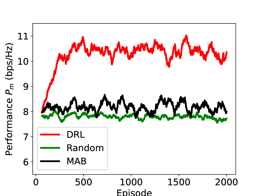
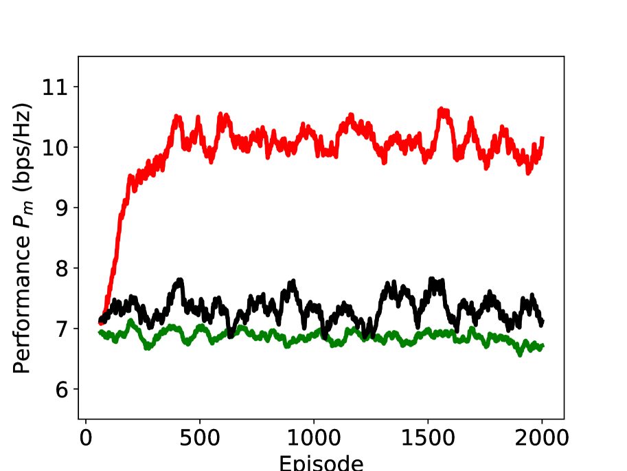
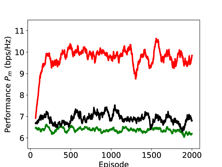
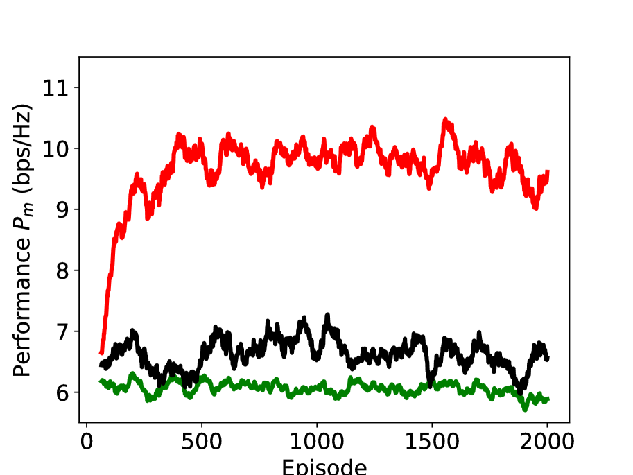
In Figure 8, we study the performance of the proposed DRL scheme (with the action set ) under different values of Rician factor. The x-axis represents the episode, and the y-axis represents the moving average of (window length is ). As can be seen, the proposed DRL significant outperforms the benchmark schemes, i.e., random reflection and multi-armed bandit (MAB). Different from DRL, the actions of random reflection and MAB that we used are absolute phase shift, and the action set is the DFT vectors. Although all the three schemes are independent of the sub-channel CSI, their utilizations of the other information are different. Random reflection is independent of any information and undoubtedly achieves the worst performance; MAB assumes a fixed distribution of rewards and explores the reward distributions of all arms. However, MAB fails to describe the state of the environment and to build the connection between the action and the environment; DRL defines an appropriate state to represent the agent’s “position” within the environment and learns the quality of a state-action combination using the DQN from the information of rewards and states, which enables the agent to choose the best action to maximize the returns. We can also find that the performance gap of DRL and the benchmarks schemes becomes larger with the increase of Rician factor , which indicates that the effectiveness of DRL is also dependent on the radio environment.
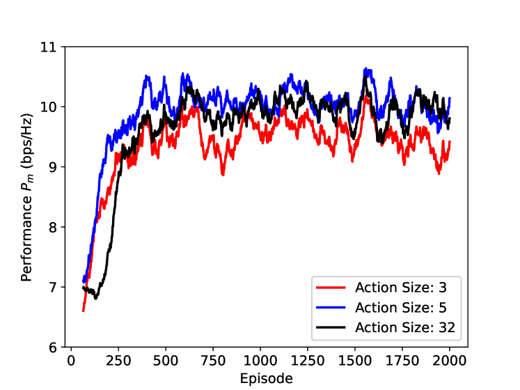
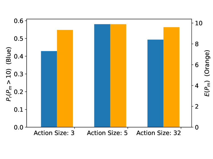
In Figure 9, we study the impacts of action size to the performance of the proposed DRL scheme when the Rician factor is . In addition to the action set defined in Section III, we adopt the action set and action set (namely, DFT matrix) as the benchmarks. From Figure 9, we can see that is the fastest to converge, while is the slowest. Although a large action size will speed up the response rate of the agent, it will, on the other hand, demand more time for the DQN to converge. In the convergence region, we find that and achieve the similar performance, while ’s performance is inferior. It indicates that a well-design action set with a moderate size might be better than the small action size and the over-large action size. In Figure 9, the average sum rate , and the probability are presented in the bar chart. For , bps/Hz and ; for , bps/Hz and ; for , bps/Hz and . It further verifies the importance of action set design.
V-C Performance Study of ESC
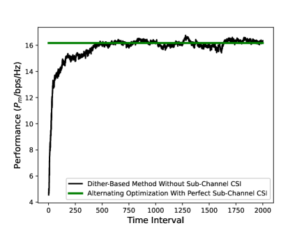
In Figure 10, we study the performance of the ESC-inspired dither-based iterative method in a specific channel block. Each time interval of -axis consists of time slots, which is the pilot length required by the BS to estimate the multi-user channel . As can be seen that the performance metric for dither-based method is almost monotonically increasing over time. Note that the performance metric used to guide the dither-based iterative method is an approximation, rather than the authentic feedback. Thus, the slight fluctuation of the performance curve is reasonable. For the purpose of comparison, we adopt the model-based method as the benchmark, in which the perfect sub-channel CSI, namely, , , and , is available. The optimal reflection coefficient vector is derived through solving the optimization problem (3). Recall that the difference from model-free control is that the exact relationship between the objective function and the variable is known in model-based methods. Due to the discrete nature of the feasible region , the optimization problem is intractable. Hence, we manage to solve it using the alternating optimization technique, which alternatively freezes reflection coefficients and optimize only reflection coefficient. According to Figure 10, the model-free dither-based method achieves almost the same performance as the model-based alternating optimization when the time index is greater than . However, in practice, we have to weigh the cost of time resources against the benefits. As the dither-based method needs to sample , one iteration means the cost of a unit of time resource in wireless communications. Thus, in order to balance the time allocation between pilot transmission and data transmission, the time resources dedicated to dither-based method (i.e., the time for pilot transmission) should be deliberately selected according to channel dynamics (i.e., the length of a channel block).
V-D Performance Study of the Integrated DRL and ESC
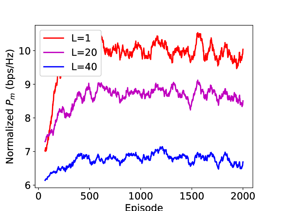
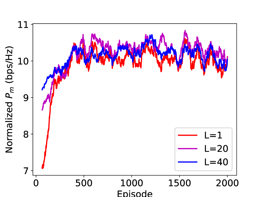
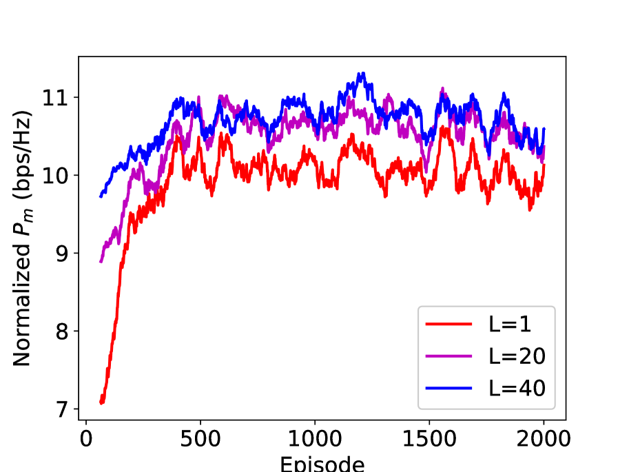
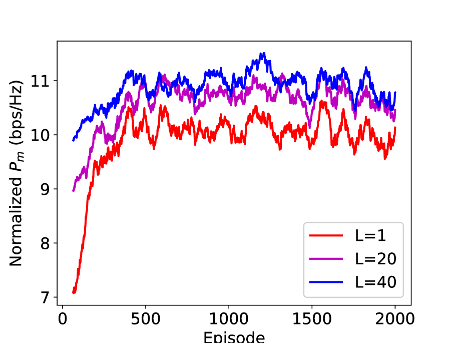
In Figure 11, we study the performance of the integrated DRL and ESC method (with the action set ) in different channel dynamics. The normalized is the obtained by multiplying by the coefficient , where is the channel block length and is the training length. Take and as an example, the first time interval is used for pilot transmission and the rest time intervals are used for data transmission. It is also noteworthy that when the scheme is DRL only, and when the scheme is the integrated DRL and ESC. In addition, we adopt the action set . From the figure, we can see that when the channel block length , DRL outperforms the integrated DRL and ESC with . However, when the channel block length increases, the integrated DRL and ESC gradually becomes superior, which verifies its effectiveness in the slow fading channel. Therefore, the parameter of the integrated DRL and ESC can be set adaptively to accommodate different channel dynamics.
VI Conclusion
In this paper, we have proposed a model-free control of IRS that is independent of sub-channel CSI. We firstly model the control of IRS as an MDP and apply DRL to perform real-time coarse phase control of IRS. Then, we apply ESC as the fine phase control of IRS. Finally, by updating the frame structure, we integrate DRL and ESC in the model-free control of IRS to improve its adaptivity to different channel dynamics. Numerical results show the superiority of our proposed scheme in model-free IRS control without sub-channel CSI.
References
- [1] N. Engheta and R. W. Ziolkowski, Metamaterials: Physics and Engineering Explorations. John Wiley & Sons, 2006.
- [2] T. J. Cui, M. Q. Qi, X. Wan, J. Zhao, and Q. Cheng, “Coding metamaterials, digital metamaterials and programmable metamaterials,” Light Sci. Appl., vol. 3, no. 10, pp. e218–e218, Oct. 2014.
- [3] D. Schurig, J. J. Mock, B. Justice, S. A. Cummer, J. B. Pendry, A. F. Starr, and D. R. Smith, “Metamaterial electromagnetic cloak at microwave frequencies,” Science, vol. 314, no. 5801, pp. 977–980, Nov. 2006.
- [4] L. Liang, M. Qi, J. Yang, X. Shen, J. Zhai, W. Xu, B. Jin, W. Liu, Y. Feng, C. Zhang et al., “Anomalous terahertz reflection and scattering by flexible and conformal coding metamaterials,” Adv. Opt. Mater., vol. 3, no. 10, pp. 1374–1380, Oct. 2015.
- [5] N. Yu, P. Genevet, M. A. Kats, F. Aieta, J.-P. Tetienne, F. Capasso, and Z. Gaburro, “Light propagation with phase discontinuities: generalized laws of reflection and refraction,” Science, vol. 334, no. 6054, pp. 333–337, Oct. 2011.
- [6] C. Zhang, W. Chen, Q. Chen, and C. He, “Distributed intelligent reflecting surfaces-aided device-to-device communications system,” J. Comm. Inform. Networks, vol. 6, no. 3, pp. 197–207, 2021.
- [7] M. Di Renzo et al., “Smart radio environments empowered by reconfigurable AI meta-surfaces: An idea whose time has come,” EURASIP J. Wireless Commun. Netw., vol. 2019, no. 1, pp. 1–20, 2019.
- [8] Q. Wu, S. Zhang, B. Zheng, C. You, and R. Zhang, “Intelligent reflecting surface aided wireless communications: A tutorial,” IEEE Trans. Commun., vol. 69, no. 5, pp. 3313–3351, May 2021.
- [9] Z. Wang, L. Liu, and S. Cui, “Channel estimation for intelligent reflecting surface assisted multiuser communications,” in 2020 IEEE Wireless Communications and Networking Conference (WCNC), 2020, pp. 1–6.
- [10] P. Wang, J. Fang, W. Zhang, and H. Li, “Joint active and passive beam training for IRS-assisted millimeter wave systems,” arXiv preprint arXiv:2103.05812, 2021.
- [11] P. Wang, J. Fang, H. Duan, and H. Li, “Compressed channel estimation for intelligent reflecting surface-assisted millimeter wave systems,” IEEE Signal Process. Lett., vol. 27, pp. 905–909, May 2020.
- [12] Q. Wu and R. Zhang, “Intelligent reflecting surface enhanced wireless network via joint active and passive beamforming,” IEEE Trans. Wireless Commun., vol. 18, no. 11, pp. 5394–5409, Nov. 2019.
- [13] D. Tse and P. Viswanath, Fundamentals of Wireless Communication. Cambridge University Press, 2005.
- [14] C. Qi, P. Dong, W. Ma, H. Zhang, Z. Zhang, and G. Y. Li, “Acquisition of channel state information for mmWave massive MIMO: Traditional and machine learning-based approaches,” Sci. China Inf. Sci, vol. 64, no. 8, pp. 1–16, 2021.
- [15] F. Liu, J. Pan, X. Zhou, and G. Y. Li, “Atmospheric ducting effect in wireless communications: Challenges and opportunities,” J. Comm. Inform. Networks, vol. 6, no. 2, pp. 101–109, 2021.
- [16] W. Wang and W. Zhang, “Joint beam training and positioning for intelligent reflecting surfaces assisted millimeter wave communications,” IEEE Trans. Wireless Commun., vol. 20, no. 10, pp. 6282–6297, Oct. 2021.
- [17] H. Yang et al., “A programmable metasurface with dynamic polarization, scattering and focusing control,” Sci. Rep., vol. 6, no. 1, pp. 1–11, Oct. 2016.
- [18] W. Tang et al., “Wireless communications with programmable metasurface: Transceiver design and experimental results,” China Commun., vol. 16, no. 5, pp. 46–61, May 2019.
- [19] Q. Wu and R. Zhang, “Joint active and passive beamforming optimization for intelligent reflecting surface assisted SWIPT under QoS constraints,” IEEE J. Sel. Areas in Commun., vol. 38, no. 8, pp. 1735–1748, Aug. 2020.
- [20] Y. Yang, S. Zhang, and R. Zhang, “IRS-enhanced OFDM: Power allocation and passive array optimization,” in 2019 IEEE Global Communications Conference (GLOBECOM). IEEE, 2019, pp. 1–6.
- [21] X. Yu, D. Xu, D. W. K. Ng, and R. Schober, “IRS-assisted green communication systems: Provable convergence and robust optimization,” IEEE Trans. Commun., vol. 69, no. 9, pp. 6313–6329, Sept. 2021.
- [22] K. Zhi, C. Pan, H. Ren, and K. Wang, “Ergodic rate analysis of reconfigurable intelligent surface-aided massive MIMO systems with ZF detectors,” IEEE Commun. Lett., vol. 26, no. 2, pp. 264–268, Feb. 2022.
- [23] Y. Han, W. Tang, S. Jin, C.-K. Wen, and X. Ma, “Large intelligent surface-assisted wireless communication exploiting statistical CSI,” IEEE Trans. Veh. Technol., vol. 68, no. 8, pp. 8238–8242, Aug. 2019.
- [24] K. Zhi, C. Pan, G. Zhou, H. Ren, M. Elkashlan, and R. Schober, “Is RIS-aided massive MIMO promising with ZF detectors and imperfect CSI?” arXiv preprint arXiv:2111.01585, 2021.
- [25] K. Zhi, C. Pan, H. Ren, K. Wang, M. Elkashlan, M. Di Renzo, R. Schober, H. V. Poor, J. Wang, and L. Hanzo, “Two-timescale design for reconfigurable intelligent surface-aided massive MIMO systems with imperfect CSI,” arXiv preprint arXiv:2108.07622, 2021.
- [26] M.-M. Zhao, Q. Wu, M.-J. Zhao, and R. Zhang, “Intelligent reflecting surface enhanced wireless networks: Two-timescale beamforming optimization,” IEEE Trans. Wireless Commun., vol. 20, no. 1, pp. 2–17, Jan. 2021.
- [27] A. Taha, Y. Zhang, F. B. Mismar, and A. Alkhateeb, “Deep reinforcement learning for intelligent reflecting surfaces: Towards standalone operation,” in 2020 IEEE 21st International Workshop on Signal Processing Advances in Wireless Communications (SPAWC). IEEE, 2020, pp. 1–5.
- [28] A. Taha, M. Alrabeiah, and A. Alkhateeb, “Enabling large intelligent surfaces with compressive sensing and deep learning,” IEEE Access, vol. 9, pp. 44 304–44 321, 2021.
- [29] B. Sheen, J. Yang, X. Feng, and M. M. U. Chowdhury, “A deep learning based modeling of reconfigurable intelligent surface assisted wireless communications for phase shift configuration,” IEEE Open J. Commun. Soc., vol. 2, pp. 262–272, 2021.
- [30] Y. Kim, G. Miao, and T. Hwang, “Energy efficient pilot and link adaptation for mobile users in TDD multi-user MIMO systems,” IEEE Trans. Wireless Commun., vol. 13, no. 1, pp. 382–393, Jan. 2013.
- [31] W. Zhang, H. Ren, C. Pan, M. Chen, R. C. de Lamare, B. Du, and J. Dai, “Large-scale antenna systems with UL/DL hardware mismatch: Achievable rates analysis and calibration,” IEEE Trans. Commun., vol. 63, no. 4, pp. 1216–1229, Apr. 2015.
- [32] A. Goldsmith, Wireless Communications. Cambridge University Press, 2005.
- [33] A. K. Samingan, I. Suleiman, A. A. A. Rahman, and Z. M. Yusof, “LTF-based vs. pilot-based MIMO-OFDM channel estimation algorithms: An experimental study in 5.2 GHz wireless channel,” in 2009 IEEE 9th Malaysia International Conference on Communications (MICC), 2009, pp. 794–800.
- [34] R. S. Sutton and A. G. Barto, Reinforcement Learning: An Introduction. MIT press, 2018.
- [35] L. P. Kaelbling, M. L. Littman, and A. W. Moore, “Reinforcement learning: A survey,” J. Mach. Learn. Res., vol. 4, pp. 237–285, May 1996.
- [36] K. Arulkumaran, M. P. Deisenroth, M. Brundage, and A. A. Bharath, “Deep reinforcement learning: A brief survey,” IEEE Signal Process. Mag., vol. 34, no. 6, pp. 26–38, Nov. 2017.
- [37] V. Mnih, K. Kavukcuoglu, D. Silver, A. A. Rusu, J. Veness, M. G. Bellemare, A. Graves, M. Riedmiller, A. K. Fidjeland, G. Ostrovski et al., “Human-level control through deep reinforcement learning,” Nature, vol. 518, no. 7540, pp. 529–533, Feb. 2015.
- [38] V. Mnih, K. Kavukcuoglu, D. Silver, A. Graves, I. Antonoglou, D. Wierstra, and M. Riedmiller, “Playing atari with deep reinforcement learning,” arXiv preprint arXiv:1312.5602, 2013.
- [39] H. Van Hasselt, A. Guez, and D. Silver, “Deep reinforcement learning with double Q-learning,” in Proceedings of the AAAI Conference on Artificial Intelligence (AAAI), vol. 30, no. 1, 2016.
- [40] K. He, X. Zhang, S. Ren, and J. Sun, “Deep residual learning for image recognition,” in Proceedings of the IEEE conference on Computer Vision and Pattern Recognition, 2016, pp. 770–778.
- [41] P. Ramachandran, B. Zoph, and Q. V. Le, “Searching for activation functions,” arXiv preprint arXiv:1710.05941, 2017.
- [42] K. B. Ariyur and M. Krstić, Real-Time Optimization by Extremum-Seeking Control. John Wiley & Sons, 2003.
- [43] Nešić et al., “A framework for extremum seeking control of systems with parameter uncertainties,” IEEE Trans. Autom. Control, vol. 58, no. 2, pp. 435–448, Feb. 2013.
- [44] Y. Tan, W. Moase, C. Manzie, D. Nešić, and I. Mareels, “Extremum seeking from 1922 to 2010,” in Proceedings of the 29th Chinese Control Conference, 2010, pp. 14–26.
- [45] H.-H. Wang, M. Krstić, and G. Bastin, “Optimizing bioreactors by extremum seeking,” Int. J. Adapt. Control Signal Process., vol. 13, no. 8, pp. 651–669, 1999.
- [46] D. Nešić, “Extremum seeking control: Convergence analysis,” Eur. J. Control, vol. 15, no. 3-4, pp. 331–347, 2009.
- [47] D. Carnevale et al., “Maximizing radiofrequency heating on FTU via extremum seeking: parameter selection and tuning,” in From Physics to Control Through an Emergent View. World Scientific, 2010, pp. 321–326.
- [48] K. T. Atta, A. Johansson, and T. Gustafsson, “Extremum seeking control based on phasor estimation,” Syst. Control Lett., vol. 85, pp. 37–45, Nov. 2015.
- [49] W. Wang and W. Zhang, “Jittering effects analysis and beam training design for UAV millimeter wave communications,” IEEE Trans. Wireless Commun., pp. 1–1, 2021.