Intelligent Reflecting Surface-Aided Maneuvering Target Sensing: True Velocity Estimation
Abstract
Maneuvering target sensing will be an important service of future vehicular networks, where precise velocity estimation is one of the core tasks. To this end, the recently proposed integrated sensing and communications (ISAC) provides a promising platform for achieving accurate velocity estimation. However, with one mono-static ISAC base station (BS), only the radial projection of the true velocity can be estimated, which causes serious estimation error. In this paper, we investigate the estimation of the true velocity of a maneuvering target with the assistance of an intelligent reflecting surface (IRS). We propose an efficient velocity estimation algorithm by exploiting the two perspectives from the BS and IRS to the target. We propose a two-stage scheme where the true velocity can be recovered based on the Doppler frequency of the BS-target link and BS-IRS-target link. Experimental results validate that the true velocity can be precisely recovered and demonstrate the advantage of adding the IRS.
Index Terms:
Intelligent reflecting surface, integrated sensing and communications, Doppler effect, true velocity estimation.I Introduction
Vehicular to everything (V2X) communications is becoming a key enabling technology for many thrilling applications, e.g., smart city and intelligent transportation systems. However, V2X poses stringent requirements on both sensing accuracy and communication quality. To this end, the recently proposed integrated sensing and communication (ISAC) provides a promising platform that amalgamates the abilities of sensing and communication, especially for 5G and beyond systems [1, 2, 3]. However, high-accuracy beam tracking is necessary to compensate for the path loss imposed by the high-frequency signals and guarantee the quality-of-service (QoS) for V2X, particularly in high-mobility vehicular scenarios [4].
To achieve accurate beam-tracking, precise velocity estimation is required. Doppler effect, which refers to the change in frequency of an electromagnetic wave caused by the relative motion between the observer and the wave source, is typically utilized for velocity estimation. Existing works on velocity estimation mainly adopted matched filters (MFs) to estimate the motion parameters [5, 6, 4]. Micro-Doppler frequency estimation was considered in [5] for orthogonal frequency division multiplexing (OFDM) radar systems. In [6], the authors proposed to mitigate the inter-carrier interference caused by the Doppler effect to improve the performance of Doppler estimation by oversampling. A predictive beamforming design was investigated for an ISAC system in [4]. In general, the performance of the MF-based method is limited by the inherent grid issue. To address this problem, a joint range-velocity estimation was proposed in [7] based on the multiple signal classification (MUSIC) algorithm in OFDM radar systems, which achieves a higher resolution than the MF-based methods. However, due to the nature of the Doppler effect, the conventional mono-static ISAC BS can only measure the radial projection of the true velocity, and thus the true velocity cannot be uniquely recovered. One solution is to obtain another perspective toward the maneuvering target so that the true velocity can be uniquely determined.
In recent years, intelligent reflecting surfaces (IRSs) have been introduced to enhance the performance of both communication and sensing [8, 9, 10]. Some research efforts have been made to IRS-aided systems to tackle user equipment (UE) mobility [11, 12, 13]. The authors in [11] considered a continuous model for IRS-aided satellite communication, based on which the IRS phase shifters are optimized to simultaneously maximize the received power and minimize the delay and Doppler spread. In [12], a two-stage protocol for channel estimation was proposed for an IRS-aided high-mobility communication system, which deploys an IRS at a high-speed vehicle to enhance the QoS for passengers by mitigating the Doppler effect. In [13], the authors considered the localization problem in an IRS-aided single-input single-output (SISO) system by taking into account the UE mobility and spatial wideband effects. However, the potential of IRSs for true velocity estimation has not been fully understood.
In this paper, by leveraging the additional perspective provided by the IRS, we study the true velocity estimation in an IRS-aided ISAC system. By exploiting the geometric information, the true velocity can be recovered based on the Doppler frequency of the BS-target link and BS-IRS-target link111For simplicity, we will refer to the BS-target link and BS-IRS-target link as the direct link and IRS link, respectively.. To estimate the Doppler frequency of both links, we propose a two-stage scheme. In the first stage, a coarse estimation of radial projection of the true velocity is obtained by turning off the IRS. In the second stage, a gridless estimation for the Doppler frequency of the direct link and IRS link is performed by exploiting the method of direction estimation (MODE) [14]. Compared with existing gridless estimation methods such as root-multiple signal classification (root-MUSIC) [15] and estimation of signal parameters via rotation invariance techniques (ESPRIT) [16], the MODE approach is shown to provide more accurate parameter estimation [14].
II Preliminary
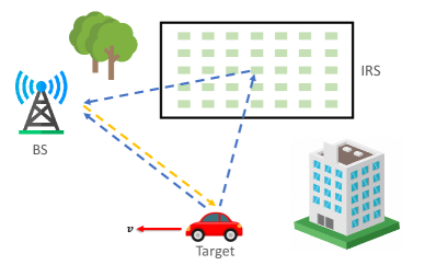
Consider an ISAC system, as illustrated in Fig. 1, where the velocity vector of the point-like maneuvering target, denoted by 222The velocity vector is defined by , where represents the direction of velocity as illustrated in Fig. 2., is estimated by one BS with the help of an IRS. The BS and IRS are equipped with a uniform linear array (ULA) with and antennas, respectively.
II-A Signal Model
Assume that the directions of the target with respect to the BS and IRS, denoted by and in Fig. 2(b), are well estimated in advance. To estimate the true velocity, the BS transmits a probing beam
| (1) |
where and represent the inner spacing of the ULA and the wavelength, respectively. Here, represents the steering vector of the antenna array of the BS towards the target. Note that due to the use of the narrow beam, the effect of the non-light-of-sight (NLoS) path is considered negligible.
The echo of the -th pilot symbol received by the BS is given by
| (2) |
where
| (3) |
represents the response vector of the IRS, denotes the channel between BS and IRS, which is modeled as a Rician channel comprising a light-of-sight (LoS) path and a number of NLoS paths, denotes the phase shifter which is designed to align toward the target333The optimized design of phase shifter will be left as future work., and denote the complex channel gain, accounting for the path loss and target reflectivity444The fluctuations of target reflectivity are typically modeled using the standard Swerling classes. In this paper, we adopt the Swerling I model where the reflectivity is assumed to be constant within a symbol [17].. and represent the Doppler frequencies corresponding to the direct link and IRS link, respectively, denotes the symbol period, and denote the noise vectors whose elements are drawn independently from a complex Gaussian distribution with zero mean and covariance matrix [13].
II-B Geometrical Insights of Doppler Effect
Since the Doppler effect depends on the mobility of the target, we propose to estimate the true velocity by exploiting the Doppler frequencies .In the following, we first discuss the geometrical insights of the Doppler effect to reveal the relation between true velocity and the Doppler frequencies .
The Doppler frequency of the relative motion between the BS and the maneuvering target is given by
| (4) |
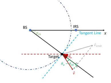
where denotes the amplitude of the true velocity, and represents the angle between the velocity direction and the -axis, which is marked in red in Fig. 2. Note that is the projection of velocity on the line across the BS and target, which is marked in dark green in Fig. 2(a). Then, the Doppler frequency corresponding to the direct link is given by
| (5) |
The deployment of the IRS creates another path, which allows the BS to observe the velocity from an additional perspective. The Doppler frequency of the relative motion between the IRS and the maneuvering target is given by
| (6) |
Then, the Doppler frequency corresponding to the IRS link is given by
| (7) |
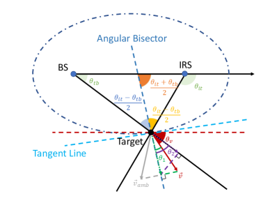
where and which are marked in dark green and purple in Fig. 2(b), respectively.
From (7), comes from two projections:
-
1.
: This term projects the velocity to the angular bisector of the angle . Note that the angular bisector is perpendicular to the tangent line of the ellipse with foci at the BS and IRS.
-
2.
: This term projects the projected speed to the line connecting the BS and the target (or the line connecting the IRS and the target). Since the direction of the projected speed is fixed, there will be no ambiguity on the velocity at the projection corresponding to .
Remark: The conventional mono-static radar can only access , which corresponds to the radial component of the velocity. As a result, the tangent projection will cause ambiguity, e.g., different velocities may yield the same observation at the BS. One example is illustrated in Fig. 2(a) where two velocity vectors, i.e., (marked in gray) and (marked in red), give the same projection. Similarly, for the IRS link, the velocity ambiguity occurs at the tangent line of the ellipse, as illustrated in Fig. 2(b). Thus, either of the two links, by itself, will cause velocity ambiguity. Nevertheless, by jointly considering the two links, the true velocity vector can be uniquely determined. Note that we assume that the distance between the BS and the IRS should be comparable to the distance between the target and the BS/IRS.
The following proposition provides the true velocity estimation in the IRS-aided system by jointly leveraging and .
Proposition 1
The direction and absolute value of the true velocity can be determined uniquely as
| (8) |
| (9) |
Proof: See Appendix.
III True Velocity Estimation
According to Proposition 1, to estimate the true velocity, we need to estimate and . In this section, we propose a two-stage scheme to estimate the true velocity of the maneuvering target. Specifically, in the first stage, we obtain a coarse estimation of . In the second stage, and are estimated accurately by utilizing the MODE. The coarse estimation serves two purposes. First, it can be utilized to initialize the iterative algorithm to speed up the iteration in the second stage. Second, the coarse estimation can help match the estimated Doppler frequencies to different links.
III-A Stage I: Coarse Estimation of
We first turn off the IRS to obtain a coarse estimation of only based on the direct link. This can be implemented through a receiving beam with zero gain on the direction of IRS. In this case, the system degenerates to a conventional mono-static one. Assume the BS transmits pilot symbols in Stage I. Given the pilot symbol , the received echo of the -th symbol at the BS is given by
| (10) |
where denotes the noise vector whose elements are drawn independently from a complex Gaussian distribution with zero mean and covariance matrix
Define as the combiner corresponding to the received beam which points to the estimated target position. Then the output for the -th symbol is given by
| (11) |
where and denotes the combined noise following the Gaussian distribution, i.e., . Stacking into a vector yields
| (12) |
Define the steering vector in the Doppler domain as
| (13) |
The coarse estimation of is obtained as
| (14) |
III-B Stage II: Refined Gridless Estimation of and
At this stage, we turn on the IRS to obtain a refined estimation of and . The BS transmits pilot symbols at this stage. Define as the combiner illuminated at the estimated target position and IRS, simultaneously, where denotes the direction of the IRS with respect to the BS. Then, the output for the -th symbol is given by
| (15) |
where and denotes the combined noise, which follows the Gaussian distributions, i.e., .
Before proceeding, we first construct a set of signal vectors by rearranging . By doing that, the Doppler frequency estimation problem can be solved by the MODE. Given a positive integer , the signal vector is defined as
| (16) |
From (15), (16) can be rewritten as
| (17) |
where
| (18) |
| (19) |
| (20) |
The covariance matrix of is
| (21) |
where denotes the expectation over and . The eigenvalue decomposition of gives
| (22) |
where are the eigenvalues, and correspond to the signal and noise subspace, respectively. Note that the linear span of is the same as that of , i.e.,
| (23) |
Note that the maximum likelihood estimate (MLE) of depends on , which is unknown in practice. To address this, we first obtain the estimated eigenvectors and the estimated eigenvalues by performing the eigenvalue decomposition on the sample covariance matrix of , i.e.,
| (24) |
Then, an approximated maximum likelihood estimate (MLE) of is given by [14]
| (25) |
where denotes the trace, represents the orthogonal projector onto the range space of , and , while
| (26) |
and .
However, the problem in (25) does not have an analytical solution and is thus hard to solve directly. To solve (25), we then consider introducing some tractable intermediate variables, based on which and can be estimated. Construct a polynomial
| (27) |
which has roots in the complex plane. It can be validated that and . Clearly, and are the roots of this polynomial. Then, the strategy of solving (25) is to obtain the intermediate variables and , based on which and can be estimated, instead of estimating and directly.
Recall from (27) that is related to . Then, the MLE of is given by
| (32) |
Define matrix
| (33) |
and vector
| (34) |
where denotes the -th entry of . We have
| (35) |
where
| (36) |
| (37) |
Substituting (35) into (32) leads to
| (38) |
Note that (38) is a weighted least squares problem whose solution is given by
| (39) |
However, also depends on through (31) and (28). In order to tackle this challenge, we propose an iterative algorithm to find the solution, which is summarized in Algorithm 1.
Once is obtained, we can solve the equation
| (40) |
to obtain two roots
| (41) |
The corresponding and are obtained as
| (42) |
where denotes the phase of a complex number.
We can obtain the refined estimates of and , i.e.,
| (43) |
By exploiting Proposition 1, the direction and absolute value of true velocity can be estimated.
IV Simulation Results
In this section, we show the performance of the proposed velocity estimator. The number of antennas at the BS is set as and the number of elements at the IRS is set as . The carrier frequency is GHz and the symbol period is ms. The number of symbols at stages I and II are and , respectively. Assume that the BS and IRS are located at and , respectively, where all coordinates are in meters. The direction of the target with respect to the BS and IRS are and , respectively. is modeled as a Rician channel comprising a LOS path and a number of NLOS paths. The number of paths for is set as , where the AoA and AoD parameters are uniformly generated from . The Rician factor is set as dB. The signal-to-noise ratio (SNR) of the direct link is defined as .
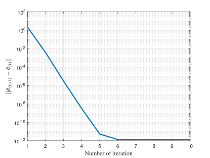
We first show the convergence performance of the proposed MODE-based method, which involves an iterative process. For that purpose, we choose the average discrepancy of between two adjacent iterations as the metric, i.e., For each abscissa, Monte-Carlo trials are carried out. From Fig. 3, we can see that the iteration converges in about ten rounds.
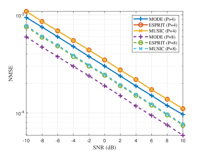
We compare the proposed MODE-based method with two gridless alternatives, i.e., root-MUSIC [15] and root-ESPRIT [16]. To quantify the estimation accuracy, we evaluate the normalized mean squared error (NMSE), i.e., where denotes the number of Monte-Carlo trials and denotes the estimation result in the -th Monte-Carlo trial.
The NMSEs of different methods under different SNRs are shown in Fig. 4. The velocity of target is m/s with and . From Fig. 4, we observe that the true velocity can be recovered with a considerable accuracy. As SNR increases, the NMSEs of all these methods decrease. Furthermore, the proposed MODE can achieve higher accuracy than MUSIC and ESPRIT. This is because the MODE can achieve the minimum estimation variance among the class of methods based on the eigenspace of the sample covariance matrix including MUSIC and ESPRIT [14].
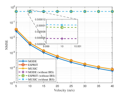
Next, we show the NMSE performance under different target velocities in Fig. 5. We set , , and dB. From Fig. 5, we can see that the NMSE performance is significantly improved with the deployment of the IRS. This is because only a radial projection of the true velocity can be estimated for a single BS without the IRS, such that the tangent projection of the true velocity dominates the estimation error. Meanwhile, with the IRS, the NMSE performance improves as the target velocity increases. The reason for this phenomenon requires a further theoretical study on the Cramér-Rao bound, which will be left to our future work. Moreover, the gap between the curves with and without the IRS becomes larger as increases, which indicates that the benefit of the deployment of IRSs will be more pronounced in the high-mobility case.
V Conclusion
This paper considered the true velocity estimation for a maneuvering target with the assistance of an IRS. Thanks to the extra link provided by the IRS, the BS can observe the true velocity from two different perspectives. In particular, we proposed a two-stage algorithm to estimate the Doppler frequency of the direct link and IRS link, based on which the true velocity recovered. Compared with existing approaches, the proposed approach achieved much better estimation performance. The work in this paper represents a small step to fully exploit the power of IRS in ISAC applications.
Proof of Proposition 1
(9) can be directly obtained from (5), thus we only prove (8) in the following. Recalling the definition of and , we have
| (44) |
Then, (5) can be reformulated as
| (45) |
According to (7), we have
| (46) |
References
- [1] F. Liu, C. Masouros, A. P. Petropulu, H. Griffiths, and L. Hanzo, “Joint radar and communication design: Applications, state-of-the-art, and the road ahead,” IEEE Trans. Commun., vol. 68, no. 6, pp. 3834–3862, Feb. 2020.
- [2] L. Xie, P. Wang, S. Song, and K. B. Letaief, “Perceptive mobile network with distributed target monitoring terminals: Leaking communication energy for sensing,” IEEE Trans. Wireless Commun., Jun. 2022.
- [3] L. Xie, S. Song, Y. C. Eldar, and K. B. Letaief, “Collaborative sensing in perceptive mobile networks: Opportunities and challenges,” arXiv preprint arXiv:2205.15805, 2022.
- [4] F. Liu, W. Yuan, C. Masouros, and J. Yuan, “Radar-assisted predictive beamforming for vehicular links: Communication served by sensing,” IEEE Trans. Wireless Commun., vol. 19, no. 11, pp. 7704–7719, Aug. 2020.
- [5] S. Sen, “Adaptive OFDM radar waveform design for improved micro-Doppler estimation,” IEEE Sens. J., vol. 14, no. 10, pp. 3548–3556, Jul. 2014.
- [6] J. Lim, S.-R. Kim, and D.-J. Shin, “Two-step Doppler estimation based on intercarrier interference mitigation for OFDM radar,” IEEE Antennas Wirel. Propag. Lett., vol. 14, pp. 1726–1729, Apr. 2015.
- [7] S. H. Dokhanchi, B. S. Mysore, K. V. Mishra, and B. Ottersten, “A mmwave automotive joint radar-communications system,” IEEE Trans. Aerosp. Electron. Syst., vol. 55, no. 3, pp. 1241–1260, Feb. 2019.
- [8] X. Yu, D. Xu, D. W. K. Ng, and R. Schober, “IRS-assisted green communication systems: Provable convergence and robust optimization,” IEEE Trans. Commun., vol. 69, no. 9, pp. 6313–6329, Jun. 2021.
- [9] X. Yu, V. Jamali, D. Xu, D. W. K. Ng, and R. Schober, “Smart and reconfigurable wireless communications: From IRS modeling to algorithm design,” IEEE Wireless Commun., vol. 28, no. 6, pp. 118–125, Dec. 2021.
- [10] J. He, H. Wymeersch, T. Sanguanpuak, O. Silvén, and M. Juntti, “Adaptive beamforming design for mmwave RIS-aided joint localization and communication,” in Proc. IEEE Wireless Commun. Netw. Conf. Workshops (WCNCW). IEEE, Jun. 2020, pp. 1–6.
- [11] B. Matthiesen, E. Björnson, E. De Carvalho, and P. Popovski, “Intelligent reflecting surface operation under predictable receiver mobility: A continuous time propagation model,” IEEE Wireless Commun. Lett., vol. 10, no. 2, pp. 216–220, Sep. 2020.
- [12] Z. Huang, B. Zheng, and R. Zhang, “Transforming fading channel from fast to slow: Intelligent refracting surface aided high-mobility communication,” IEEE Trans. Wireless Commun., Dec. 2021.
- [13] K. Keykhosravi, M. F. Keskin, G. Seco-Granados, P. Popovski, and H. Wymeersch, “RIS-enabled SISO localization under user mobility and spatial-wideband effects,” IEEE J. Sel. Topics Signal Process., May 2022.
- [14] P. Stoica and K. Sharman, “Maximum likelihood methods for direction-of-arrival estimation,” IEEE Trans. Acoustics, Speech, Signal Process., vol. 38, no. 7, pp. 1132–1143, Jul. 1990.
- [15] R. Schmidt, “Multiple emitter location and signal parameter estimation,” IEEE Trans. Antennas Propag., vol. 34, no. 3, pp. 276–280, Mar. 1986.
- [16] R. Roy and T. Kailath, “ESPRIT-estimation of signal parameters via rotational invariance techniques,” IEEE Trans. Acoustics, Speech, Signal Process., vol. 37, no. 7, pp. 984–995, Jul. 1989.
- [17] L. Xie, Z. He, J. Tong, and W. Zhang, “A recursive angle-Doppler channel selection method for reduced-dimension space-time adaptive processing,” IEEE Trans. Aerosp. Electron. Syst., vol. 56, no. 5, pp. 3985–4000, Apr. 2020.