Integrated Location Sensing and Communication for Ultra-Massive MIMO With Hybrid-Field Beam-Squint Effect
Abstract
The advent of ultra-massive multiple-input-multiple-output systems holds great promise for next-generation communications, yet their channels exhibit hybrid far- and near- field beam-squint (HFBS) effect. In this paper, we not only overcome but also harness the HFBS effect to propose an integrated location sensing and communication (ILSC) framework. During the uplink training stage, user terminals (UTs) transmit reference signals for simultaneous channel estimation and location sensing. This stage leverages an elaborately designed hybrid-field projection matrix to overcome the HFBS effect and estimate the channel in compressive manner. Subsequently, the scatterers’ locations can be sensed from the spherical wavefront based on the channel estimation results. By treating the sensed scatterers as virtual anchors, we employ a weighted least-squares approach to derive UT’s location. Moreover, we propose an iterative refinement mechanism, which utilizes the accurately estimated time difference of arrival of multipath components to enhance location sensing precision. In the following downlink data transmission stage, we leverage the acquired location information to further optimize the hybrid beamformer, which combines the beam broadening and focusing to mitigate the spectral efficiency degradation resulted from the HFBS effect. Extensive simulation experiments demonstrate that the proposed ILSC scheme has superior location sensing and communication performance than conventional methods.
Index Terms:
Ultra-massive multiple-input-multiple-output (UM-MIMO), hybrid far- and near- field, beam squint, millimeter-wave (mmWave), integrated sensing and communication (ISAC).I Introduction
The next-generation wireless communication is poised to enhance the traditional mobile-broadband and real-time experiences to the next level and unlock novel use cases such as spatial perception and immersive platform [1]. To support these services, it is expected that the new sixth-generation (6G) targets will push existing key performance indicators further in areas such as throughput, latency, and coverage. In this context, revolutionary physical layer (PHY) technologies serve as fundamental building blocks for the performance leap, among which the advanced multiple-input multiple-output (MIMO) technology [2, 3, 4] and spectrum expansion [2, 5] hold great promise.
On the one hand, the evolution toward ultra-massive MIMO (UM-MIMO) emerges as a viable solution for further enhancing spatial degrees of freedom, thereby providing higher spectral efficiency. On the other hand, underutilized spectrum bands, such as millimeter-wave (mmWave) and terahertz (THz), harbor a substantial reservoir of available bandwidth, which enables the establishment of extremely wideband channels with unprecedented transmission rates. Moreover, the shorter wavelengths at these higher frequency bands permit the dense packing of more antennas within the same aperture size, effectively compensating for most of the path loss attenuation by resorting to highly directional beams [5]. Consequently, UM-MIMO and mmWave (THz) technologies mutually complement each other, constituting a foundation of the 6G PHY.
Despite the appealing advantages of mmWave UM-MIMO systems, their channels exhibit the Hybrid Far- and Near- Field Beam-Squint (HFBS) effect due to the substantial increase in the number of antennas and the corresponding bandwidth, urgently necessitating a significant shift in signal processing paradigms. Specifically, electromagnetic wave radiation can be categorized into two regions: Fraunhofer (far-field) and Fresnel (near-field), with their boundary quantified by the Rayleigh distance [6]. The limited antenna aperture of current cellular networks makes the Rayleigh distance negligible for typical cellular networks. Consequently, existing communication technologies predominantly rely on the far-field radiation theories [7]. However, as the antenna aperture sizes dramatically increase in the UM-MIMO systems, the near-field region expands rapidly, and some of the served user terminals (UTs) would fall into the near-field region and some otherwise, leading to the coexistence of the near-field and the far-field propagation [8, 9]. Moreover, the combination of large bandwidth and UM-MIMO introduces a non-negligible propagation delay gap at different antennas for the same received signal filling this array aperture, which could be as large as multiple symbol periods. This phenomenon is termed as the delay-squint effect [9, 11, 10]. From the frequency domain perspective, the delay-squint effect could further introduce the beam-squint effect. To be more specific, the beam direction is a function of the operating frequency, and the undesired beam misalignment for the signals at marginal carrier frequencies occurs that reduces the spatial-frequency consistency [11].
Furthermore, with their broader bandwidth and larger antenna aperture, mmWave UM-MIMO systems inherently yield improved delay and angle resolution. Meanwhile, the hybrid-field propagation effect offers the potential of simultaneous angular and range resolutions by measuring the different antenna elements’ phase difference generated by the spherical electromagnetic wave. As a result, the HFBS effect of mmWave UM-MIMO systems also can be promising solutions for applications such as target localization [9], radar sensing [12], simultaneous localization and mapping (SLAM) [13], and ultimately, integrated sensing and communication (ISAC) [14].
I-A Prior Work
| Reference | Channel | Beam Squint | Configuration | Functionality | |
| Localization | Communication | ||||
| [12] | Near field | Single base station | |||
| [13] | Near field | Single base station | |||
| [26] | Near field | Single base station | |||
| [27] | Near field | Single base station+RIS | |||
| [36] | Near field | Single base station | |||
| [37] | Near field | Single base station | |||
| [38] | Near field | Single base station | |||
| [39] | Near field | Single base station+RIS | |||
| [9] | Hybrid far and near field | Single base station+RIS | |||
| Our work | Hybrid far and near field | Single base station | |||
Hybrid beamforming architecture has been widely considered for massive MIMO and UM-MIMO systems due to their low hardware cost achieved by using a much smaller number of radio frequency (RF) chains than antenna elements. [18]. Nevertheless, this architecture significantly decreases the effective baseband measurement dimension of received signals, bringing great challenges to full-dimensional channel state information (CSI) acquisition. To this end, compressive sensing (CS) technique, as an effective tool to recover the sparse signals via underdetermined measurements, has attracted extensive attention for channel estimation in mmWave and THz bands [18, 19, 20]. Under the assumption of the far-field planar wavefront, the mmWave massive MIMO channel exhibits an obvious sparsity pattern in the angular domain. Therefore, the channel estimation can be formulated as a larger number of antennasal sparse signal recovery problem, and solved resorting to the off-the-shelf CS-based algorithms [18, 21, 22]. However, when extended to UM-MIMO systems, the far-field approximation no longer holds, leading to a non-negligible energy dispersion and deteriorating its inherent sparsity. For this purpose, the authors of [23] introduced a subarray piecewise approximate far-field-based sparse channel estimation scheme, which handled the channels of different subarrays independently with the far-field approximation. However, it overlooked the geometrical correlations of different subarrays, thus increasing the parameters to be estimated, and only performing well at a moderate medium antenna array size. Furthermore, a more complex Fresnel approximation was developed based on second-order Taylor expansion, and [25, 24] proposed higher-dimensional projection matrices to enable sparse channel estimation at the cost of increased computational complexity. This is due to the reason that candidate columns steering vectors of projection matrices were determined by both the angular and the range parameters.
Most of the aforementioned schemes have focused on leveraging the structured common sparsity of the spatial-frequency channel to enhance estimation performance, yet neglecting the beam-squint effect. To address this issue, [26] revealed the bilinear pattern of HFBS, which implies that the sparse support set of channels in both the angle and the range domains can be regarded as a linear function against frequency, and developed a bilinear pattern based structured CS algorithm for channel estimation. Additionally, [9, 27, 28] developed a frequency-dependent projection matrix to correct the beams-squint effect and maintained the spatial-frequency consistency in the corresponding transform domain. Besides, for the problem of dispersed beams caused by the beam-squint effect, a common solution is to employ true-time-delay (TTD) to replace phase shifters to generate frequency-dependent phase shift but inducing higher hardware cost [10]. To retain the original cost-effective hybrid beamforming architecture, [29] proposed analog beam broadening strategies to divide the whole array into several virtual subarrays to generate a wider beam and provide constant beamforming gain as much as possible over the whole operating frequency band, thus mitigating the impact of far-field beam-squint to some extent. Furthermore, [30] studied a spatial frequency modulated continuous wave (FMCW)-based phase shift design for massive phased arrays to overcome the near-field beam misfocus problem, and achieve a uniform gain over a wide bandwidth and a higher rate than the standard design in the near-field propagation region.
In 6G mobile communication systems, the use of higher frequency bands, wider bandwidth, and larger number of antennas will pave the way for advanced sensing capabilities with high accuracy and resolution. As a result, future 6G ISAC systems are likely to support a variety of sensing applications, including ultra-high accuracy localization and tracking, simultaneous imaging, mapping, and localization, as well as enhanced human sensing, gesture, and activity recognition[17]. Localization is a typical application of ISAC. Therefore, the concept of integrated localization and sensing communication (ILSC) is proposed to further specify and refine the broader concept of ISAC. In the context of sensing and localization, research efforts towards SLAM and ISAC techniques are well underway. Standardized cellular network localization methods allocate dedicated reference signals, namely the downlink positioning reference signal (PRS) and uplink sounding reference signal (SRS), to facilitate positioning [31]. These signals are instrumental in deriving location information by measuring parameters such as reference signal received power (RSRP), time difference of arrival (TDoA), angle of departure (AoD), angle of arrival (AoA), and multi-cell round trip time (Multi-RTT). Moreover, these measurements further enable precise UT localization, achieving accuracy ranging from a few meters to a few decimeters depending on the specific deployment scenarios [32]. In [33, 34], the authors proposed a joint localization and location-aware beamforming scheme for a semi-passive RIS-assisted system for the single-user and multiple-user scenarios, where the angular parameters were utilized to position the UTs. However, only the LoS path was considered and the delay information was also dismissed. In [35], the author design a joint users’ activity and channel estimation scheme under near-field scenario and sense the users’ location with the TDoA and AoA of the LoS links between multiple subarrays and users. For the near-field propagation region of UM-MIMO systems, the accurate spherical wavefront presents a new way for sensing and localization. Particularly, [36, 37] pioneered to develope a modified two-dimensional version of the multiple signal classification (MUSIC) algorithm for localizing the signal sources with the spherical wavefront sampled by a passive sensor array. Then, [38] derived the theoretical error bound for target tracking by only harnessing the curvature of arrival in phase-difference measurements in the near-field region, and revealed that the range information tends to decrease with increasing target distance. The authors in [39] further proposed a CS-based reconfigurable intelligent surfaces (RIS) aided localization scheme for near-field region depending on the double anchors. Moreover, [12] presented a near-field wideband sensing scheme, which unveiled that coherent processing of spatial domain and frequency measurements contributes to better sensing accuracy compared with [36, 37, 38, 39].
However, the aforementioned schemes necessitated the allocation of dedicated radio resources for positioning signals. To minimize resource overhead and achieve highly integrated functionality, [13] proposed to utilize the beam sweeping procedure in the broadcast synchronization signal block (SSB), where the angular parameters can be extracted for reconstructing images of the propagation environment and providing reliable UT localization service simultaneously. Yet, this method only peroformed well for indoor scenario with smooth concrete wall and required the accurate prior information of the initial positions of UTs and base station (BS), significantly limiting its application scope. Additionally, [9] introduced an integrated uplink channel estimation and localization scheme for the RIS-assisted UM-MIMO system, which synthetically exploited the TDoA and AoA information of hybrid-field spherical wave for accurate UT localization based on the estimated channels, and the localization results were further used to improve the channel estimation performance in turn. However, this method relied on double anchors including the BS and RIS, and also overlooked the design of data transmission for achieving ISAC architecture. Meanwhile, the authors in [14] optimized the ISAC signal to maximize the near-field sensing performance subject to a minimum communication rate while requires the priori target location information and only considered the ideal line-of-sight (LoS) propagation condition. In [15], the UAV-enabled ISAC systems are shown to effectively address the requirements of periodic sensing scenarios. In addition, the authors in [15, 16] have investigated the problem of resource allocation between communication and sensing in ISAC. Additionally, it may be beneficial to explore network-level cooperative ISAC, which leverages multi-cell cooperation to enhance both sensing and communication coverage. As discussed in [40], network-level ISAC can provide additional degrees of freedom for achieving better integration between sensing and communication, thereby improving overall system performance. By coordinating across multiple ISAC base stations, such a network can optimize resource allocation and interference management, offering promising opportunities for overcoming limitations in traditional ISAC setups.
Based on the review above and Table I, there still exists a gap among previous works in investigating ILSC performance with only a single UM-MIMO anchor and considering both HF and beam squint effects simultaneously.
I-B Our Contributions
In this work, we focus on achieving ILSC function for time-division duplexing (TDD) mmWave UM-MIMO systems. To be specific, the main contributions of this paper can be summarized as follows:
-
•
We conceive a novel frame structure and signal processing flow designed for ILSC. The proposed architecture consists of a training stage and a data transmission stage. During the training stage, UTs transmit the uplink reference signals to acquire CSI. Moreover, without the need for additional radio resources, a BS can simultaneously sense the positions of scatterers based on the estimated channels and further provide accurate UT localization service by exploiting the hybrid-field propagation characteristic. In the following downlink data transmission stage, the BS further employs location information to design beamforming schemes for more efficient payload data transmission.
-
•
We utilize a projection-based Bayesian CS channel estimation scheme to combat the HFBS effect. By utilizing an elaborate frequency-dependent hybrid-field projection matrix, we ensure that the channel vectors (from one UT’s antenna to all BS’s antennas) represented in the projected domain have the identical sparsity patterns across different sub-carriers and different antennas on the UT side. On this basis, we further consider the generalized multiple measurement vector approximate message passing (GMMV-AMP) algorithm to solve this CS problem, where the expectation-maximization (EM) technique is combined to adaptively learn the unknown hyper-parameters across all subcarriers.
-
•
We propose to simultaneously locate the scatterers and UT based on the acquired CSI, by leveraging the hybrid-field propagation characteristic of UM-MIMO systems. Exploiting acquired CSI, we simultaneously determine locations of scatterers and a UT without requiring additional radio resources. Specifically, we extract the targets’ angle and distance information from the spherical electromagnetic wavefront based on the estimated channels to sense the scatterers’ locations. Then, by treating these sensed scatterers as virtual anchors (VAs), we can coarsely estimate the UT’s location according to the propagation geometry. To further enhance the sensing performance, we utilize super-resolution relative delay estimation so that the UT’s and scatterers’ location can be refined through an iterative procedure.
-
•
We introduce a hybrid beamforming design for downlink data transmission that leverages the location sensing results and overcomes the HFBS effect. Specifically, we first develop an analog beamforming codebook. Within this codebook, each beamforming vector is associated with a pair of estimated distance and angle parameters, and thus can focus the signal energy on the sensed position under the hybrid-field effect. To further mitigate the beam-squint effect, each beam is designed to be broadened along both the distance and angle domains simultaneously to cover the beam-squint region, thus providing constant beamforming gain as much as possible over the whole bandwidth and enhance spectral efficiency (SE). Furthermore, we employ the simultaneous orthogonal matching pursuit (SOMP) algorithm to select optimal analog beamforming vectors and design the corresponding digital precoder to enable multi-stream transmission.
I-C Notations
Throughout this paper, scalar variables are represented by normal-face letters, while column vectors and matrices are indicated by boldface lower and upper-case letters, respectively. The transpose, Hermitian transpose, and inversion of matrices are denoted by , , and , respectively. In addition, represents the modulus, denotes the -norm, and signifies the Frobenius-norm. denotes the -th element of a vector, and represents the -th row and -th column element of a matrix. Furthermore, indicates the cardinality of a set. represents the Gaussian distribution with mean and variance , while stands for a uniform distribution between and . and calculate the mean and variance of a variable, respectively. denotes the first-order partial derivative operation, and constructs a diagonal matrix with elements from vector placed along its diagonal. Finally, denotes the identity matrix of size , and represents the zero matrix.
II System Model
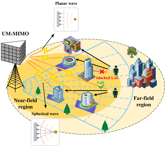
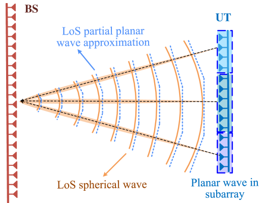
Consider an ILSC scenario in mmWave UM-MIMO systems as shown in Fig. 1, where a BS serves UTs in TDD mode. The BS and UTs are all equipped with a uniform linear array (ULA)111If uniform planar array is considered, the dimensionality of the parameters becomes too large to run the simulation. Therefore, without changing the core of the problem, we have made a relatively idealized treatment of the practical problem in order to gain an understanding of the essential problem of HFBS effect in channel estimation and localization, and to gain corresponding insights., and comprise antennas and RF chains. To reduce the hardware costs and power consumption of UM-MIMO, the BS and UTs all employ hybrid beamforming architecture with a much smaller number of RF chains than that of antennas, i.e., . Moreover, the cyclic prefix orthogonal frequency division multiplexing (CP-OFDM) with subcarriers is adopted to combat the frequency selective fading of the broadband mmWave channels.
II-A Uplink Reference Signal Transmission
At this stage, multiple UTs transmit mutually orthogonal reference signals in the consecutive time slots in the uplink to acquire CSI. For a specific UT, in order to estimate the -th subcarrier’s CSI, the received baseband signal at the BS in the -th time slot can be formulated as
| (1) |
where and . In (II-A), represents the BS’s receive combining matrix , in which and are the analog and digital receive combining matrices respectively, is the number of independent received signal streams on each subcarrier. By activating only one RF chain in one time slot for UT, the RF reference signal vector transmitted by the UT can be denoted as . is the total uplink transmit power, while is the baseband reference signal with . In addition, stands for the corresponding uplink frequency-domain channel matrix, whose modeling approach will be detailed in Sec. II-B, and is the complex additive white Gaussian noise (AWGN) with the covariance matrix , i.e., . Due to the constant modulus constraint of the adopted fully-connected RF phase shift network at the BS and UT, the uplink transmit and combining matrices can be expressed as and respectively, where and denote the phase value connecting the -th antenna and the -th RF chain, respectively.
| (2) |
II-B Channel Model with HFBS Effect
Considering the channel reciprocity in TDD systems, we focus on the formulation of the uplink channel matrix next. In an mmWave UM-MIMO system with a hyper-scale antenna aperture and ultra-wide bandwidth, the channel exhibits an intrinsic HFBS effect. Our study specifically targets scenarios that are representative of indoor and short-range localization and communication environments, rather than urban macro-cell (UMa) environments. In these indoor settings, both near-field and far-field effects are present, along with significant beam squint effects due to the large antenna aperture and wide bandwidth, which are distinct from the purely far-field propagation considered in UMa scenarios. Under the spherical wavefront assumption, the spatial-frequency domain hybrid near- and far-field channel matrix can be accurately modeled as (2) shown at the top of next page, which is a sum of the contributions of multipath components (MPCs) including one LoS MPC and several non-LoS (NLoS) MPCs reflected by scattering clusters [42]. Particularly, for the LoS component , its -th element can be further written as
| (3) |
where is the large-scale fading gain of the LoS link, represents the wavelength of the -th subcarrier, and denotes the physical distance between the -th antenna element of the BS and the -th antenna element of the UT.
For the -th NLoS component, it can be decomposed into the product of frequency-dependent array manifold of BS and UT sides under the spherical wave assumption, which can be further concretely presented as [25]
| (4) |
Herein, and denote the distance and AoA between the -th scatterer and the reference point of BS’s antenna array, respectively. Without loss of generality, the reference point could be set to the center of the antenna array. More generally, represents the distance between the -th scatterer and the -th element of BS’s antenna array. Under the spherical wave assumption, is a function of both and , i.e., , in which with , and denotes adjacent antenna spacing commonly with half-wavelength. Similarly, can be expressed as
| (5) |
where and denote the distance and AoD between the reference point of UT’s antenna array and the -th scatterer, respectively. Additionally, in (2), and are the large-scale fading gain of the NLoS link and small-scale channel gain corresponding to the -th NLoS component, respectively.
Note that in practical environments, multi-hop paths experience significant path loss, as shown in [43], where each hop results in approximately 6 dB reflection loss and 12 dB transmission loss in a building scatterer scenario. Consequently, these multi-hop signals are treated as noise, having a minimal effect on both communication and sensing capabilities. Therefore, in the modeling presented in this paper, only single-hop NLoS components are considered.
III Uplink Channel State Information Acquisition
This section introduces the uplink CSI acquisition, i.e., the BS estimates the uplink channels based on the pilot signals transmitted by the UTs. Specifically, we first conceive a dedicated frame structure for ILSC and formulate the channel estimation problem as a structured CS problem. Moreover, we conceive a frequency-dependent hybrid-field projection matrix to unveil the inherent sparse pattern of the channels with HFBS effect. Finally, we develop an algorithm that combines AMP with the EM technique to address this CS problem.
III-A Problem Formulation
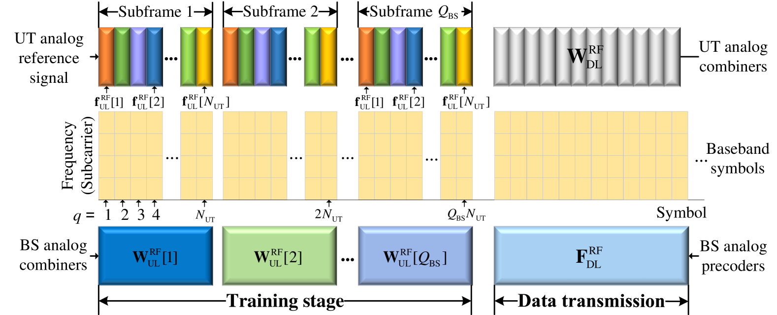
The designed frame structure for ILSC is depicted in Fig. 2. Its time-frequency radio resources can be divided into multiple resource elements to convey both reference signals and payload data. Specifically, the first symbols are allocated for channel training, while the remaining resources are reserved solely for payload data transmission. During the full frame, the discrete Fourier transform (DFT) length of an OFDM symbol is set to . Consequently, the symbol duration of the reference signal becomes , where represents the CP length, and is the system bandwidth. Furthermore, the reference signals in the training stage consists of subframes. Within each subframe, the BS analog receive combiner remains constant, and its phase shift of -th elements for and are uniformly distributed in . Meanwhile, the digital receive combiner at the BS adopts an identity matrix , where . In this setting, UTs transmit orthogonal reference signals in each subframe, which could be designed as a DFT matrix as to meet the prerequisites of constant modulus and orthogonality.
Based on the above assumptions, by collecting for all subframes together (where is the subframe index and is the symbol index in one subframe), the aggregate received signals can be written as
| (6) |
where successively selects every symbol of the same subframes as its columns, and stacks different subframes on top of each another, and denotes the effective measurement length. Besides, , is the stacked baseband reference signal, and stands for the corresponding AWGN for all these subframes. Finally, the received baseband signal in (6) is post-processed by multiplying right-hand, i.e.,
| (7) |
in which is the effective noise term.
III-B Projection Matrix Design
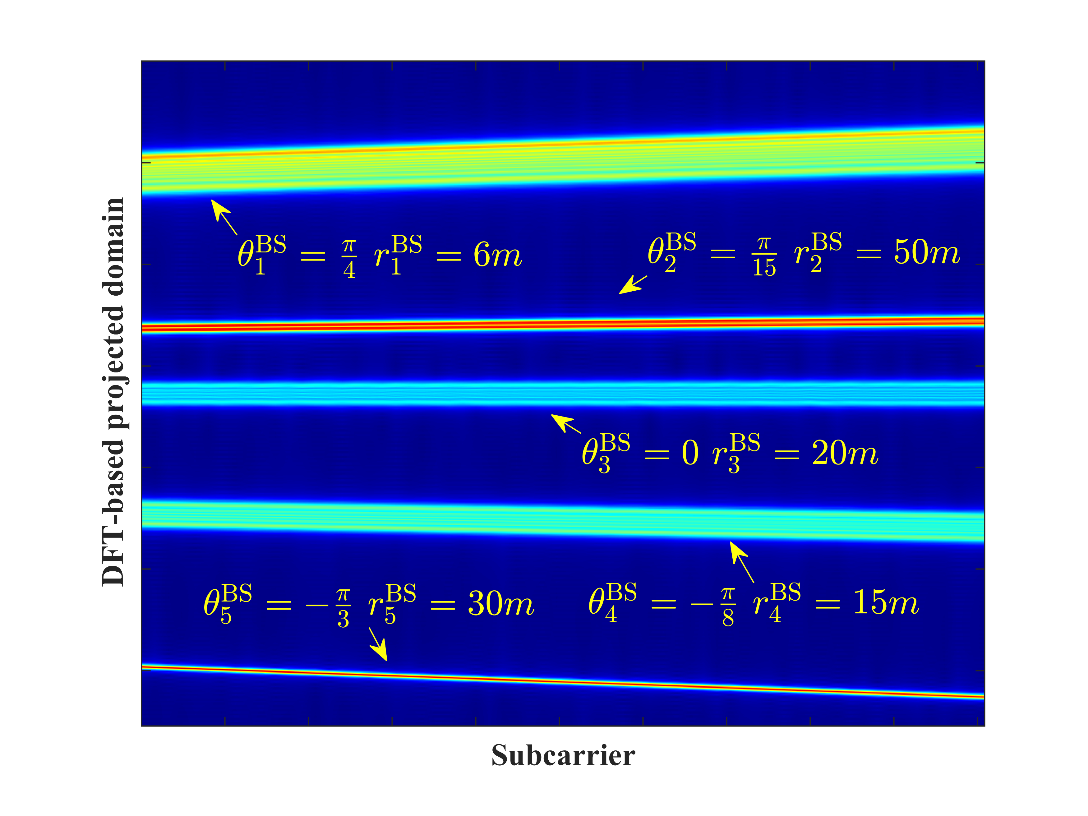
In the case of hybrid far- and near-field propagation effect, the planar wave approximation based projection matrix fails to exactly capture the inherent characteristics of the channel, leading to a degradation in the sparsity of the channels represented in such a projection matrix, as illustrated in Fig. 3(a). To address this issue, a more accurate Fresnel approximation [6] is developed for the distance based on a second-order Taylor expansion as
| (8) |
Based on this approximation, the BS array manifold of each MPC depends on not only its AoD/AoA but also on the distance between the BS and scatterers. To this end, [25, 9] proposed a non-uniform two-dimensional sampling lattice that considers both angles and distances as
| (9a) | |||
| (9b) | |||
where and are the number of grids along the angles and distances, respectively, and is the Rayleigh distance corresponding to the antenna array aperture . Furthermore, is a scaling factor utilized to control the sampling density.
In this way, the projection matrix can be designed as
| (10) |
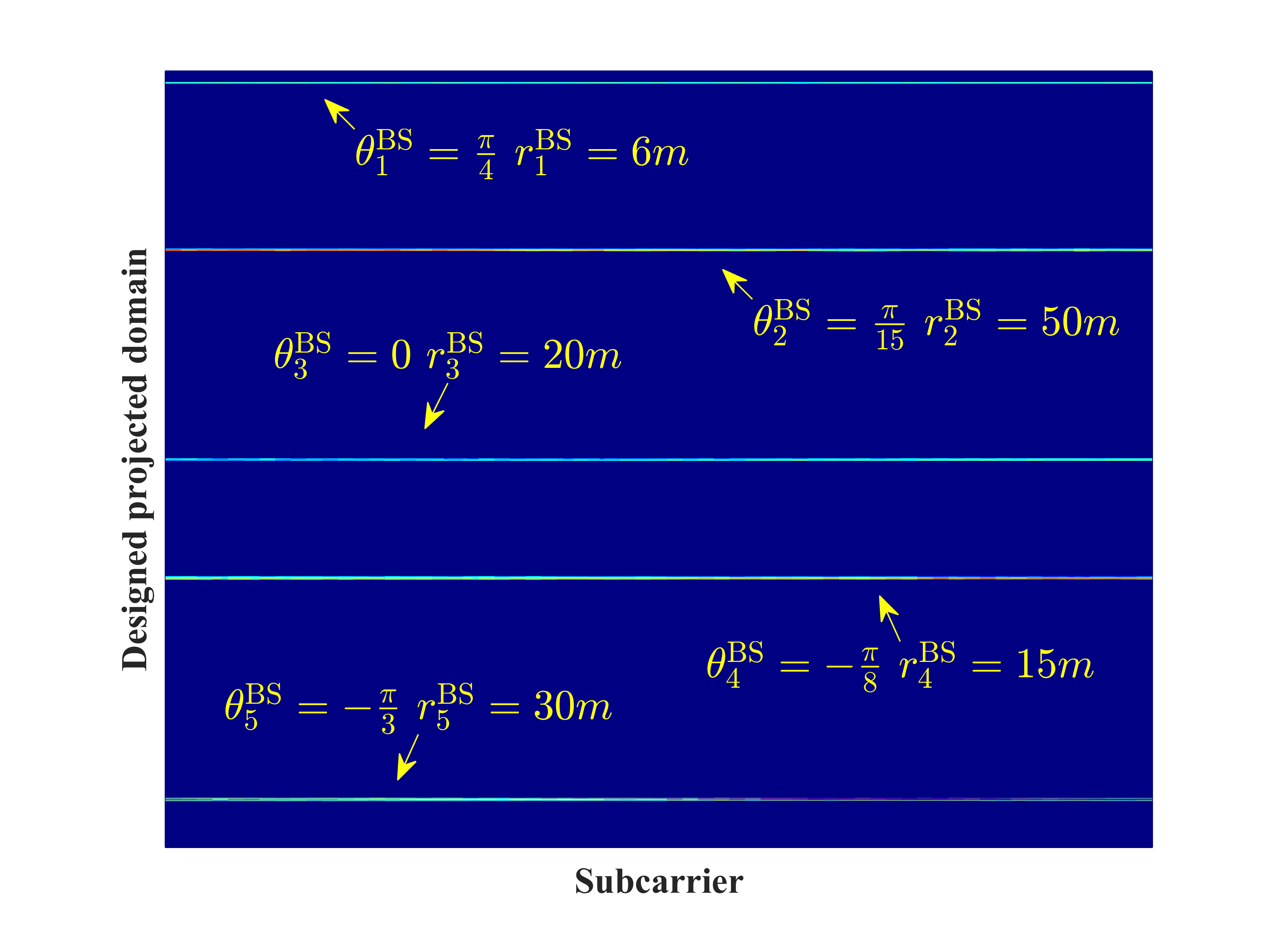
in which the frequency-selective array manifold sampled from the defined 2D lattice forms the -th candidate columns of the projection matrix . It is essential to note that when , , the defined sampling grids match the traditional virtual-angular lattices in the far-field. This alignment indicates that the projection matrix serves as a generalized representation of channels in both far-field and near-field. Furthermore, in contrast to the frequency-flat projection matrix leading to the offset of sparse support sets across different subcarriers [25], the proposed matrix considers the frequency-dependent behavior of the array manifold to ensure an identical support set across the entire frequency spectrum, as illustrated in Fig. 3(b).
As a result, the NLoS components of the HFBS channel can be readily represented in a sparse manner using the defined projection matrix. Furthermore, while the LoS component in (3) cannot be straightforwardly decomposed into the product of two array manifold vectors, it can be approximated as follows using the piece-wise subarray planar wave for UT’s array as depicted in Fig. 3(c)
| (11) |
where indicates the number of subarrays divided for UT’s array, and denote the UT’s array steering vectors of the -th subarray and the BS’s array steering vectors, respecitvely. Under this approximation, the LoS component can be represented sparsely with components as
| (12) |
Therefore, the channel estimation in (7) is equivalent to a structured sparse signal recovery problem
| (13) |
where is the effective sensing matrix and denotes the high-dimensional projected sparse channel matrix.
III-C AMP-EM-Based Channel Estimation
It is well-known that AMP is an efficient iterative Bayesian algorithm for CS problems, which employs low-complexity message passing for approximating the traditional minimum mean square error (MMSE) estimation [44]. For notation brevity, the superscript, subscript, and index have been omitted for and hereinafter, and the different entries of matrix is distinguished by its subscript, e.g., . Starting with the MMSE estimate of , we can obtain its posterior mean as
| (14) |
where denotes the marginal posterior distribution expressed as follows:
| (15) |
(15) requires the high-dimensional integral of joint posterior distribution w.r.t. each variable entry of except . Based on the Bayesian theorem, can be represented as
| (16) |
Under the assumption of AWGN, the above likelihood function obeys complex Gaussian distribution
| (17) |
By following the classic AMP literature [45], we consider the prior distribution of to follow an i.i.d. Bernoulli-Gaussian distribution for effectively capturing its sparsity, i.e.,
| (18) |
where denotes the non-zero probability of , and , are the prior mean and variance of a Gaussian distribution, respectively.
The joint distribution can be represented by a bipartite graph , which consists of variable nodes , factor nodes , and the corresponding edges [46]. This suggests the use of message passing algorithms contributes to rigorous solution of the marginal posterior distribution in (15), and the messages approximation can further reduce the complexity of high-dimensional integral. Therefore, it yields [19]
| (19) |
where indicates the iteration index, and are the message parameters updated at variable nodes as
| (20a) | ||||
| (20b) | ||||
while and are the message parameters updated at factor nodes as
| (21a) | |||
| (21b) | |||
where and are defined in (24). By combining (18) and (19), the marginal posterior distribution can be merged as
| (22) |
where
| (23a) | |||
| (23b) | |||
| (23c) | |||
Then, the posterior mean and variance can be explicitly calculated as
| (24a) | |||
| (24b) | |||
The message switching procedures mentioned in (20)-(24) constitute the fundamental steps of the AMP algorithm. However, several concerns arise when applying the AMP algorithm to practical systems: (a) The hyper-parameters in the prior assumption and the noise variance are often unknown in practice. (b) The column-wise independent solution to the channel estimation problem neglects the common support structure that arises from spatial and frequency correlations. (c) The AMP algorithm is primarily designed for large system limits and typically assumes the use of i.i.d. Gaussian sensing matrices. This assumption is unrealistic for the problem described in (13).
To overcome the first challenge, EM can be exploited to learn the unknown hyper-parameters as [47]
| (25a) | ||||
| (25b) | ||||
where denotes the expectation with respect to the posterior distribution , and its approximation is concluded in (22). By updating one of the elements in (25b) at a time and holding others constant, the learning rules of the hyper-parameters can be summarized as [19]
| (26a) | ||||
| (26b) | ||||
| (26c) | ||||
To further address the second concern aforementioned, it is reasonable to assign a common non-zero probability for each different columns and subcarriers of , which indicates that the learning rule in (26a) and can be refined as
| (27) |
IV Location Sensing
This section leverages the acquired CSI to achieve simultaneous location sensing of the scatterers and UTs without requiring additional radio resources. Specifically, we first extract the targets’ angle and distance information from the spherical electromagnetic wavefront based on the channel estimation results to sense the scatterers’ locations. Then, treating these sensed scatterers as VAs, the UT’s location can be coarsely estimated according to the propagation geometry. To further enhance the sensing performance, we utilize the estimated relative delay of MPCs to refine the UT’s and scatterers’ location through an iterative procedure.
IV-A VAs Location Mapping
Under the spherical wave assumption, the HFBS channel depends not only on the angle of the target, but also on its distance. Therefore, it is feasible to simultaneously derive the angle and distance features of the target from the channel state information. According to the analysis in Section III-B, under ideal conditions, the non-zero support set of sparse channel exactly reflects the approximate LoS components and the NLoS MPCs of the HFBS channel, and their angle and distance parameters are associated with the spatial spatial sampling grid defined in (9). In this way, we can map the location of the center of UT’s subarrays and the scatterers base on the channel estimation results.
One of the premise to achieve location mapping lies on accurate knowleadge about MPCs’ number. To this end, we estimate the effective MPCs’ number based on the minimum description length (MDL) principle, which selects the parametric probability model that fits the dataset best based on the maximum likelihood criterion, so as to estimate the number of signal sources without the need of empirical threshold [50].
Firstly, in order to overcome the rank-deficient problem of covariance matrix caused by coherent multipath signals, the covariance matrix of received pilot signals is calculated with the spatial smoothing technique [49] as
| (28) |
where is the estimated covariance matrix of the original signal, while . By the spectrum decomposition theorem, if there are of the multipath, can be decomposed into
| (29) |
where and are the eigenvalues and eigenvectors of , respectively. Defines a set of parameters for the received signal model, the estimate of can be obtained based on the MDL rule as
| (30) |
where is the joint probability density distribution of the received pilot signals, while . Under the assumption of complex Gaussian distribution, it can be further expressed as (31), which is shown at the top of the next page, where is the estimate of eigenvalue by decomposing the estimated covariance matrix . By calculating the covariance matrix of the received pilot signal on different subcarriers, independent estimation results can be obtained in parallel. Finally, the fusion of different estimation results can be completed by the mode operation.
| (31) |
When the corresponding row energy of the estimated sparse channel is greater than the noise threshold, the MPCs can be considered to exist. Extract the angle and distance parameters of them
| (32) |
where . Unfortunately, due to the finite-resolution sampling lattice, the energy leakage is an inevitable negative effect. As a result, the grids set exhibits a cluster distribution, where truthful peaks are surrouded by a few ghost points. In order to divide clusters before peak identification, K-Means clustering algorithm [52] can be exploited to select the spatial grids subset for the -th effective MPC. In this case, the angle and distance of -th MPC corresponding to the summit of the -th cluster grids can be represented as
| (33) |
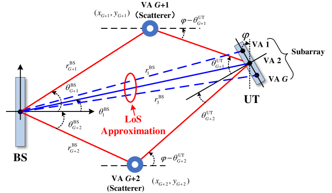
Considering the location sensing geometry illustrated in Fig. 4, where the BS is located at the origin of coordinates, we can coarsely map the position of VAs with the orientation and distances measured above as , where we treat the sensed UT subarray centers and scatterers equally as VAs, and they can contribute to UT location sensing hereinafter. In order to distinguish the sensed UT subarray centers from the scatterers, we adopt the following method: VAs satisfying the array aperture constraint are inferred as UT subarray centers, and their coordinate set , where is the VAs with the maximum energy and thus can be truthfully inferred as LoS components, while is the antenna array aperture of UT. The remains are classified as scatterers and their coordinate set .
IV-B Coarse UT Location Sensing
In order to acquire the UT’s position with the aid of sensed VAs, one of the prerequisites lies in acquiring the orientation between the UT and VAs. For this purpose, motivated by the channel eigenvector decomposition in (2) and LoS approximation in (III-B), and the BS steering vector can be estimated as , thus the angle and distance can be estimated via matching pursuit as
| (34) |
It is noteworthy that since the array aperture of UT is much smaller than that of BS, the Rayleigh distance observed from UT could be relatively small so that the uncertainty of aggravates. In this context, the geometric propagation model used for UT’s location sensing in Fig. 4 can be represented irrespective of as
| (35) |
where is the location of UT to be determined, and is the inclination angle of UT’s array. Furthermore, it can be rewritten with a matrix form as
| (36) |
In view of the non-uniform sampling pattern defined in (9), the further the VAs locate, the sparser the corresponding sampling grid is. If the scatterer falls into a region with sparser spatial sampling grids, the location sensing error for those VAs would aggravate, and their reliability for UT localization would decline. Therefore, one viable solution to the above problem is the weighted least squares (w-LS) method [51], which introduces a weighted matrix assigning higher weights to VAs with smaller sampling interval and lower weights to VAs with larger sampling interval, thereby enhancing the accuracy of the estimation, i.e.,
| (37) |
where and are estimated by replacing the corresponding element with the sensing results in (33) respectively, while can be estimated as . Moreover, the weighted matrix can be expressed as , and denotes the distance parameter of nearest adjacent grid set in (9) corresponding to .
Remark 1
In fact, the above mentioned UT localization method can also be extended to blocked LoS case. In the absence of LoS component, compared with (35), the only difference for location sensing problem lies in the absence of information about LoS orientation , , which does not yet affect its rigorous LS solution when the number of sensed VAs meets .
IV-C Sensing Result Refinement
The aforementioned coarse UT’s location sensing result only depends on the angle and distance information extracted from the spherical wavefront, which applies to both wideband and narrowband sensing tasks in sharp contrast to the traditional TDoA-based methods [51]. On that account, benefiting from the available bandwidth in the broadband mmWave systems, the accurately estimated MPCs’ TDoA information can be further utilized to refine the above location sensing result, whose implementation will be detailed next.
Similar to the angle and distance estimation in (IV-B), the relative delay of the -th multipath is firstly obtained by frequency-domain matching filter as
| (38) |
where represents the frequency-domain channel response parameterized by relative channel delay , while are the frequencies of the first, second and subcarriers, respectively. Considering the different geographical locations of transceivers and the limited clock synchronization accuracy, it is difficult to measure the absolute delay of MPCs, and thus it is more effective to exploit the TDoA of MPCs
| (39) |
In addition, the TDoA of MPCs can also be calculated according to the location sensing results
| (40) |
which is the function of coordinates . Owing to the location sensing errors, there exists difference between the calculated TDoA of MPCs and the real TDoA of MPCs, and thus define the loss function as
| (41) |
Following the maximum likelihood principle, the optimal UT and scatterers coordinates tend to minimize the above loss function, but it is intractable to directly derive its optimal closed-form solution. To this end, a feasible solution is to use gradient descent algorithm iteratively update UT and scatterers coordinates and [9]. Therefore, in the -th iteration, one of the parameters in the coordinates is updated each time, while the other parameters are hold unchanged. For instance, the update of the UT’s coordinate can be represented as
| (42a) | |||
| (42b) | |||
To guarantee the convergence of the loss function, an effective approach is Armijo-Goldstein backtracking line search [55] to determine the update step size and . Besides, the location of scatterers can be updated similar to (42). In this case, with a small number of iterations, the refined coordinates are inclined to converge to the appoximately optimal solution. So far, we have finished the discussion about the proposed location sensing scheme for UM-MIMO systems, and its complete procedures are summarized in Alg. 2.
In summary, our approach enhances localization accuracy by leveraging the TDOA technique with multiple scatterers as virtual anchors. By calculating the time differences of arrival from these scatterers to the user, and incorporating the scatterers’ known positions obtained through Alg. 2, our method refines the localization results. This supplementary use of TDOA, despite the presence of only a single BS, effectively enhances the robustness of the localization in environments with significant multipath effects.
V Hybrid Beamforming Design for Downlink Data Transmission
To fully unleash the potential of UM-MIMO for more efficient data transmission, this section designs a beamforming scheme attempting to mitigate the spectral efficiency degradation caused by HFBS issue.
V-A Analog Codebook Design
For the downlink data transmission stage, the received baseband data at the UT on the -th subcarrier can be formulated as the following problem similar to (II-A) as222It is assumed that the BS serves the different UTs using orthogonal time-frequency resources, and thus the beamforming design is optimized for a single specific UT to disclose the impact of HFBS issue.
| (43) |
Different from the parameters defined in (II-A), represents the BS’s transmit beamforming matrix with the power constraint , in which and are the analog and digital beamforming matrices, respectively, and is the number of simultaneous transmitted data streams. Similarly, denotes the UT’s receive combining matrix , where and are the analog and digital combining matrices, while is the payload data stream. In the data transmission stage, we seek to optimize the precoder and combiner that maximizes the beamforming gain over the whole bandwidth and enhance the spectral efficiency (SE) expressed in (44) shown at the top of the next page, where is the noise covariance matrix after combining.
| (44) |
| (47) |
Overcoming beam squint requires that each RF phase shifter generate different phase shift across different subcarriers to form frequency-dispered beamforming vectors. However, the RF phase shifter can only generate the frequency-independent phase shift, greatly limiting its beamforming ability especially in the presence of beam-squint effect. In this case, traditional analog narrow beams design approach that focus on optimizing for center-frequency suffers from serious performance degradation. Therefore, elaborate design of the analog beams codebook is pivotal to an efficient beamforming scheme for hybrid UM-MIMO systems in the presence of HFBS effect.
Without loss of generality, we assume that the reference frequency for designing the analog phase shifts equals the center frequency . Particularly, in the case of , when the beamforming is designed to focus on the postion for the reference frequency, then , where . In this case, the beamforming gain at the given position on the -th subcarrier can be computed as
| (46) |
By means of Fresnel approximation mentioned in (III-B), (V-A) can be further derived as (47), which is shown at the top of the next page.
Denote the beam-squint position that maximize the beamforming gain on the -th subcarrier as , which can be expressed as [11]
| (48a) | ||||
| (48b) | ||||
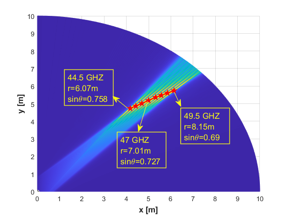
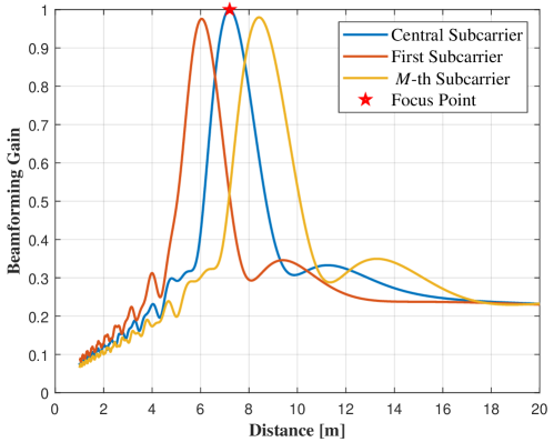
(48) indicates that distinct from the far-field propagation, HFBS effct includes angle squint effect and distance squint effect, respectively. Fig. 5(a) illustrates the beamforming gain distribution with different positions and subcarriers via a heatmap, and the beam-squint trajectory of plotted by a red-star line. To further provide insights into analog beamforming design, we investigate to decouple the variation of beamforming gain along distances or angles, i.e., and , respectively, and disclose the sepreate effects of angle squint and distance squint. Substitute the beam-squint positions derived in (48), and can be expressed as [25]
| (49a) | ||||
| (49b) | ||||
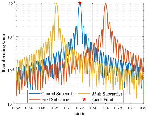
which are displayed in Fig. 5(b) and Fig. 5(c), respectively. On the one hand, it can be observed that the angle squint effect causes the beamforming gain of non-central subcarriers w.r.t. position to fall out of the main lobe and attenuate substantially. On the other hand, the distance squint effect also leads the received energy associated with non-central subcarriers on position to decline by half.
Besides, according to the conclusion derived from (48), to enable the generated beam to focus on the expected location for the -th subcarrier, should meet
| (50a) | ||||
| (50b) | ||||
Therefore, to provide constant beamforming gain as much as possible over the whole bandwidth and maximize SE, one intuitive compromise is to generate beams covering all so that the traditional narrow beams are required to be broadened along both the distance and angle at the reference frequency, with the maximum angle and distance intervals and , respectively.
The generation of beam can employ a subarray based beam aggregation method [29], which divides the antenna array into subarrays and each with elements, and synthesizes the sub-beams generated by different subarrays. Specifically, according to the array signal processing theory, the 3dB beam width of an -elements subarray is and along the normalized angle and distance domains, respectively [56]. In line with the requirements for beam broadening region derived in (50), the number of subarrays should satisfy
| (51a) | |||
| (51b) | |||
And the beamforming vector can be generated subarray-wisely for the -th virtual subarray as
| (52) |
where and . In this problem, in order to maximize the beam gain and improve SE, the beam energy should be focused on UT or the scatterers as much as possible. Therefore, the analog beamforming codebook used to optimize RF phase shifts can be constructed as , which collects all UT’s estimated location, scatterers’ location, and the estimated UT’s subarray center, while , and , , respectively.
V-B Hybrid Beamforming Design with Designed Codebook
Thanks to the mmWave UM-MIMO channel sparsity, the designed analog beamforming codebook is capable of approximately spaning the column space of the unconstrained full-digital beamforming matrix on the m-th subcarrier for , where composes of the first columns of the right singular matrix of [41]. Therefore, the hybrid beamforming design problem under the HFBS effect is equivalent to selecting the best-matched RF beamforming vectors and finding their optimal baseband combination, which can be concretely expressed as
| (53) |
where is a selection matrix used to select beamforming vectors from the codebook for constructing the analog beamformer as . Considering the sparsity of selection matrix , the resulting problem formulation is identical to the optimization problem of sparse signal recovery. Therefore, we straightforwardly exploit the method based on the classic concept of SOMP [41] to obatain the solution of . For the receiver at the UT, the optimal full-digital combiner at each subcarrier is the MMSE combiner in the absence of any hardware restrictions [41]. And the hybrid combiner design at the receiver can be acquired in a similar way to approximate .
VI Simulation Experiments
This section conducts extensive simulation experiments to validate the superiority of our proposed ILSC schemes and compares theri performance with the counterparts in previous literature.
VI-A Simulation Setup
First of all, we present the main system parameters used in simulation experiments in TABLE II 333 Tens up to a hundred GHz will be obtained in THz band for 6G and beyond era[60]. Although the current 5G NR does not have continuous 5 GHz bandwidth, this parameter setting is used to verify the effectiveness of our proposed ILSC scheme, which can be applied to address the HFBS problem in future networks. unless stated otherwise. In addition, the noise power spectrum density at the receivers is , and the power of AWGN is accordingly calculated as . The UT’s and scatterers’ position can be simulated in line with the angle and distance distribution given in TABLE II. For the MPCs resulted from scatterers, we employ the hybrid-field channel model in (2) to generate them. Here, we only count single-hop paths and assume that the small-scale channel gain . The large-scale path loss coefficients of MPCs are determined according to the empirical model provided in Table 7.4.1-1 of [57]. In the uplink, the transmit power of UT ensures the received signal-to-noise-ratio (SNR) to meet . It is important to note that our study focuses on indoor and short-range localization and communication scenarios, rather than UMa environments. Thus, the simulation parameters are chosen to reflect these indoor settings.
| Parameter | Value |
| Number of BS antenna | 512 |
| Number of UT antenna | 32 |
| Number of BS RF chains | 4 |
| Number of UT RF chains | 4 |
| Carrier frequency | |
| System bandwidth | |
| Number of subcarriers | 64 |
| Maximum mumber of MPCs | 6 |
| Scatterer angle distribution | |
| Scatterer distance distribution | |
| UT angle distribution | |
| UT distance distribution | |
| Sampling lattice parameter | |
| AMP damping factor | 0.8 |
| AMP maximum iteration number | 100 |
| Sensing refinement iteration number | 10 |
VI-B Channel Estimation Results
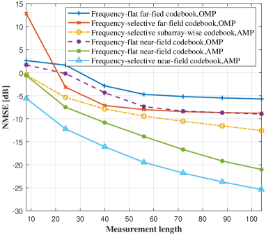
Next, we investigate the performance of the proposed uplink CSI acquistion scheme by evaluating the normalized mean square error (NMSE) between the real channel matrix and its estimation , i.e.,
| (54) |
For comparison, we consider the baseline schemes including
-
(i)
traditional far-field DFT projection matrix based schemes using OMP algorithm [18];
-
(ii)
far-field frequency-selective projection matrix based schemes with beam-squint effect into consideration [27];
-
(iii)
subarray piecewise far-field approximate projection matrix based schemes [23];
-
(iv)
near-field polar-domain projection matrix based schemes using OMP algorithm with the oracle information of MPCs number [25] or AMP algorithm.
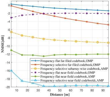
Fig. 6 presents channel estimation performance comparison results versus measurement length and scatterers distance respectively, while in Fig. 6(b), the measurement length is . On the one hand, the performance degradation of traditional far-field sparse channel estimation scheme proves that the channel characteristics in hybrid-field region is different from those in conventional far-field region, and the adopted hybrid-field projection matrix derived based on the Fresnel approximation can better capture its sparsity especially when the scatterers’ or UT’s distance is small. Although dividing the UM-MIMO array into multiple small subarrays and approximate their channel with far-field planar wave is a feasible solution, we still observe that its performance enhancement is limited as it increases the number of angle parameters that need to be estimated to some extent. On the other hand, the significant performance loss caused by the traditional frequency-flat projection matrices illustrates that the beam-squint effect destroys the common support set property of the channels, while utilizing the proposed frequency-dependent projection can address this issue. Moreover, the adopted AMP-EM algorithm shows evident superiority over OMP algorithm since it better exploits the statistical prior information of HFBS channel and AWGN, and can also learn the information of MPCs’ number adaptively.
| Figure 7(a) | Figure 7(b) | |||
| [dB] | [dB] | [dB] | [dB] | |
| Scatterers localization | -11.2081 | -5.6610 | -10.4287 | 2.3688 |
| LoS-only localization | -9.6738 | 4.1412 | -5.4379 | 6.5823 |
| VAs-aided localization | -9.3817 | -1.8237 | -16.5758 | 4.8653 |
| Refined Localization | -9.6900 | -16.9680 | -17.6700 | -22.4413 |
VI-C Location Sensing Results
To evaluate the performance of location sensing, we adopt the root mean square error (RMSE) of UT’s angle and distance estimation as the criteria, which can be defined as
| (55a) | |||
| (55b) | |||
In addition, we consider the following comparison schemes:
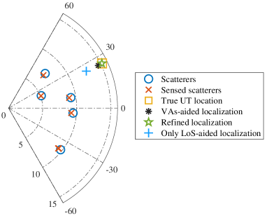
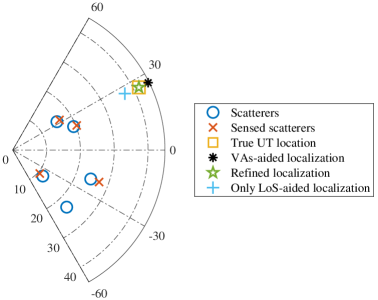
In order to intuitively show the performance of location sensing, we compare the estimated locations of scatterers and UT with their true positions for a single realization with measurement length in Fig. 7. Besides, Table III shows the RMSE performance of the localization for scatterers and UT in Fig. 7, and Table III could also demonstrate the impact of scatterers localization errors on various localization methods. In Fig. 7(a) and Table III, we observe that when UT and scatterers are closer to the BS, all UT and scatterers location can be accurately estimated. By contrast, when UT and scatterers are relatively far away from the BS as shown in Fig. 7(b), the accuracy of scatterers sensing is impaired and missing detection arises due to the non-uniform sampling grid pattern. From Table II, we can conclude that the scatterers localization errors have a significant impact on localization algorithms that rely solely on geometric information. Algorithms utilizing TDoA information, which is our proposed refined localization method, show more resilience to scatterers localization errors. Besides, it can be seen that in Fig. 7(b), there exist 6 MPCs but the estimated number of MPCs is 5. However, its impact on UT location sensing accuracy is insignificant for the VAs-aided localization and refined localization schemes, benefiting from the adopted weighting strategy and high-precision TDoA measurement.
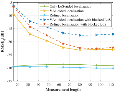
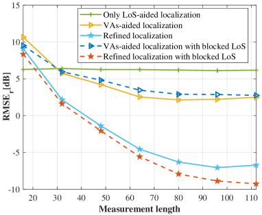
Furthermore, Fig. 8 numerically exhibits the UT sensing performance with the criteria and . It can be observed that with the increase of pilot overhead, the UT location sensing accuracy witnesses sustained improvement until convergence, which indicates that superior channel estimation results contributes to better location sensing performance with a certain range. Owing to ultra-high angular resolution of UM-MIMO array, utilizing LoS information allows high-precision angle estimation, while its distance estimation performance is limited. This is due to the non-uniform spatial sampling lattice, where the grid interval is inversely proportional to the distance. Thus, the straightforward grid mapping with LoS information will inevitably result in worse distance resolution when the target distance increases. To remedy this, joint utilization of VAs can lead to distance estimation enhancement but at a slight cost of angle estimation performance degradation. Particularly worth mentioning is that the aforementioned proposed methods do not depend on the delay information and are thus also suitable for narrowband systems, which offers a new location sensing method for band-limited systems.
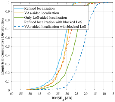
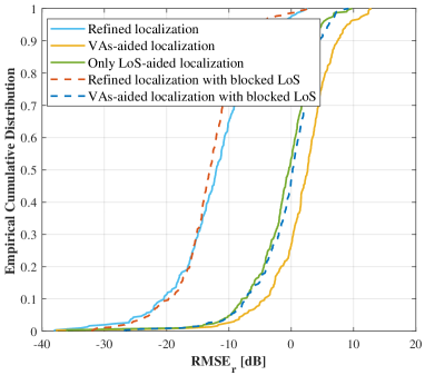
For the broadband systems, the available TDoA information of MPCs can further promote the localization accuracy to the sub-centimeter level. Meanwhile, we investigate the location sensing performance in the absence of LoS link, where the number of NLoS MPCs is set to . We can observe a slight loss in angle estimation accuracy and similar distance estimation performance, which validates the effectiveness of the proposed location sensing method under different channel conditions. On this basis, we further plot the empirical cumulative distribution function (CDF) of and in Fig. 9 with measurement length . Both of them have relatively large variances owing to the non-uniform spatial sampling grid. Take the proposed TDoA-assisted localization method for example, for the best case, and can reach and , respectively. While for the worst case, and degrade to and . Anyway, from the statistical average view, the satisfactory performance can still be achieved.
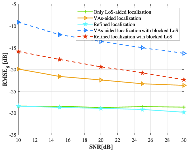
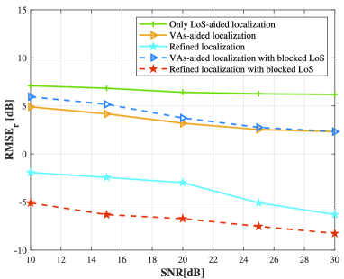
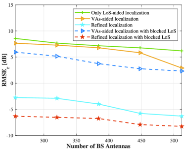
Fig. 10 shows the localization performance comparison against different uplink SNR levels with the number of BS antennas and the number of measurements are set as and , respectively. It can be seen from the figure that the performance of the localization get better as the uplink SNR increases. Besides, the results demonstrate that our proposed refined TDoA-assisted localization method consistently outperforms other approaches across different SNR levels, both in terms of angle and distance estimation, which demonstrates the superiority and the robustness of our methods under various noise conditions.
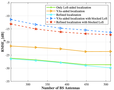
Fig. 11 shows the localization performance comparison against different numbers of BS antennas with the measurement length set as . As evident from both subplots, all localization algorithms demonstrate gradually improving performance as the number of BS antennas increases. The improvement in localization accuracy with more antennas can be attributed to the enhanced spatial resolution and diversity provided by larger antenna arrays, which allow for more precise angle and distance estimation. Besides, methods utilizing TDoA information consistently outperform the method only utilizing the geometric information. The substantial performance improvement demonstrates the importance of incorporating TDoA information in localization problems
VI-D Beamforming Design Results
Finally, we assess the effectiveness of beamforming design for data transmission by the SE criterion defined in (44). The baseline schemes for comparison include
-
(i)
DFT-codebook based spatially sparse precoding scheme [41];
-
(ii)
near-field codebook based beam focusing scheme [58];
-
(iii)
principal component analysis (PCA)-based beamforming scheme [59];
-
(iv)
far-field beam boradening scheme [29];
-
(v)
ideal steering vector (for the center frequency) scheme.
All of the schemes are based on the estimated channel and location sensing results, while the measurement length is set as .
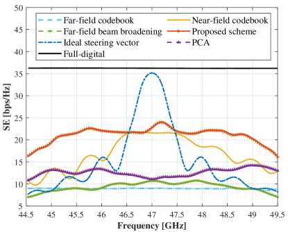
Fig. 12 presents SE results calculated against different subcarriers, where the downlink transmit power is set to . As we can see, the ideal steering vector at the center frequency utilized for analog phase shifts design can ensure approximately optimal beamforming design at the center frequency, but with severe loss at the marginal subcarriers. The traditional DFT codebook-based spatially sparse precoding scheme undergoes the worst performance across the entire frequency band due to its mismatch with the channel’s HFBS feature. The near-field codebook beamforming scheme can remedy the aforementioned drawback but suffers from the problems of the beam-squint effect. Similarly, the far-field beam-broadening scheme handles the probelms caused by the beam-squint effect partially but overlooks the coexisting hybrid-field effect. The proposed scheme jointly optimizes beamforming design by fully considering the HFBS effect and thus achieves the approximately consistent SE performance across the entire bandwidth.
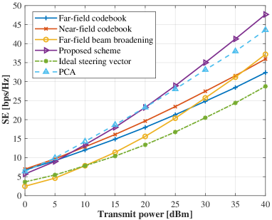
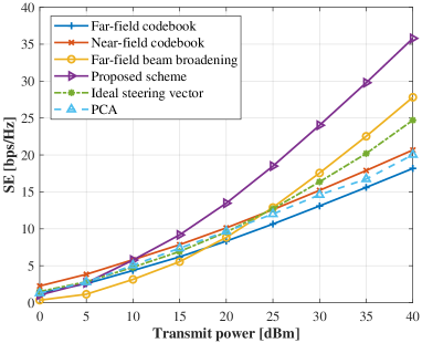
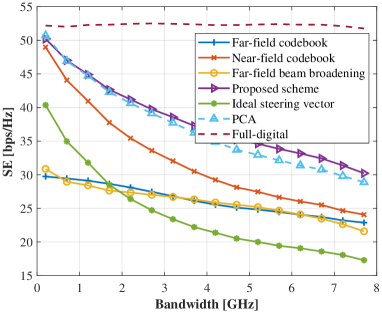
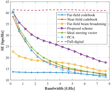
Fig. 13 further compares SE performance with different transmit power in the statistical average view. In the presence of LoS component, the proposed method and the PCA scheme similarly achieve the best performance, while the proposed one maintains the superiority of lower computational complexity without matrix inversion for analog codebook design. The proposed method further expands its advantages in the blocked LoS case and outperforms all other baseline schemes. In Fig. 14, we investigate the SE performance comparison with different bandwidth. When employing a relatively narrow band, all schemes except the far-field assumption based ones harvest satisfactory performance. With the increase of available bandwidth, the performance of all beamforming schemes deteriorates rapidly due to the practical hardware constraint of frequency-independent analog phase shifters. Nevertheless, among them, the proposed one degrades most sluggishly and exhibits best robustness to the HFBS effect.
VII Conclusion
In this paper, we not only overcomed but also exploited the HFBS nature of UM-MIMO systems and investigated a novel ILSC scheme. We commenced with proposing an ILSC signal frame structure consisting of uplink training and data transmission stage. In the uplink training stage, we utilized the designed projection matrix to achieve reliable sparse channel estimation under the HFBS effect, and further sensed the scatterers’ location by extracting the angular and range parameters simultaneously from the spherical electromagnetic wave. Taking the sensed scatterers as VAs, we conceived a w-LS method to coarsely estimate the the UT’s location in line with its propagation geometry. Leveraging the accurately estimated TDoA of MPCs, we further refined the location sensing results to a sub-decimeter level. For the downlink data transmission beamforming design, we utilized the acquired channel and location information, and combined beam broadening and focusing strategy to mitigate the spectral efficiency degradation resulted from HFBS effect, and achieve constant beamforming gain as much as possible over the whole bandwidth and enhance SE. Finally, we carried out simulation experiments to validate the superiority of the proposed ILSC scheme, and the results showed that the proposed schemes outperformed the baseline algorithms in terms of the channel estimation accuracy, location sensing performance, and communication SE.
References
- [1] Qualcomm, Qualcomm Whitepaper Vision, Market Drivers, and Research Directions on the Path to 6G. [Online]. Available: https://www.qualcomm.com/content/dam/qcomm-martech/dm-assets/documents/Qualcomm-Whitepaper-Vision-market-drivers-and-research-directions-on-the-path-to-6G.pdf.
- [2] S. A. Busari et al., “Millimeter-wave massive MIMO communication for future wireless systems: A Survey,” IEEE Commun. Surv. Tutor., vol. 20, no. 2, pp. 836-869, Q2nd. 2018.
- [3] Y. Wang et al., ”Transformer-empowered 6G intelligent networks: From massive MIMO processing to semantic communication,” IEEE Wireless Commun., vol. 30, no. 6, pp. 127-135, Dec. 2023.
- [4] Z. Wang et al., “Extremely large-scale MIMO: Fundamentals, challenges, solutions, and future directions,” IEEE Wireless Commun., early access, Apr. 10, 2023, doi: 10.1109/MWC.132.2200443.
- [5] Z. Wan et al., “Terahertz massive MIMO with holographic reconfigurable intelligent surfaces,” IEEE Trans. Commun., vol. 69, no. 7, pp. 4732-4750, Jul. 2021.
- [6] K. T. Selvan and R. Janaswamy, “Fraunhofer and Fresnel distances: Unified derivation for aperture antennas,” IEEE Antennas Propag. Mag., vol. 59, no. 4, pp. 12–15, Aug. 2017.
- [7] Z. Gao et al., “Integrated sensing and communication with mmWave massive MIMO: A compressed sampling perspective,” IEEE Trans. Wireless Commun., vol. 22, no. 3, pp. 1745-1762, Mar. 2023.
- [8] Y. Chen, R. Li, C. Han, S. Sun, and M. Tao, “Hybrid spherical- and planar-wave channel modeling and estimation for terahertz integrated UM-MIMO and IRS systems,” IEEE Trans. Wireless Commun., vol. 22, no. 12, pp. 9746-9761, Dec. 2023.
- [9] Z. Li, Z. Gao, and T. Li, “Sensing user’s channel and location with terahertz extra-large reconfigurable intelligent surface under hybrid-field beam squint effect,” IEEE J. Sel. Topics Signal Process., vol. 17, no. 4, pp. 893-911, Jul. 2023.
- [10] A. Liao et al., “Terahertz ultra-massive MIMO-based aeronautical communications in space-air-ground integrated networks,” IEEE J. Sel. Areas Commun., vol. 39, no. 6, pp. 1741-1767, Jun. 2021.
- [11] F. Gao, L. Xu, and S. Ma, “Integrated sensing and communications with joint beam-squint and beam-split for mmWave/THz massive MIMO,” IEEE Trans. Commun., vol. 71, no. 5, pp. 2963-2976, May 2023.
- [12] A. Sakhnini, S. De Bast, M. Guenach, A. Bourdoux, H. Sahli, and S. Pollin, “Near-field coherent radar sensing using a massive MIMO communication testbed,” IEEE Trans. Wireless Commun., vol. 21, no. 8, pp. 6256-6270, Aug. 2022.
- [13] J. Yang, C. Wen, J. Xu, H. Que, H. Wei and S. Jin, “Angle-based SLAM on 5G mmWave systems: Design, implementation, and measurement,” IEEE Internet Things J., vol. 10, no. 20, pp. 17755-17771, Oct.15, 2023.
- [14] Z. Wang, X. Mu, and Y. Liu, “Near-field integrated sensing and communications,” IEEE Commun. Lett., vol. 27, no. 8, pp. 2048-2052, Aug. 2023.
- [15] K. Meng, Q. Wu, S. Ma, W. Chen, K. Wang and J. Li, “Throughput maximization for UAV-enabled integrated periodic sensing and communication,” IEEE Trans. Wireless Commun., vol. 22, no. 1, pp. 671-687, Jan. 2023.
- [16] K. Meng, Q. Wu, W. Chen, and D. Li, “Sensing-assisted communication in vehicular networks with intelligent surface,” IEEE Trans. Veh. Technol., vol. 73, no. 1, pp. 876-893, Jan. 2024.
- [17] A. Bayesteh, J. He, Y. Chen, P. Zhu, J. Ma, A. W. Shaban, Z. Yu, Y. Zhang, Z. Zhou, and G. Wang, “Integrated sensing and communication (ISAC)—From concept to practice,” Communications of Huawei Research, pp. 4–25, 2022.
- [18] J. Lee, G. Gil, and Y. Lee, “Channel estimation via orthogonal matching pursuit for hybrid MIMO systems in millimeter wave communications,” IEEE Trans. Commun., vol. 64, no. 6, pp. 2370-2386, Jun. 2016.
- [19] M. Ke, Z. Gao, Y. Wu, X. Gao, and R. Schober, “Compressive sensing based adaptive active user detection and channel estimation: Massive access meets massive MIMO,” IEEE Trans. Signal Process., vol. 68, pp. 764–779, Jan. 2020.
- [20] Z. Gao, S. Liu, Y. Su, Z. Li, and D. Zheng, ”Hybrid knowledge-data driven channel semantic acquisition and beamforming for cell-free massive MIMO,” IEEE J. Sel. Topics Signal Process., vol. 17, no. 5, pp. 964-979, Sept. 2023.
- [21] S. Wu, Z. Ni, X. Meng, and L. Kuang, “Block expectation propagation for downlink channel estimation in massive MIMO systems,” IEEE Commun. Lett., vol. 20, no. 11, pp. 2225–2228, Nov. 2016.
- [22] Z. Gao et al., ”Compressive sensing-based grant-free massive access for 6G massive communication,” IEEE Internet Things J., vol. 11, no. 5, pp. 7411-7435, Mar. 2024.
- [23] Y. Mei et al., “Massive access in extra large-scale MIMO with mixed-ADC over near-field channels,” IEEE Trans Veh. Technol., vol. 72, no. 9, pp. 12373-12378, Sept. 2023.
- [24] Y. Han, S. Jin, C. Wen, and X. Ma, “Channel estimation for extremely large-scale massive MIMO systems,” IEEE Wireless Commun. Lett., vol. 9, no. 5, pp. 633-637, May 2020.
- [25] M. Cui and L. Dai, “Channel estimation for extremely large-scale MIMO: Far-field or near-field?”, IEEE Trans. Commun., vol. 70, no. 4, pp. 2663–2677, Apr. 2022.
- [26] M. Cui and L. Dai, “Near-field wideband channel estimation for extremely large-scale MIMO,” arXiv preprint, arXiv:2212.08401, 2022.
- [27] S. Ma, W. Shen, J. An, and L. Hanzo, “Wideband channel estimation for IRS-aided systems in the face of beam squint,” IEEE Trans Wireless Commun., vol. 20, no. 10, pp. 6240-6253, Oct. 2021.
- [28] K. Wang et al., ”Knowledge and data dual-driven channel estimation and feedback for ultra-massive MIMO systems under hybrid field beam squint effect,” in IEEE Trans. Wireless Commun., early access, 2024.
- [29] F. Gao, B. Wang, C. Xing, J. An, and G. Y. Li, “Wideband beamforming for hybrid massive MIMO terahertz communications,” IEEE J. Sel. Areas Commun., vol. 39, no. 6, pp. 1725-1740, Jun. 2021.
- [30] N. J. Myers and R. W. Heath, “Infocus: A spatial coding technique to mitigate misfocus in near-field LoS beamforming,” IEEE Trans. Wireless Commun., vol. 21, no. 4, pp. 2193-2209, Apr. 2022.
- [31] S. Dwivedi et al., “Positioning in 5G networks,” IEEE Commun. Mag., vol. 59, no. 11, pp. 38-44, Nov. 2021.
- [32] A. Shahmansoori, G. Garcia, G. Destino, G. Seco-Granados, and H. Wymeersch, “Position and orientation estimation through millimeter-wave MIMO in 5G systems,” IEEE Trans. Wireless Commun., vol. 17, no. 3, pp. 1822-1835, Mar. 2018.
- [33] X. Hu, C. Liu, M. Peng and C. Zhong, “IRS-based integrated location sensing and communication for mmWave SIMO systems,” IEEE Trans. Wireless Commun., vol. 22, no. 6, pp. 4132-4145, Jun. 2023.
- [34] Z. Yu, X. Hu, C. Liu, M. Peng and C. Zhong, “Location sensing and beamforming design for IRS-enabled multi-user ISAC systems,” IEEE Trans. Signal Process., vol. 70, pp. 5178-5193, 2022.
- [35] L. Qiao et al., “Sensing user’s activity, channel, and location with near-field extra-large-scale MIMO,” IEEE Trans. Commun., vol. 72, no. 2, pp. 890-906, Feb. 2024.
- [36] Y. Huang and M. Barkat, “Near-field multiple source localization by passive sensor array,” IEEE Trans. Antennas and Propag., vol. 39, no. 7, pp. 968-975, Jul. 1991.
- [37] J. Liang and D. Liu, “Passive localization of mixed near-field and far-field sources using two-stage MUSIC algorithm,” IEEE Trans. Signal Process., vol. 58, no. 1, pp. 108-120, Jan. 2010.
- [38] A. Guerra, F. Guidi, D. Dardari, and P. M. Djurić, “Near-field tracking with large antenna arrays: Fundamental limits and practical algorithms,” IEEE Trans. Signal Process., vol. 69, pp. 5723-5738, Aug. 2021.
- [39] O. Rinchi, A. Elzanaty, and M. Alouini, “Compressive near-field localization for multipath RIS-aided environments,” IEEE Commun. Lett., vol. 26, no. 6, pp. 1268-1272, Jun. 2022.
- [40] K. Meng, et al., “Cooperative ISAC Networks: Opportunities and Challenges,” arXiv preprint arXiv:2405.06305, May 2024.
- [41] O. Ayach, S. Rajagopal, S. Abu-Surra, Z. Pi, and R. W. Heath, “Spatially sparse precoding in millimeter wave MIMO systems,” IEEE Trans Wireless Commun., vol. 13, no. 3, pp. 1499-1513, Mar. 2014.
- [42] Y. Liu, Z. Wang, J. Xu, C. Ouyang, X. Mu, and R. Schober, “Near-field communications: A tutorial review,” IEEE Open J. Commun. Soc., vol. 4, pp. 1999-2049, Aug. 2023.
- [43] K. R. Schaubach, N. J. Davis, and T. S. Rappaport, ”A ray tracing method for predicting path loss and delay spread in microcellular environments,” in Proc. Veh. Technol. Soc. 42nd VTS Conf. Front. Technol., Denver, CO, USA, 1992, vol. 2, pp. 932-935.
- [44] D. Donoho, A. Maleki, and A.Montanari, “Message passing algorithms for compressed sensing: I. motivation and construction,” in Proc. Inf. Theory Workshop, Jan. 2010, pp. 1–5.
- [45] X. Meng et al., “Efficient recovery of structured sparse signals via approximate message passing with structured spike and slab prior,” IEEE China Commun., vol. 15, no. 6, pp. 1–17, Jun. 2018.
- [46] F. R. Kschischang, B. J. Frey, and H. A. Loeliger, “Factor graph and the sum-product algorithm,” IEEE Trans. Inf. Theory, vol. 47, no. 2, pp. 498–519, Feb. 2001.
- [47] J. Vila and P. Schniter, “Expectation-maximization Gaussian-mixture approximate message passing,” IEEE Trans. Signal Process., vol. 61, no. 19, pp. 4658–4672, Oct. 2013.
- [48] S. Rangan, P. Schniter, A. K. Fletcher and S. Sarkar, ”On the convergence of approximate message passing with arbitrary matrices,” IEEE Trans. on Inf. Theory, vol. 65, no. 9, pp. 5339-5351, Sept. 2019.
- [49] T. Shan, M. Wax and T. Kailath, “On spatial smoothing for direction-of-arrival estimation of coherent signals,” IEEE Trans. Acoust., Speech, Signal Process., vol. 33, no. 4, pp. 806-811, Aug. 1985.
- [50] M. Wax and T. Kailath, “Detection of signals by information theoretic criteria,” IEEE Trans. Acoust., Speech, Signal Process., vol. 33, no. 2, pp. 387-392, Apr. 1985.
- [51] K. Cheung, H. So, W. Ma, and Y. Chan, “Least squares algorithms for time-of-arrival-based mobile location,” IEEE Trans. Signal Process., vol. 52, no. 4, pp. 1121-1130, Apr. 2004.
- [52] T. Kanungo et al., “An efficient k-means clustering algorithm: Analysis and implementation,” IEEE Trans. Pattern Anal. Mach. Intell., vol. 24, no. 7, pp. 881-892, Jul. 2002.
- [53] X. Shao, C. You, W. Ma, X. Chen, and R. Zhang, “Target sensing with intelligent reflecting surface: Architecture and performance,” IEEE J. Sel. Areas Commun., vol. 40, no. 7, pp. 2070-2084, Jul. 2022.
- [54] T. Cai and L. Wang, “Orthogonal matching pursuit for sparse signal recovery with noise,” IEEE Trans. Inf. Theory, vol. 57, no. 7, pp. 4680-4688, Jul. 2011.
- [55] J. Nocedal and S. J. Wright, Numerical Optimization, New York, NY, USA: Springer, 2006, pp. 448–492.
- [56] M. Cui, Z. Wu, Y. Lu, X. Wei, and L. Dai, “Near-field MIMO communications for 6G: Fundamentals, challenges, potentials, and future directions,” IEEE Commun. Mag., vol. 61, no. 1, pp. 40-46, Jan. 2023.
- [57] 3GPP, “Technical specification group radio access network; Study on channel model for frequencies from 0.5 to 100 GHz,” 3rd Generation Partnership Project (3GPP), Technical Report (TR) 38.901, Mar. 2022, version 17.0.0.
- [58] Y. Zhang, X. Wu and C. You, “Fast near-field beam training for extremely large-scale array,” IEEE Wireless Commun. Lett., vol. 11, no. 12, pp. 2625-2629, Dec. 2022.
- [59] Y. Sun et al., “Principal component analysis-based broadband hybrid precoding for millimeter-wave massive MIMO systems,”IEEE Trans. Wireless Commun., vol. 19, no. 10, pp. 6331-6346, Oct. 2020.
- [60] A. Shafie et al., “Terahertz communications for 6G and beyond wireless networks: Challenges, key advancements, and opportunities,” IEEE Netw., pp. 1–8, May 2022.