Integrated Adaptive Control and Reference Governors for Constrained Systems with State-Dependent Uncertainties
Abstract
This paper presents an adaptive reference governor (RG) framework for a linear system with matched nonlinear uncertainties that can depend on both time and states, subject to both state and input constraints. The proposed framework leverages an adaptive controller (AC) that estimates and compensates for the uncertainties, and provides guaranteed transient performance, in terms of uniform bounds on the error between actual states and inputs and those of a nominal (i.e., uncertainty-free) system. The uniform performance bounds provided by the AC are used to tighten the pre-specified state and control constraints. A reference governor is then designed for the nominal system using the tightened constraints, and guarantees robust constraint satisfaction. Moreover, the conservatism introduced by the constraint tightening can be systematically reduced by tuning some parameters within the AC. Compared with existing solutions, the proposed adaptive RG framework can potentially yield less conservative results for constraint enforcement due to the removal of uncertainty propagation along a prediction horizon, and improved tracking performance due to the inherent uncertainty compensation mechanism. Simulation results for a flight control example illustrate the efficacy of the proposed framework.
Index Terms:
Constrained Control; Robust Adaptive control; Uncertain Systems; Reference GovernorI Introduction
There has been a growing interest in developing control methods that can handle state and/or input constraints. Examples of such constraints include actuator magnitude and rate limits, bounds imposed on process variables to ensure safe and efficient system operation, and collision/obstacle avoidance requirements. There are several choices for a control practitioner when dealing with constraints. One choice is to adopt the model predictive control (MPC) framework [1, 2], in which the state and input constraints can be incorporated into the optimization problem for computing the control signals. Another route is to augment a well-designed nominal controller, that already achieves high performance for small signals, with constraint handling capability that protects the system against constraint violations in transients for large signals. The second route is attractive to practitioners who are interested in preserving an existing/legacy controller or are concerned with the computational cost, tuning complexity, stability, robustness, certification issues, and/or other requirements satisfactorily addressed by the existing controller. The reference governor (RG) is an example of the second approach. As its name suggests, RG is an add-on scheme for enforcing pointwise-in-time state and control constraints by modifying the reference command to a well-designed closed-loop system. The RG acts like a pre-filter that, based on the current value of the desired reference command and of the states (measured or estimated) , generates a modified reference command which avoids constraint violations. Since its advent, variants of RGs have been proposed for both linear and nonlinear systems. See the survey paper [3] and references therein. While RG has been extensively studied for systems for which exact dynamic models are available, the design of RG for uncertain systems, i.e., systems with unknown parameters, state-dependent uncertainties, unmodelled dynamics and/or external disturbances, has been less addressed.
I-A Related Work
Robust Approaches: As mentioned in [3], the RG can be straightforwardly modified to handle unmeasured set-bounded disturbances by taking into account all possible realizations of the disturbances when determining the maximal output admissible set [4]. For uncertain systems, various robust or tube MPC schemes have also been proposed [5, 6, 7, 8, 9, 10, 11] and summarized in [12], most of which consider parametric uncertainties and bounded disturbances with only a few exceptions (e.g., [10, 11]) that consider state-dependent uncertainties. However, robust approaches often lead to conservative results when the disturbances are large.
Adaptive and uncertainty compensation based approaches could potentially achieve less conservative results than robust approaches. Along these lines, various adaptive MPC strategies with performance guarantees have been proposed for systems with unknown parameters [13, 14, 15] and state-dependent uncertainties [16, 17]. In particular, [15] uses an adaptive controller [18] to compensate for matched parametric uncertainties so that the uncertain plant behaves close to a nominal model, and uses robust MPC to handle the error between the combined system, consisting of the uncertain plant and the adaptive controller, and the nominal model.
To the best of our knowledge, all of the existing adaptive MPC solutions, including [15]
involve propagation of uncertainties along a prediction horizon. Reference [19] merged a Lyapunov function based RG with a disturbance cancelling controller based on an input observer to achieve non-conservative treatment of uncertainties. Unfortunately, a bound on the rate of change of the disturbance is needed for the design, which is often difficult to obtain when the disturbance is dependent on states. Additionally, input constraints were not considered in that work.
State-dependent uncertainties (SDUs):
If a system is affected by SDUs, and the states are limited to a compact set, it is always possible to bound the SDU with a worst-case value and to apply the robust approaches (e.g., robust or tube MPC [5, 6, 7]) developed for bounded disturbances. However, by accounting for the state dependence, one can improve performance and reduce conservatism, as demonstrated in robust MPC solutions in [20, 11]. Adaptive MPC solutions which account for SDUs have been proposed in [16, 17]. These solutions essentially rely on computing the uncertainty or state bounds along the prediction horizon using the Lipschitz proprieties of SDUs, and solving a robust MPC problem, using the computed bounds.
I-B Contributions
The contributions of this paper are as follows. Firstly, for constrained control under uncertainties, we develop an -RG framework for linear systems with matched nonlinear uncertainties that could depend on both time and states, and with both input and state constraints. Our adaptive robust RG framework leverages an adaptive controller (AC) to estimate and compensate for the uncertainties, and to guarantee uniform bounds on the error between actual states and inputs and those of a nominal (i.e., uncertainty-free) closed-loop system. These uniform bounds characterize tubes in which actual states and control inputs are guaranteed to stay despite the uncertainties. A reference governor designed for the nominal system with constraints tightened using these uniform bounds guarantees robust constraint satisfaction in the presence of uncertainties. Additionally, we show that these uniform bounds on state and input errors, and thus the conservatism induced by constraint tightening can be arbitrarily reduced in theory by tuning the filter bandwidth and estimation sample time parameters of the AC. Secondly, as a separate contribution to adaptive control, we propose a novel scaling technique that allows deriving separate tight uniform bounds on each state and adaptive control input, as opposed to a single bound for all states, or adaptive control inputs in existing AC solutions [18]. The ability to provide such separate tight bounds makes an AC particularly attractive to be integrated with an RG for simultaneous constraint enforcement and improved trajectory tracking. Thirdly, we validate the efficacy of the proposed -RG framework on a flight control example and we compare it with both baseline and robust RG solutions in simulations.
Compared to existing literature, in particular, robust/adaptive MPC, -RG has the following novel aspects:
-
•
Thanks to the uncertainty compensation and transient performance guarantees available for the AC, -RG, (under suitable assumptions,) does not require uncertainty propagation along the prediction horizon. This uncertainty propagation is generally required in all existing robust and adaptive MPC approaches, and incurs conservatism, which is avoided by -RG.
- •
-
•
Within -RG, the uniform bounds on the state and input errors (used for constraint tightening) and thus the conservatism induced by constraint tightening can be made arbitrarily small, which cannot be achieved by existing methods.
-
•
-RG is able to handle uncertainties that can nonlinearly depend on both time and states. Such a case has not been considered by previous adaptive MPC solutions that are based on uncertainty compensation. For instance, the solution in [15], which also leverages an AC, only treats parametric uncertainties and state constraints.
The paper is structured as follows. Section II formally states the problem. Section III provides an overview of the proposed solution and discusses preliminaries related to RG and AC design. Section IV introduces a scaling technique to derive separate and tight performance bounds for an AC, while Section V presents synthesis and performance analysis of the proposed -RG framework. Section VI includes validation of the proposed -RG framework on a flight control problem in simulations.
Notations: Let , and denote the set of real, non-negative real, and non-negative integer numbers, respectively. and denote the -dimensional real vector space and the set of real by matrices, respectively. and denote the integer sets and , respectively. denotes an identity matrix of size , and is a zero matrix of a compatible dimension. and denote the -norm and -norm of a vector or a matrix, respectively. The - and truncated -norm of a function are defined as and , respectively. The Laplace transform of a function is denoted by . For a vector , denotes the th element of . Given a positive scalar , denotes a high dimensional ball set of radius and centered at the origin, while its dimension can be deduced from the context. For a high-dimensional set , denotes the interior of and denotes the projection of onto the th coordinate. For given sets , is the Minkowski set sum and is the Pontryagin set difference.
II Problem statement
Consider an uncertain linear system represented by
| (1) |
where , and are the state, input and output vectors, respectively, is the initial state vector, denotes the uncertainty that can depend on both time and states, and and are matrices of compatible dimensions. We want to design a control law for such that the output vector tracks a reference signal while satisfying the specified state and control constraints:
| (2) |
where and are pre-specified convex and compact sets with in the interior. Note that 2 can also represent constraints on some of the states and/or inputs.
Suppose a baseline controller is available and achieves desired performance for the nominal (i.e., uncertainty-free) system given a small desired reference command to track. To enforce state and input constraints 2 for the nominal system with larger signals, one can simply leverage the conventional RG, which will generate a modified reference command based on . In such a case, the baseline controller can be selected as
| (3) |
where and are feedback and feedforward gains. For both improved tracking performance and constraint enforcement in the presence of the uncertainty , we leverage an AC. To this end, we adopt a compositional control law:
| (4) |
where is the vector of the adaptive control inputs designed to cancel . With 3, the uncertain system 1 can be rewritten as
| (5) |
where is a Hurwitz matrix and .
The problem to be tackled can be stated as follows: Given an uncertain system 1, a baseline controller 3 and a desired reference signal , design a RG (for determining ) and the AC for such that the output signal tracks whenever possible, while the state and input constraints 2 are satisfied. We make the following assumption on the uncertainty.
Assumption 1.
Given a compact set , there exist known positive constants , and () such that for any and , the following inequalities hold for each :
| (6a) | ||||
| (6b) | ||||
where denotes the th element of .
Remark 1.
Assumption 1 indicates that in the compact set , is Lipschitz continuous with respect to with a known Lipschitz constant , has a bounded rate of variation with respect to , and is uniformly bounded by a constant .
In fact, given the local Lipschitz constant and the bounded rate of variation , a uniform bound for in can always be derived if the bound on for an arbitrary in and any is known. For instance, assuming we know , from 6a, we have that , which immediately leads to , for any and . In practice, some prior knowledge about the uncertainty (e.g., depends on only a few instead of all states) may be leveraged to obtain a tighter bound than the preceding one, derived using the Lipschitz continuity and triangular inequalities. This motivates the assumption on the uniform bound in 6b.
Remark 2.
Our choice of making assumptions on instead of on as in 8 facilitates deriving an individual bound on each state and on each adaptive input (see Section IV for details).
Remark 3.
In principle, given the uniform bound on in 7b obtained from Assumption 1, constraints can be enforced via robust RG or robust MPC approaches that handle bounded disturbances, as discussed in Section I-A. However, when this bound is large, robust approaches can yield overly conservative performance.
III Overview and Preliminaries
In this section, we first present an overview of the proposed -RG framework and then introduce some preliminary results that provides a foundation for the -RG framework.
III-A Overview of the -RG Framework
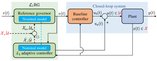
Figure 1 depicts the proposed -RG framework. As shown in Fig. 1, -RG is comprised of two integrated components. The first one is an AC designed to compensate for the uncertainty and to guarantee uniform bounds on the errors between actual states and inputs, and those of the nominal closed-loop system:
| (9a) | ||||
| (9b) | ||||
The second component is a RG designed for the nominal system 9a with tightened constraints computed using the uniform bounds guaranteed by the AC.
More formally, we will design the AC to ensure
| (10) |
where and are the vectors of states and of the total control inputs of the closed-loop system 5:
| (11) |
where is given by 4 and by 9b, and and are some pre-computed hyperrectangular sets dependent on the properties of and of the AC. The details will be given in Theorem 3 in Section III-C. Define
| (12) |
Then for robust constraint enforcement, one just needs to design a RG for the nominal system 9 with tightened constraints given by
| (13) |
III-B Reference Governor Design for a Nominal System
We now introduce the RG for the nominal system 9 to enforce the constraints 13. We use the discrete-time RG approach of [3] that uses a discrete-time model:
| (14) |
where , and denotes the vectors of states, of reference command inputs, and of nominal control inputs, respectively, and and are computed from and in 9 assuming a sampling time, . When doing the discretization, we ensure that the discrete-time system 14 has the same states as the continuous-time system at all sampling instants. This can be achieved by using the zero-order hold discretization, since
| (15) |
which indicates that is piecewise constant. The constraints 13 are imposed in discrete-time as
| (16) |
where and are tightened versions of and , respectively, introduced to avoid inter-sample constraint violations, and are defined by
| (17a) | ||||
| (17b) | ||||
while
| (18) |
with denoting the set of all possible reference commands output by the RG.
The following lemma formally guarantees that no inter-sample constraint violations will happen for the continuous-time system 9 when the constraints for the discrete-time system 21 are satisfied at all sampling instants.
Lemma 1.
Proof.
See Section A-A. ∎
Remark 4.
Remark 5.
In case there are no constraints on certain states and/or inputs, one can remove the rows of and defined in 20 corresponding to these states and/or inputs, and adjust the sets , and accordingly.
Similar to most RG schemes, the RG scheme we adopt here computes at each time instant a command such that, if it is constantly applied from the time instant onward, the ensuing output will always satisfy the constraints. More formally, we define the maximal output admissible set [21] as the set of all states and inputs , such that the predicted response from the initial state and with a constant input satisfies the constraints 21, i.e.,
| (22) |
where for system 14 the output prediction is given by
| (23) |
Define as a slightly tightened version of obtained by constraining the command so that the associated steady-state output satisfies constraints with a nonzero (typically small) margin , i.e.,
| (24) |
where Clearly, can be made arbitrarily close to by decreasing . Based on the currently available state at an instant , the RG computes so that
| (25) |
It is proven in [21] that if is Schur, is observable, is compact with in the interior, and is sufficiently small, then the set is finitely determined, i.e., there exists a finite index such that
| (26) |
Moreover, is positively invariant, which means that if and is applied to the system at time , then . Furthermore, if is convex, then is also convex.
Remark 6.
The process of computing involves computing sets for , and checking the condition ; is the minimum for which this condition holds.
The proposed -RG framework can leverage most of existing RG schemes developed for uncertainty-free systems. As an illustration and demonstration in Section VI, we choose the scalar RG introduced in [22, 23]. The scalar RG computes at each time instant a command which is the best approximation of the desired set-point along the line segment connecting and that ensures . More specifically, the scalar RG solves at each discrete time , the following optimization problem:
| (27a) | ||||
| s.t. | (27b) | |||
| (27c) | ||||
where is a scalar adjustable bandwidth parameter and is the modified reference command to be applied to the system. If there is no danger of constraint violation, and so that the RG does not interfere with the desired operation of the system. If would cause a constraint violation, the value of is decreased by the RG. In the extreme case, , , which means that the RG momentarily isolates the system from further variations of the reference command for constraint enforcement. Due to the positive invariance of , always satisfies the constraints, which ensures recursive feasibility under the condition that at a command is known such that . Response properties of the scalar RG, including conditions for the finite-time convergence of to are detailed in [23].
III-C Adaptive Control Design and Uniform Performance Bounds
We now present an AC that guarantees the bounds in (10), without considering the state and control constraints in 2. We first recall some basic definitions and facts from control theory, and introduce some definitions and lemmas.
Definition 1.
[24, Section III.F] For a stable proper MIMO system with input and output , its norm is defined as
| (28) |
The following lemma follows directly from Definition 1.
Lemma 2.
For a stable proper MIMO system with states , inputs and outputs , under zero initial states, i.e., , we have , for any . Furthermore, for any matrix , we have .
A unique feature of an AC is a low-pass filter (with DC gain ) that decouples the estimation loop from the control loop, thereby allowing for arbitrarily fast adaptation without sacrificing the robustness [18]. For simplicity, we can select to be a first-order transfer function matrix
| (29) |
where () is the bandwidth of the filter for the th input channel. We now introduce a few notations that will be used later:
| (30a) | ||||
| (30b) | ||||
where correspond to system 9 and to 1. Also, letting be the state of the system we have . Defining , and further considering that is Hurwitz and is compact, we have according to Lemma 2.
III-C1 adaptive control architecture
For stability guarantees, the filter in (29) needs to ensure that there exists a positive constant and a (small) positive constant such that
| (31a) | ||||
| (31b) | ||||
where
| (32) | ||||
| (33) |
Remark 7.
Remark 8.
A typical AC is comprised of three elements, namely a state predictor, an adaptive law and a low-pass filtered control law. For the system 5, the state predictor is defined by
| (34) |
where is the prediction error, is a Hurwitz matrix, is an arbitrary matrix satisfying and , and and are estimated matched and unmatched disturbances, respectively. The estimates and are updated by the following piecewise-constant adaptive law (similar to that in [18, Section 3.3]):
| (35) |
where is the estimation sampling time and . Finally, the control law is given by
| (36) |
The control law 36 tries to cancel the estimated (matched) uncertainty within the bandwidth of the filter . Additionally, unmatched uncertainty estimate () appears in 34 and 35, although the system dynamics 5 contains only matched uncertainty. This is due to the adoption of the piecewise-constant adaptive law, which may produce nonzero value for . However, a non-zero will not cause an issue either for implementation or for performance guarantee. Additionally, it is possible to prove that for any [25], i.e., the estimated unmatched uncertainty will be close to zero when is small.
III-C2 Uniform performance bounds
We first define some constants:
| (37a) | ||||
| (37b) | ||||
| (37c) | ||||
| (37d) | ||||
where and are defined in 37a, 37b and 37c, respectively. Clearly, for a compact set and are bounded, and . By using Taylor series expansion of , one can show that is bounded, which implies that is bounded. As a result, we have
| (38) |
Further define
| (39) | ||||
| (40) | ||||
| (41) |
where is introduced in 32. Due to 38 and 31b, we can always select a small enough such that
| (42) |
where is defined in 33 and is the pseudo-inverse of .
Following the convention for performance analysis of an AC[18], we introduce the following reference system:
| (43a) | ||||
| (43b) | ||||
Clearly, the control law in the reference system 43 partially cancels the uncertainty within the bandwidth of the filter . Moreover, the control law depends on the true uncertainties and is thus not implementable. The reference system is introduced to help characterize the performance of the adaptive closed-loop system, which will be done in four sequential steps: (i) establishing the bounds on the states and inputs of the reference system (Lemma 3); (ii) quantifying the difference between the states and inputs of the adaptive system and those of the reference system (Theorem 1); (iii) quantifying the difference between the states and inputs of the reference system and those of the nominal system (Lemma 5); (iv) based on the results from (ii) and (iii), quantifying the difference between the states and inputs of the adaptive system and those of the nominal system (Theorem 2).
The proofs of these lemmas and theorems mostly follow the typical AC analysis procedure [18], and are included in appendices for completeness.
For notation brevity, we define:
| (44) |
To provide an overview, Table I summarizes the different (error) systems involved in this section and their related theorems/lemmas, the uniform bounds, the AC parameters and conditions.
| (Error) System | Theorem/Lemma | Uniform Bounds on States and Inputs | AC Parameters | Conditions | |
| 1 | Nominal system 9 | Lemma 2 | N/A | N/A | |
| 2 | Reference system 43 | Lemma 3 | , | 31a | |
| 3 | Diff. b/t reference and adaptive systems | Theorem 1 | 42 and 31a | ||
| 4 | Diff. b/t reference and nominal systems | Lemma 5 | 31a | ||
| 5 | Adaptive system: 5 and the AC | Theorem 1 | , | 42 and 31a | |
| 6 | Diff. b/t adaptive and nominal systems | Theorem 2 | 42 and 31a |
Lemma 3.
For the closed-loop reference system in (43) subject to Assumption 1 and the stability condition in (31a), we have
| (45) | ||||
| (46) |
From 5 and 34, the prediction error dynamics are given by
| (47) |
The following lemma establishes a bound on the prediction error under the assumption that the actual states and adaptive inputs are bounded.
Lemma 4.
Theorem 1.
Remark 9.
For an arbitrarily small , one can always find a small enough such that the constraint 42 is satisfied. According to 40, depends on and , and can be made arbitrarily small by reducing and . Thus, by reducing , both and can be made arbitrarily small, which indicates that the difference between the inputs and states of the adaptive system and those of the reference system can be made arbitrarily small from Theorem 1.
Lemma 5.
Given the reference system (43) and the nominal system (9a), subject to Assumption 1, and the condition 31a, we have
| (51) |
Remark 10.
When the bandwidth of the filter goes to infinity, and thus go to 0. This indicates that the difference between the states of the reference system and those of the nominal system can be made arbitrarily small by increasing the filter bandwidth. However, a high-bandwidth filter allows for high-frequency control signals to enter the system under fast adaptation (corresponding to small ), compromising the robustness. Thus, the filter presents a trade-off between robustness and performance. More details about the role and design of the filter can be found in [18].
From Theorem 1, Lemma 5 and application of the triangle inequality, we can obtain uniform bounds on the error between the actual system 5 and the nominal system 9a, formally stated in the following theorem. The proof is straightforward and thus omitted.
Theorem 2.
Remark 11.
From Remarks 10 and 9, by decreasing and increasing the bandwidth of the filter , one can make (i) the states of the adaptive system arbitrarily close to those of the nominal system; and (ii) the adaptive inputs arbitrarily close to , i.e., the true uncertainty, since is arbitrarily close to when the error between and is arbitrarily small.
IV AC with Separate Bounds for States and Inputs
In Section III-C, we presented an AC that guarantees uniform bounds on the states and adaptive control inputs of the adaptive system with respect to the nominal system, without consideration of the constraints 2. However, as can be seen from Theorem 2, the uniform bound on or is represented by the vector- norm, which always leads to the same bound for all the states, (), or all the adaptive inputs, (). The use of vector- norms may lead to conservative bounds for some specific states or adaptive inputs, making it impossible to satisfy the constraints 2 or leading to significantly tightened constraints for the RG design. To reduce such conservatism, this section will present a scaling technique to derive an individual bound for each () and ().
From Theorem 2, one can see that the bound on (or ) consists of two parts: the first part is (or ) that can be made arbitrarily small by reducing (see Remark 9), while the second part is a bound on (or ). Next, we will derive an individual bound for each (or ).
Derive Separate Bounds for States via Scaling:
For deriving an individual bound for each , we introduce the following coordinate transformations for the reference system 43 and the nominal system 9a for each :
| (55) |
where is a diagonal matrix that satisfies
| (56) |
with denoting the th diagonal element. Under the transformation 55, the reference system 43 is converted to
| (57) |
where
| (58) |
Given a set , define
| (59) |
Similar to 30, for the transformed reference system 57, we have
| (60a) | ||||
| (60b) | ||||
| (60c) | ||||
where are defined in 30. By applying the transformation 55 to the nominal system 9a, we obtain
| (61) |
Letting be the state of the system with , we have . Defining
| (62) |
and further considering Lemma 2, we have . Similar to 31a, for the transformed reference system 57, consider the following condition:
| (63) |
where is defined in 33 and is defined according to 59 and is a positive constant to be determined. Then we have the following result.
Lemma 6.
Consider the reference system (43) subject to Assumption 1, the nominal system 9a, the transformed reference system 57 and transformed nominal system 61 obtained by applying 55 with any satisfying 56. Suppose that 31a holds with some constants and . Then, there exists an constant such that 63 holds with the same . Furthermore,
| (64) | ||||
| (65) |
where we re-define
| (66) |
Proof.
For any satisfying 56 with an arbitrary , we have . Therefore, under the transformation 55, considering 60 and 62 and Lemma 2, we have
| (67a) | ||||
| (67b) | ||||
| (67c) | ||||
| (67d) | ||||
It follows from Lemma 3 that for any , which, together with 55, implies for any , where is defined via 59. Considering 58 and 59, for any compact set , we have
| (68) |
Now suppose that constants and satisfy 31a. Then, due to 68 and 67, with and the same , 63 is satisfied.
Additionally, if 63 holds, by applying Lemma 3 to the transformed reference system 57, we obtain that , implying that for any . Since due to the constraint 56 on , we have 64. Equation 64 is equivalent to for any , with the re-definition of in 66. Following the proof of Lemma 5, one can obtain , where the equality is due to 68. Further considering and due to the constraint 56 on , we have 65. ∎
Remark 12.
Derive Separate Bounds for Adaptive Inputs: From 43b and the structure with 29, we can obtain
| (69) |
Therefore, given a set such that for any , from Assumptions 1 and 2 we get
| (70) |
With the preceding preparations, we are ready to derive an individual bound for () and (), as stated in the following theorem.
Theorem 3.
Consider the uncertain system (5) subject to Assumption 1, the nominal system (9a), and the AC defined via 34, 35 and 36 subject to the conditions 31b and 31a with constants and and the sample time constraint (42). Suppose that for each , 63 holds with a constant for the transformed reference system 57 obtained by applying 55. Then, we have
| (71a) | ||||
| (71b) | ||||
| (71c) | ||||
where
| (72a) | ||||
| (72b) | ||||
with defined in 66, and denoting the element of .
Proof.
Remark 13.
Theorem 3 provides a way to derive an individual bound on , and for each and on for each via coordinate transformations. Additionally, similar to the arguments in Remark 11, by decreasing and increasing the bandwidth of the filter , one can make () arbitrarily small, i.e., making the states of the adaptive system arbitrarily close to those of the nominal system, and make the bounds on and arbitrarily close to the bound on the true uncertainty for , for each .
According to Theorems 2 and 3, the procedure for designing an AC with separate bounds on states and adaptive inputs can be summarized in Algorithm 1.
Remark 14.
One can try different in step 10 of Algorithm 1 and select the one that yields the tightest bound for the th state.
Remark 15.
The conditions 42 and 31 can be quite conservative for some systems, due to the frequent use of inequalities related to the norm (stated in Lemma 2), Lipschitz continuity and matrix/vector norms. As a result, the bandwidth of the filter computed via 31 could be unnecessarily high, while the sample time computed via 42 under a given could be unnecessarily small. Based on our experience, assuming that some bounds () and () satisfying 71 are derived under a specific filter and that satisfy 42 and 31, those bounds will most likely be respected in simulations even if we decrease the bandwidth of by times and/or increase by times.
V -RG: Adaptive Reference Governor for Constrained Control Under Uncertainties
Leveraging the uniform bounds on state and input errors guaranteed by the AC, we now integrate the AC and the RG introduced in Section III-B to synthesize the -RG framework for simultaneously enforcing the constraints 2 and improving the tracking performance.
V-A -RG Design
We first make the following assumption.
Assumption 2.
Remark 16.
Considering 26, 73 implies and (since ) where and , according to 17, are tightened versions of and that are defined in 12. From Remark 13, with a sufficiently high bandwidth for and sufficiently small , one can make arbitrarily close to , and make arbitrarily close to the bound set for the true uncertainty in . Additionally, as mentioned in Remark 4, and are close to and , respectively, when is small. As a result, with a sufficiently high bandwidth for , and sufficiently small and , Assumption 2 roughly states that the initial state stays in , and the constraint set is sufficiently large to ensure enough control authority for tracking an initial reference command and additionally for compensating the uncertainty in .
Under the preceding assumption, the design procedure for -RG is summarized in Algorithm 2. Compared to step 3 of Algorithm 1, we additionally constrain and to stay in for all in step 4 of Algorithm 2. Such constraints can potentially limit the size of uncertainties that need to be compensated and significantly reduce the conservatism of the proposed solution.
We are ready to state the guarantees regarding tracking performance and constraint enforcement provided by -RG.
Theorem 4.
Consider an uncertain system (5) subject to Assumption 1 and the state and control constraints in 2. Suppose that an AC (defined by 36, 35 and 34) and a RG are designed by following Algorithm 2. If Assumption 2 hold, then, under the baseline control law 3 and the -RG consisting of the compositional control law 4, the AC and the RG for computing the reference command according to 15 and 27, we have
| (74) | ||||
| (75) | ||||
| (76) |
where and are the states and outputs of the nominal system 9 under the reference command input , and
| (77) |
Proof.
Equation 73 in Assumption 2 implies (due to ), and . Thus, the reference command produced by 27 ensures and for all , which, due to Lemma 1, implies
| (78) |
Compared to 3, 16 and 20 of Algorithm 1, we restrain and to be subsets of in 4, 9 and 13 of Algorithm 2. As a result, if 74 and
| (79) |
jointly hold, condition 75 holds according to Theorem 3, while 65 holds according to Lemma 6.
We next prove 74 and 79 by contradiction. Assume 74 or 79 do not hold. The initial condition 73 implies that and . As a result, we have , and . Since , and are continuous, there must exist a time instant , such that
| (80a) | ||||
| (80b) | ||||
Now consider the interval . According to Lemma 6, due to 80 and the definitions in 71a and 72a, we have , which, together with 12 and 78, implies
| (81) |
Similarly, according to Theorem 3, due to 80 and the definition in 71, we have , and , for any , which, together with 12 and 78, implies
| (82) |
Both 81 and 82 contradict 80b, which proves 74 and 79. By applying the inference right before 82 again for , we obtain 75, which, together with , leads to 76.∎
VI Simulation Results
We now apply -RG to the longitudinal dynamics of an F-16 aircraft. The model was adapted from [26] with slight modifications to remove the actuator dynamics, in which the state vector consists of the flight path angle, pitch rate and angle of attack, and the control input vector includes the elevator deflection and flaperon deflection. The output vector is , where is the pitch angle; the reference input vector is , where and are the commanded pitch angle and flight path angle, respectively. The system is subject to state and control constraints:
| (83) |
where the state constraint can also be represented as following the convention in 2. Furthermore, we assume
| (84) |
The open-loop dynamics are given by
| (85) |
where is the uncertainty dependent on both time and . The feedback and feedforward gains of the baseline controller 3 are selected to be and . Via simple calculations, we can see that when holds.
VI-A -RG Design
It can be verified that given any set , , , , satisfy Assumption 1. For design of the AC in 36, 35 and 34, we select and parameterize the filter as , where denotes the bandwidth for both input channels. Table II lists the bounds on and theoretically computed by applying Algorithm 2 under different and with and without using the scaling technique in Section IV. When applying the scaling technique, we set for each and , which satisfies 56. Several observations can be made from Table II. First, by increasing the filter bandwidth and decreasing , we are able to obtain a smaller satisfying 42 and achieve tighter bounds for all states and inputs. In fact, if and , then are fairly close to the bounds on and for , respectively, which is consistent with Remark 13. Additionally, with scaling, we could significantly reduce and , the bounds on and , and and , the bounds on and . Moreover, with , we can verify that the condition 63 holds with as long as . As mentioned in Remark 15, the conditions 42 and 31 and the resulting bounds and could be conservative. As a result, a larger reference command can potentially be allowed in a practical implementation while keeping to stay in , as demonstrated in the following simulations.
| W/O scaling | With scaling | W/O scaling | With scaling | |
Following Algorithm 2, we used the bounds , and obtained for the case when and , to tighten the original constraints 83 and then used the tightened constraints to design the RG, for which we chose . Considering that was small, we did not consider inter-sample constraint violations and simply set and instead of 17. For comparisons, we also designed a robust RG (RRG) that treats the uncertainty as a bounded disturbance , where is introduced below 85. RRG design also uses set (defined in 22 for RG design); however, the prediction of the output, which corresponds to for RG design, becomes a set-valued one taking into account all possible realizations of the disturbance (see [3] for details). We additionally designed a standard RG by simply ignoring the uncertainty .
VI-B Simulation Results
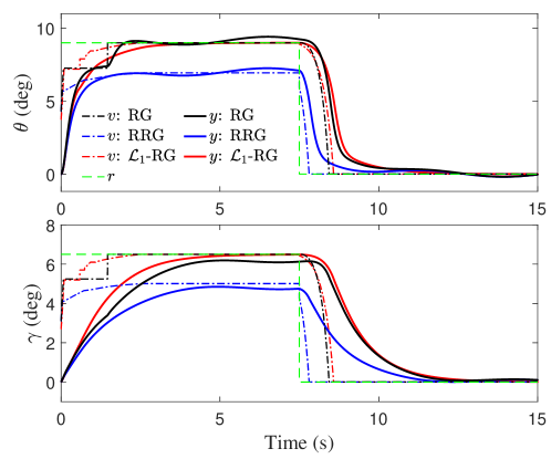
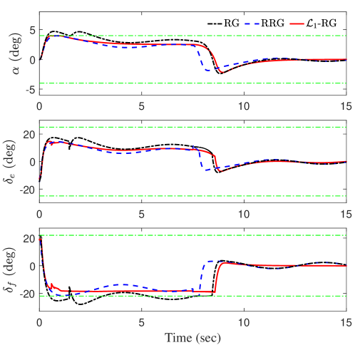
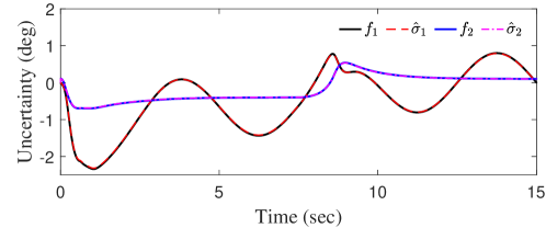
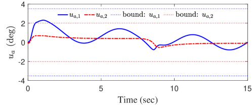
As mentioned in Remark 15, the value of theoretically computed according to 42 is often unnecessarily small. For the subsequent simulations, we simply adopted an estimation sample time of 1 millisecond, i.e., s. As one can see in the subsequent simulation results, all the bounds derived in Section VI-A for and still hold. The reference command was set to be deg for s, and deg for s. The results are shown in Figs. 4, 3 and 2. In terms of constraint enforcement, Fig. 3 shows that both RRG and -RG successfully enforced all the constraints, while violation of the constraints on the state and the input happened under RG. However, from Fig. 2, one can see that the RRG was quite conservative, leading to a large difference between the modified reference and original reference commands and subsequently large tracking errors for both and throughout the simulation. In comparison, the modified reference command under RG reached the original reference command, leading to better tracking performance. Finally, -RG yielded the best tracking performance, driving both and very close to their commanded values at steady state. While noticeable under RG and RRG, the uncertainty-induced swaying in the outputs at steady state was negligible under -RG, thanks to the active compensation of the uncertainty by the AC. From Fig. 4, one can see that the estimation of the uncertainty within the -RG was quite accurate.
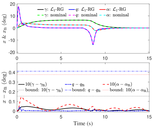
We next check whether the derived uniform bounds on the errors in states, , and on the adaptive inputs, , hold in the simulation. It can be seen from Fig. 5 that the bounds on both and were respected in the simulation and moreover are fairly tight. Figure 6 reveals that all actual states under -RG were fairly close to their nominal counterparts, and moreover, the bound on for each was respected. Note that in Fig. 6 was produced by applying the same reference command yielded by -RG to the nominal system 9.
VII Conclusion
In this paper, we developed -RG, an adaptive reference governor (RG) framework, for control of linear systems with time- and state-dependent uncertainties subject to both state and input constraints. At the core of -RG is an adaptive controller that provides guaranteed uniform bounds on the errors between states and inputs of the uncertain system and those of a nominal (i.e., uncertainty-free) system. With such uniform error bounds for constraint tightening, a RG designed for the nominal system with tightened constraints guarantees the satisfaction of the original constraints by the actual states and inputs. Simulation results validate the efficacy and advantages of the proposed approach.
References
- [1] E. F. Camacho and C. B. Alba, Model predictive control. Springer Science & Business Media, 2013.
- [2] J. B. Rawlings, D. Q. Mayne, and M. M. Diehl, Model Predictive Control: Theory, Computation, and Design, 2nd Ed. Nob Hill Publishing, 2020.
- [3] E. Garone, S. Di Cairano, and I. Kolmanovsky, “Reference and command governors for systems with constraints: A survey on theory and applications,” Automatica, vol. 75, pp. 306–328, 2017.
- [4] I. Kolmanovsky and E. G. Gilbert, “Theory and computation of disturbance invariant sets for discrete-time linear systems,” Mathematical Problems in Engineering, vol. 4, no. 4, pp. 317–367, 1998.
- [5] E. C. Kerrigan, Robust constraint satisfaction: Invariant sets and predictive control. PhD thesis, University of Cambridge, 2001.
- [6] W. Langson, I. Chryssochoos, S. Raković, and D. Q. Mayne, “Robust model predictive control using tubes,” Automatica, vol. 40, no. 1, pp. 125–133, 2004.
- [7] S. Rakovic, Robust control of constrained discrete time systems: Characterization and implementation. PhD thesis, University of London, 2005.
- [8] D. Q. Mayne, S. V. Raković, R. Findeisen, and F. Allgöwer, “Robust output feedback model predictive control of constrained linear systems,” Automatica, vol. 42, no. 7, pp. 1217–1222, 2006.
- [9] D. Q. Mayne, E. C. Kerrigan, E. Van Wyk, and P. Falugi, “Tube-based robust nonlinear model predictive control,” International Journal of Robust and Nonlinear Control, vol. 21, no. 11, pp. 1341–1353, 2011.
- [10] J. Köhler, R. Soloperto, M. A. Müller, and F. Allgöwer, “A computationally efficient robust model predictive control framework for uncertain nonlinear systems,” IEEE Transactions on Automatic Control, vol. 66, no. 2, pp. 794–801, 2020.
- [11] B. T. Lopez, J.-J. E. Slotine, and J. P. How, “Dynamic tube MPC for nonlinear systems,” in Proceedings of American Control Conference, pp. 1655–1662, 2019.
- [12] B. Kouvaritakis and M. Cannon, Model Predictive Control: Classical, Robust and Stochastic. Advanced Textbooks in Control and Signal Processing, Springer, London, 2015.
- [13] K. Zhang and Y. Shi, “Adaptive model predictive control for a class of constrained linear systems with parametric uncertainties,” Automatica, vol. 117, p. 108974, 2020.
- [14] V. Adetola, D. DeHaan, and M. Guay, “Adaptive model predictive control for constrained nonlinear systems,” Systems & Control Letters, vol. 58, no. 5, pp. 320–326, 2009.
- [15] K. Pereida, L. Brunke, and A. P. Schoellig, “Robust adaptive model predictive control for guaranteed fast and accurate stabilization in the presence of model errors,” International Journal of Robust and Nonlinear Control, vol. 31, no. 18, pp. 8750–8784, 2021.
- [16] X. Wang, L. Yang, Y. Sun, and K. Deng, “Adaptive model predictive control of nonlinear systems with state-dependent uncertainties,” Int. J. Robust Nonlinear Control, vol. 27, no. 17, pp. 4138–4153, 2017.
- [17] M. Bujarbaruah, S. H. Nair, and F. Borrelli, “A semi-definite programming approach to robust adaptive MPC under state dependent uncertainty,” in European Control Conference, pp. 960–965, IEEE, 2020.
- [18] N. Hovakimyan and C. Cao, Adaptive Control Theory: Guaranteed Robustness with Fast Adaptation. Philadelphia, PA: Society for Industrial and Applied Mathematics, 2010.
- [19] T. Polóni, U. Kalabić, K. McDonough, and I. Kolmanovsky, “Disturbance canceling control based on simple input observers with constraint enforcement for aerospace applications,” in IEEE Conference on Control Applications, pp. 158–165, IEEE, 2014.
- [20] G. Pin, D. M. Raimondo, L. Magni, and T. Parisini, “Robust model predictive control of nonlinear systems with bounded and state-dependent uncertainties,” IEEE Transactions on Automatic Control, vol. 54, no. 7, pp. 1681–1687, 2009.
- [21] E. G. Gilbert and K. T. Tan, “Linear systems with state and control constraints: The theory and application of maximal output admissible sets,” IEEE Transactions on Automatic control, vol. 36, no. 9, pp. 1008–1020, 1991.
- [22] A. Bemporad and E. Mosca, “Nonlinear predictive reference filtering for constrained tracking,” in Proceedings of European Control Conference, pp. 1720–1725, 1995.
- [23] E. G. Gilbert, I. Kolmanovsky, and K. T. Tan, “Discrete-time reference governors and the nonlinear control of systems with state and control constraints,” International Journal of Robust and Nonlinear control, vol. 5, no. 5, pp. 487–504, 1995.
- [24] C. Scherer, P. Gahinet, and M. Chilali, “Multiobjective output-feedback control via LMI optimization,” IEEE Transactions on Automatic Control, vol. 42, no. 7, pp. 896–911, 1997.
- [25] P. Zhao, S. Snyder, N. Hovakimyana, and C. Cao, “Robust adaptive control of linear parameter-varying systems with unmatched uncertainties,” arXiv:2010.04600, 2021.
- [26] K. M. Sobel and E. Y. Shapiro, “A design methodology for pitch pointing flight control systems,” Journal of Guidance, Control, and Dynamics, vol. 8, no. 2, pp. 181–187, 1985.
- [27] A. Lakshmanan, A. Gahlawat, and N. Hovakimyan, “Safe feedback motion planning: A contraction theory and -adaptive control based approach,” in Proceedings of 59th IEEE Conference on Decision and Control (CDC), pp. 1578–1583, 2020.
- [28] P. Zhao, A. Lakshmanan, K. Ackerman, A. Gahlawat, M. Pavone, and N. Hovakimyan, “Tube-certified trajectory tracking for nonlinear systems with robust control contraction metrics,” IEEE Robotics and Automation Letters, pp. 1–1, 2022.
Appendix A Proofs
A-A Proof of Lemma 1
Proof.
Since the continuous-time system 9 has the same states as the discrete-time system 14 at all sampling instants, if 19 holds for 14, then we have
| (86) |
for 9. Next we analyze the behavior of 9 between adjacent sampling instants. Towards this end, consider any for some and . From 9, we have where the third equality is due to the fact that for all . As a result, we have . Thus, we have
| (87a) | ||||
| (87b) | ||||
where defined in 18, while 87b is due to the fact that . Considering 87, 86 and 17, we have and for all . The proof is complete. ∎
A-B Proof of Lemma 3
Proof.
Rewriting the dynamics of the reference system in (43) in the Laplace domain yields
| (88) |
Therefore, from Lemma 2, for any , we have
| (89) |
where is defined in 44. If 45 is not true, since is continuous and , there exists a such that
| (90) |
which implies for any in . Further considering 7b that results from Assumption 1, we have
| (91) |
Plugging the preceding inequality into 89 leads to
| (92) |
which contradicts the condition (31a). Therefore, (45) is true. Equation (46) immediately follows from (45) and 43. ∎
A-C Proof of Lemma 4
Proof.
Due to 48, we have for any in . Further considering 7b that results from Assumption 1, we have
| (93) |
From (47), for any and , we have
| (94) |
Considering the adaptive law (35), the preceding equality implies
| (95) |
Therefore, for any with , we have
| (96) |
where is defined in 37a, and the last inequality is due to 93. Since , we therefore have
| (97) |
Now consider any such that with . From (94) and the adaptive law 35, we have
| (98) |
where () are defined in 37a, 37b and 37c, and the last inequality is partially due to the fact that . Equations 97 and 98 imply (49). ∎
A-D Proof of Theorem 1
Proof.
We first prove 50c and 50d by contradiction. Assume (50c) or (50d) do not hold. Since and , and , , and are all continuous, there must exist an instant such that
| (99) |
while
| (100) |
This implies that at least one of the following equalities hold:
| (101) |
Note that according to Lemma 3 and from 101. Further considering 7a that results from Assumption 1, we have that
| (102) |
The control laws in 36 and 43 indicate
| (103) |
Equation (47) indicates that
| (104) |
Considering (5), 36 and 104, we have
| (105) |
which, together with 88, implies
| (106) |
Therefore, further considering (102) and Lemma 4, we have
The preceding equation, together with 31b, leads to
| (107) |
which, together with the sample time constraint 42, indicates that
| (108) |
On the other hand, it follows from 102, 103, 104 and 108 that
Further considering the definition in 40, we have
| (109) |
Note that 108 and 109 contradict the equalities in 101, which proves 50c and 50d. The bounds in 50a and 50b follow directly from 50c, 50d, 45 and 46 and the definitions of and in 32 and 41. The proof is complete. ∎