Instabilizability Conditions for Continuous-Time Stochastic Systems Under Control Input Constraints
Abstract
In this paper, we investigate constrained control of continuous-time linear stochastic systems. We show that for certain system parameter settings, constrained control policies can never achieve stabilization. Specifically, we explore a class of control policies that are constrained to have a bounded average second moment for Ito-type stochastic differential equations with additive and multiplicative noise. We prove that in certain settings of the system parameters and the bounding constant of the control constraint, divergence of the second moment of the system state is inevitable regardless of the initial state value and regardless of how the control policy is designed.
Stochastic systems, constrained control, linear systems
1 Introduction
Stabilization under control input constraints is an important research problem due to its wide applicability to systems with actuator saturation. The works [1, 2] describe the challenges of this problem and provide comprehensive discussions of the important results. A key result on this problem is an impossibility result: linear deterministic systems with strictly unstable system matrices cannot be globally stabilized if the norm of the control input is constrained to stay below a constant threshold [3, 4].
There is a rapidly growing interest in exploring control input constraints for stochastic systems. For instance, [5, 6, 7, 8] proposed stochastic model predictive controllers with control constraints; [9] and [10] developed reinforcement learning control frameworks with constraints, [11] investigated fuzzy controllers for stochastic systems with actuator saturation. Constrained control of nonlinear stochastic systems was investigated by [12] and [13], and moreover, [14] explored control constraints in stochastic networked control systems.
The work [15] presented an impossibility result for constrained control of discrete-time stochastic systems. It was shown there that if the control input of a strictly unstable discrete-time stochastic system is subject to hard norm-constraints, then the second moment of the state always diverges under nonvanishing and unbounded additive stochastic process noise. A common approach to overcome the difficulties in the stabilization of strictly unstable systems is to consider probabilistic constraints instead of hard deterministic constraints. However, it was shown in [16] that under certain conditions, stabilization of a discrete-time linear stochastic system is impossible even under probabilistic constraints.
The scope of the impossibility results provided in the abovementioned articles covers discrete-time stochastic systems with additive noise. In this paper, we are motivated to expand this scope by addressing two issues. First, we want to know if similar impossibility results can be obtained for continuous-time stochastic systems. Secondly, we want to investigate the effects of both additive and multiplicative noise terms. Handling multiplicative noise terms is important, since such terms can characterize parametric uncertainties in the system (see [17, 18]). As our main contribution, we identify the scenarios where stabilization of a continuous-time stochastic system (with both additive and multiplicative noise) is not possible under probabilistically-constrained control policies. Specifically, we consider control policies that have bounded time-averaged second moments. This class of control policies encapsulate many types of controllers with (probabilistic or deterministic) control constraints. We obtain conditions on the bounding value of the control constraint, under which the second moment of the state diverges regardless of the controller choice and regardless of the initial state value.
Our analysis for the continuous-time systems with additive and multiplicative noise has a few key differences from that for the discrete-time case with additive-only noise provided in [15, 16]. First, in our case, we handle Ito-type stochastic differential equations with state-dependent noise terms characterizing multiplicative Wiener noise. In addition, we develop a form of reverse Gronwall’s inequality to obtain lower bounds on functions with superlinear growth. Through our analysis, we observe that combination of additive and multiplicative noise can make systems harder to stabilize. Even systems that have Hurwitz-stable system matrices can be impossible to stabilize with constrained controllers under the combination of additive and multiplicative noise.
We organize the rest of the paper as follows. In Section 2, we describe the constrained control problem. Then in Sections 3 and 4, we provide our impossibility results for constrained control of continuous-time stochastic systems. Finally, we present numerical examples in Section 5 and conclude the paper in Section 6.
Notation: We denote the Euclidean norm by , the trace operator by , and the maximum eigenvalue of a Hermitian matrix by . We use to represent the unique nonnegative-definite Hermitian square root of a nonnegative-definite Hermitian matrix , satisfying and . The identity matrix in is denoted by . The notations and respectively denote the probability and expectation on a probability space with sample space and -algebra . We consider a continuous-time filtration with for . Throughout the paper denotes the Wiener process. Here, for every , the process is -adapted; , , are independent processes. Moreover, denotes the complex conjugate of a complex number , and denotes its real part. We use to denote the complex conjugate transpose of a complex matrix , that is, , , . Given a vector , and indices , , we define as .
2 Constrained Control of Continuous-Time Linear Stochastic Systems
Consider the continuous-time linear stochastic system described by the Ito-type stochastic differential equation
| (1) |
for , where is the state with deterministic initial value , is the control input, and moreover, is the Wiener process.
The matrices and are called system and input matrices, respectively. Moreover, and (with ) are noise matrices. The matrix-valued function characterizes the effects of multiplicative noise and it is given by
| (2) |
where , . The matrix in (1) is used for characterizing the effects of additive noise.
Notice that enters in the dynamics as multiplicative noise and enters as additive noise, since .
In this paper, we are interested in a stabilization problem. Since the Wiener process enters in the dynamics in an additive way, the state and its moments cannot converge to regardless of the control input, unless . For this reason, asymptotic stabilization is not possible and a weaker notion of stabilization is needed. In this paper, we consider the bounded second-moment stabilization notion, where the control goal is to achieve .
We consider a stochastic constraint such that the time-averaged nd moment of is bounded by , i.e.,
| (3) |
This constraint is a relaxation of other types of control constraints, i.e., the satisfaction of (3) does not necessarily imply satisfaction of other constraints. Note on the other hand that norm-constraints (e.g., or ), time-averaged norm constraints (e.g., ), as well as first- and second-moment constraints (e.g., or ) all satisfy (3) for certain values of .
Remark 2.1
The structure of (3) is motivated by the networked control problem of a plant with a remotely located controller. In this problem, control commands transmitted from the controller are subject to packet losses, and the plant sets its input to if there is a packet loss (and to otherwise). The actuator at the plant side has a hard constraint requiring for . With randomness involved in packet losses, the plant input actually satisfies (3) with (see Section IV.D of [16] for the specific form of ). Even though the actuator may be powerful ( is large), unstable noisy plants in certain scenarios cannot be stabilized if there are very frequent packet losses, because in such cases is much smaller than , and the controller is unable to provide inputs with sufficient average energy to the plant.
For given , our goal is to find a threshold for , below which stabilization of (1) becomes impossible and the second moment diverges regardless of the controller design.
The following lemmas are used in the derivation of our main result in Section 3. The first lemma is related to the bounding value of the control constraint (3). The second lemma is an extension of Gronwall’s lemma (see, e.g., [19]), where the key condition involves a linear term and the result provides a lower bound instead of an upper bound.
Lemma 2.2
Let , be scalars that satisfy . Then is non-empty.
Proof 2.3.
Let . Since , we have , which implies . Moreover, since , we have . As both and hold, we have , implying that .
Lemma 2.4.
Proof 2.5.
Let for . Since is a continuous function, by fundamental theorem of calculus, we have . Note that (4) implies . Furthermore, since ,
| (6) |
By integrating both left- and far right-hand sides of the inequality (6) over the interval , we get . By using this inequality and , we obtain for , which implies (5), since . Finally, if (4) holds with equality, then for , and thus, (6) holds with equality, which implies that (5) holds with equality.
3 Conditions for Impossibility of Stabilization
In this section, we present our main result, which provides conditions on the control constraint (3), under which the stochastic system (1) is impossible to be stabilized.
Theorem 3.1.
Proof 3.2.
Let . As a first step, we will show Let . It follows from Ito formula (see Section 4.2 of [20]) that
| (11) |
where , , denote the columns of matrix . Under an -adapted control policy, is -adapted. Thus, by Theorem 3.2.1 of [20], we have and . As a result, it follows from (11) that
| (12) |
for . Next, we change the order of expectation and integration in (12) by using Fubini’s theorem [21] and obtain
| (13) |
In what follows, we use (13) to show , separately for two cases: and .
First, consider the case where . In this case, we have , and hence . Furthermore, (7) implies . As a consequence, we obtain from (13) that for all . Therefore, we can use Lemma 2.4 with , , , and to obtain
| (14) |
Notice that is positive, and hence, . Moreover, is positive by the assumption (8). As a result, (14) implies .
Next, we will show that holds also for the case where . For this case let and . By Lemma 2.2, we have .
Now let and define . The scalars and are well-defined since . Moreover, since is a nonnegative-definite Hermitian matrix, we have for any . Using this inequality with , we get
which implies
| (15) |
It then follows from (13) together with and (15) that
| (16) |
Since , we have . Thus, by using with (16), we obtain
| (17) |
Now, since the control policy satisfies (3), we have , and hence, it follows from (17) that
| (18) |
Let , , , and . By definition of , we have , which implies . This inequality and imply . Thus, by Lemma 2.4, we obtain
| (19) |
Since is a nonnegative-definite function, we have . Next, we show . By definition of , we have . Noting that , this inequality implies . Thus, . Now, since , , and hold, (19) implies .
Finally, since (i.e., ), the nonnegative-definite Hermitian matrix has at least one eigenvalue strictly larger than . Thus, . Consequently, implies for . Hence, (10) follows from .
Theorem 3.1 provides sufficient conditions under which the system (1) is instabilizable and the second moment of the state diverges regardless of the controller design and the initial state value. Condition (7) in Theorem 3.1 quantifies the instability of the uncontrolled () system, and the term in (8) represents the effect of additive noise characterized with the matrix . If there is no multiplicative noise (i.e., for ), then (7) requires to be strictly unstable. On the other hand, when there is multiplicative noise, (7) may hold even if is Hurwitz-stable. Notice also that is a nonnegative-definite matrix and it may have as an eigenvalue. This property is essential in our analysis, since it allows us to deal with the cases where some of the states are diverging, while the others are stable.
Theorem 3.1 implies that if conditions (7), (8) hold, then it is not possible to stabilize the system by using control inputs with too small average second moments as in (3). The impossibility threshold on the average second moment of control input is characterized in (9). If , then this threshold value becomes infinity indicating that stabilization is impossible regardless of the input constraint. We note that the case represents the situation, where does not have any effect on .
Remark 3.3 (Instability conditions).
The structure of condition (7) is similar to those of stability/instability conditions provided in [22] for stochastic systems with multiplicative noise. In particular, when specialized to linear systems, Corollary 4.7 of [22] yields an instability condition based on existence of a positive-definite matrix and a scalar such that . Notice that for systems with only multiplicative noise, a positive-definite matrix is required to show global instability. In our setting, a nonnegative-definite matrix is sufficient, because there is also additive noise and (8) guarantees that this noise can make the projection of the state on unstable modes of the uncontrolled system take a nonzero value even if the initial state is zero. Moreover, under the condition (9), diverges, which in turn implies divergence of the second moment of the state, as shown in the proof of Theorem 3.1.
Remark 3.4 (Numerical approach).
We note that linear matrix inequalities can be used for checking the conditions of Theorem 3.1. First of all, for a given , condition (7) is linear in . Similarly, (8) is a linear inequality of . Note that (8) also guarantees that . Moreover, the inequality (9) can be transformed into and which are linear in and , for a given . If the abovementioned inequalities are satisfied with , then with any also satisfies them. To restrict the solutions, we can impose an additional constraint . In our numerical method, we iterate over a set of candidate values of and utilize linear matrix inequality solvers (for each value of ) to check the conditions of Theorem 3.1.
Remark 3.5 (Partial constraints).
Theorem 3.1 can be extended to handle partial input constraints. Consider , where is constrained as in (3) and is unconstrained. If (7)–(9) and hold, then it is impossible to achieve stabilization of this modified system. The proof is similar to that of Theorem 3.1, as implies that is not affected by , and hence (11) holds.
3.1 Tightness of the result for scalar systems
Theorem 3.1 provides a tight bound for in (9) for scalar systems with a scalar state and a scalar constrained input.
Consider (1) with scalars and scalar-valued function such that , , and . In this case, conditions (7) and (8) hold with and . Thus, Theorem 3.1 implies that if the control policy satisfies (3) with , then the system is impossible to stabilize regardless of the initial state . This bound is tight, because, as shown in the following result, stability can be achieved when .
Proposition 3.6.
Proof 3.7.
Let and . By Ito formula (Section 4.2 of [20]),
| (20) |
Now, since is an -adapted process, we obtain and , by using Theorem 3.2.1 of [20]. Thus, with , (20) implies . Therefore, for all , we have , where the last inequality follows from . As a consequence, , which implies that stability is achieved. Moreover, we have for all , showing that control input constraint (3) is satisfied with .
Proposition 3.6 handles the case where . With similar analysis, we can also show that if , then stays bounded even without control (i.e., ). Furthermore, if , , then a state-feedback control policy with achieves stabilization, and moreover, for , it guarantees the bound for all . This bound can be made arbitrarily small by choosing small . If , , then the system is uncontrollable and grows unboundedly unless .
3.2 Existence of instability-inducing noise matrices
The following proposition complements Theorem 3.1. It shows that if satisfy (7), then for any and , there exists a noise matrix that satisfies both (8) and (9). Thus, by Theorem 3.1, the system with that noise matrix is impossible to be stabilized under constraint (3).
Proposition 3.8.
Proof 3.9.
By the spectral theorem for Hermitian matrices (see Theorem 2.5.6 of [23]), the nonnegative-definite Hermitian matrix can be written as , where are the eigenvalues of and is a unitary matrix. Let denote the columns of . We have . Since , at least one eigenvalue of is strictly larger than . Let . Now, let denote the th entry of vector . Since , at least one entry of is nonzero. We define . Now let and , where , , are columns of . We let for , and set the entries of as
| (21) |
where . Since for , we have
| (22) |
Moreover, since , it follows from (22) that . By using this inequality and noting that , we obtain from (21) that
| (23) |
which implies (8), as , , , and . If , then the inequality (9) holds directly, as . If , then the inequality (23) implies , which in turn implies (9).
4 Special Setting with Only Additive Noise
In this section, we are interested in a special setting, where in (1). In this setting, the system does not face multiplicative noise and it is only subject to additive noise.
We first present an improvement of the numerical approach presented in Remark 3.4. Then we show that eigenstructure of can be used to obtain new instability conditions that are easier to check compared to Theorem 3.1. The eigenstructure-based analysis was previously considered only for discrete-time systems in [16]. Here, we show that continuous-time systems also allow a similar approach.
4.1 Candidate values of in instability analysis
Remark 3.4 provides a numerical approach for checking instability conditions of Theorem 3.1. This approach is based on iterating over a set of candidate values of and checking the feasibility of certain linear matrix inequalities. In the general case with both additive and multiplicative noise, we do not have prespecified bounds for the candidate value set. However, in the case of only additive noise (, i.e., in (2)), the candidate values of can be restricted to belong to the set , where we define as
| (24) |
with denoting the set of eigenvalues of . It is sufficient to choose the values of from the set , as it is not possible to satisfy (7) with and , as shown in the following proposition. Here, we note that with , , the inequality (7) reduces to .
Proposition 4.1.
Let . For every nonnegative-definite Hermitian matrix , there exists such that and , where is defined in (24).
Proof 4.2.
It follows from Lemma A.1 of [16] that , where is an eigenvalue of and is a generalized eigenvector of that satisfies . Let . We have . Moreover, . Therefore, since .
4.2 Instability conditions based on the eigenstructure of
Even with the improvement discussed in the previous subsection, checking feasibility of the linear matrix inequalities mentioned in Remark 3.4 can be computationally costly. In this subsection, we show that the eigenstructure of the system matrix can be used to derive instability conditions that can be checked numerically efficiently.
Let denote the number of distinct eigenvalues of and let with denote those eigenvalues. Moreover, for every , let represent the geometric multiplicity of the eigenvalue . Eigenvalues of are also the eigenvalues of with the same multiplicities. Thus, for every , there exists number of vectors such that
| (25) |
These vectors are called the left-eigenvectors of associated with the eigenvalue . We remark that if is a complex eigenvalue (i.e., ), then the complex conjugate is also an eigenvalue of , and moreover,
| (26) |
where is the complex conjugate transpose of . In the instability conditions presented below, we use the eigenvalues , and the left-eigenvectors , , . Furthermore, we define
Corollary 4.3.
Proof 4.4.
By (25) and (26), for each , we obtain Since is a nonnegative-definite Hermitian matrix, we have (7) with and . Moreover, by the definition of , we have for . Thus, (8) holds with . Now, since (7) and (8) both hold for each , it follows from Theorem 3.1 by setting that under control policies satisfying (3) with , the second moment of the state diverges. Finally, (27) implies that there exists such that , implying divergence.
5 Numerical Examples
In this section, we illustrate our results on two example continuous-time stochastic systems.
Example 1
Consider the continuous-time stochastic system described by (1) and (2) with
| (34) | |||
| (39) |
where are scalar coefficients. The case with corresponds to the linearized dynamics of the forced Van der Pol oscillator (see Section 5.3.1 of [24]).
In each row of Table 1, we consider a different setting for . Our goal is to obtain ranges of such that the system cannot be stabilized with constrained control policies satisfying (3) with chosen in the given range. To obtain the range for each parameter setting, we apply Theorem 3.1. In addition, when there is no multiplicative noise (i.e., ), we also apply Corollary 4.3.
| Setting # | Applied Result | Range of | ||||
| 1 | Theorem 3.1 | |||||
| 2 | Theorem 3.1 | |||||
| 3 | Theorem 3.1 | |||||
| 4 | Theorem 3.1 | |||||
| 5 | Theorem 3.1 | |||||
| Corollary 4.3 | ||||||
| 6 | Theorem 3.1 | |||||
| Corollary 4.3 |
Setting 1 in Table 1 represents the case where is a Hurwitz-stable matrix. Notice that when is Hurwitz-stable, without multiplicative noise, the second moment of the state of the uncontrolled system would remain bounded. However, as Table 1 indicates, under multiplicative noise (with parameters ), the system is unstable under any constrained control that satisfies (3) with .
Settings 2–6 in Table 1 represent different scenarios where is strictly unstable. In each of those settings, different noise parameters are considered. The main observation is that systems with increased noise levels are harder to stabilize with constrained controllers.
Settings 5 and 6 in Table 1 correspond to the cases where there is no multiplicative noise. In those cases Corollary 4.3 can be applied. Notice that Corollary 4.3 provides smaller ranges for compared to Theorem 3.1. This shows that Corollary 4.3 is conservative. We note that the main advantage of Corollary 4.3 is that its conditions can be checked faster than those of Theorem 3.1.
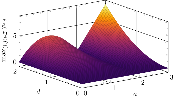
For checking conditions of Corollary 4.3, we can speedily compute in (27). In particular, the computation yields the analytical expression
| (40) |
which is also shown in Fig. 1. Given and , if (i.e., the value is below the surface in Fig. 1), then Corollary 4.3 implies that stabilization of (1) is impossible with a control policy that satisfies (3) with that particular . Notice that is a quadratic function of , and thus, for larger values of , the value of becomes larger. This result is intuitive in the sense that stabilization becomes harder under stronger noise. On the other hand, depends on in a nonlinear nonmonotonic way. It follows from (40) that for , the maximum of is achieved when . For , increases as increases.
Example 2
This system is a noisy version of the uncoupled, linearized, and normalized dynamics that describes a satellite’s motion in the equatorial plane, as provided in [25]. The scalar is the angular velocity of the equatorial orbit along which the system is linearized and the control input is the vector of thrusts applied to the satellite in the equatorial plane. We consider the control input constraint (3) with the average second moment bound .
We check feasibility of the linear matrix inequalities discussed in Remark 3.4 to assess the conditions of Theorem 3.1 for different values of and . When , the conditions of Theorem 3.1 hold for . Thus the system is instabilizable under the control constraint (3) with those values of . On the other hand, with , the corresponding instabilizability range is obtained as .
6 Conclusion
We have investigated the constrained control problem for linear stochastic systems with additive and multiplicative noise terms. We have shown that in certain scenarios, stabilization is impossible to achieve with control policies that have bounded time-averaged second moments. In particular, we have obtained conditions, under which the second moment of the system state diverges regardless of the controller design and regardless of the initial state. Moreover, we have showed the tightness of our results for scalar systems and provided extensions for partially-constrained control policies and additive-only noise settings.
References
- [1] S. Tarbouriech, G. Garcia, J. M. G. da Silva Jr., and I. Queinnec, Stability and stabilization of linear systems with saturating actuators. Springer, 2011.
- [2] A. Saberi, A. A. Stoorvogel, and P. Sannuti, Internal and External Stabilization of Linear Systems with Constraints. Springer, 2012.
- [3] E. D. Sontag, “An algebraic approach to bounded controllability of linear systems,” Int. J. Control, vol. 39, no. 1, pp. 181–188, 1984.
- [4] H. J. Sussmann, E. D. Sontag, and Y. Yang, “A general result on the stabilization of linear systems using bounded controls,” IEEE Trans. Automat. Control, vol. 39, no. 12, pp. 2411–2425, 1994.
- [5] P. Hokayem, E. Cinquemani, D. Chatterjee, F. Ramponi, and J. Lygeros, “Stochastic receding horizon control with output feedback and bounded controls,” Automatica, vol. 48, no. 1, pp. 77–88, 2012.
- [6] M. Korda, R. Gondhalekar, F. Oldewurtel, and C. N. Jones, “Stochastic MPC framework for controlling the average constraint violation,” IEEE Trans. Automat. Control, vol. 59, no. 7, pp. 1706–1721, 2014.
- [7] L. Hewing and M. N. Zeilinger, “Scenario-based probabilistic reachable sets for recursively feasible stochastic model predictive control,” IEEE Control Syst. Lettr., vol. 4, no. 2, pp. 450–455, 2019.
- [8] C. Mark and S. Liu, “Stochastic MPC with distributionally robust chance constraints,” IFAC-PapersOnLine, vol. 53, no. 2, pp. 7136–7141, 2020.
- [9] M. A. Pereira and Z. Wang, “Learning deep stochastic optimal control policies using forward-backward SDEs,” in Robotics: Science and Systems, 2019.
- [10] H. Wang, T. Zariphopoulou, and X. Y. Zhou, “Reinforcement learning in continuous time and space: A stochastic control approach,” J. Mach. Learn. Res., vol. 21, no. 198, pp. 1–34, 2020.
- [11] W.-J. Chang, Y.-W. Lin, Y.-H. Lin, C.-L. Pen, and M.-H. Tsai, “Actuator saturated fuzzy controller design for interval type-2 Takagi-Sugeno fuzzy models with multiplicative noises,” Processes, vol. 9, no. 5, 2021.
- [12] Z. G. Ying and W. Q. Zhu, “A stochastically averaged optimal control strategy for quasi-Hamiltonian systems with actuator saturation,” Automatica, vol. 42, no. 9, pp. 1577–1582, 2006.
- [13] H. Min, S. Xu, B. Zhang, and Q. Ma, “Output-feedback control for stochastic nonlinear systems subject to input saturation and time-varying delay,” IEEE Trans. Automat. Control, vol. 64, no. 1, pp. 359–364, 2018.
- [14] P. K. Mishra, D. Chatterjee, and D. E. Quevedo, “Sparse and constrained stochastic predictive control for networked systems,” Automatica, vol. 87, pp. 40–51, 2018.
- [15] D. Chatterjee, F. Ramponi, P. Hokayem, and J. Lygeros, “On mean square boundedness of stochastic linear systems with bounded controls,” Syst. Control Lettr., vol. 61, pp. 375–380, 2012.
- [16] A. Cetinkaya and M. Kishida, “Impossibility results for constrained control of stochastic systems,” IEEE Trans. Automat. Control, (to appear), 2021. https://doi.org/10.1109/TAC.2021.3059842.
- [17] L. El Ghaoui, “State-feedback control of systems with multiplicative noise via linear matrix inequalities,” Syst. Control Lettr., vol. 24, no. 3, pp. 223–228, 1995.
- [18] R. Khasminskii, Stochastic Stability of Differential Equations. Springer, 2011.
- [19] A. C. King, J. Billingham, and S. R. Otto, Differential Equations: Linear, Nonlinear, Ordinary, Partial. Cambridge University Press, 2003.
- [20] B. Øksendal, Stochastic Differential Equations. Springer, 2005.
- [21] P. Billingsley, Probability and Measure. Wiley, 2012.
- [22] X. Mao, Stochastic Differential Equations and Applications. Elsevier, 2007.
- [23] R. A. Horn and C. R. Johnson, Matrix Analysis. Cambridge University Press, 1985.
- [24] M. Lakshmanan and S. Rajaseekar, Nonlinear Dynamics: Integrability, Chaos and Patterns. Springer, 2012.
- [25] T. E. Fortmann and K. L. Hitz, An Introduction to Linear Control Systems. Marcel Dekker Inc., 1977.