Inspirals from the innermost stable circular orbit of Kerr black holes:
Exact solutions and universal radial flow
Abstract
We present exact solutions of test particle orbits spiralling inward from the innermost stable circular orbit (ISCO) of a Kerr black hole. Our results are valid for any allowed value of the angular momentum -parameter of the Kerr metric. These solutions are of considerable physical interest. In particular, the radial 4-velocity of these orbits is both remarkably simple and, with the radial coordinate scaled by its ISCO value, universal in form, otherwise completely independent of the black hole spin.
I 1. Introduction
Classes of exact orbital solutions in the full Kerr geometry are a known, but under-utilised commodity. Examples include pure circular orbits, radial plunges rev1 , so-called zoom-whirl orbits, and homoclinic orbits, which separate long-lived bound and plunging states LP1 (see LP2 for a useful ‘periodic table’ of different black hole orbits). The study of relativistic test-particle orbits characterised by the energy and angular momentum of a circular orbit, but which are not moving on that orbit, is not new Darwin , but has yet to be astrophysically fully exploited. In this Letter, we analyse an important sub-class of these orbits, and present exact Kerr orbital solutions in a parameter regime of direct physical interest to black hole accretion. While simple in mathematical form, these solutions exhibit revealing features which are important for understanding the accretion process, but have not been discussed before.
One of the most salient features of orbits in Kerr spacetimes is the existence of an innermost stable circular orbit, or ISCO. Exterior to the radial ISCO coordinate , circular orbits are stable and approach their Keplerian velocity behaviour on scales large compared to the horizon radius. Interior to , the angular momentum of a circular orbit increases inward, which means that the orbits are unstable: a tiny perturbation from circular motion will eventually acquire a significant inward radial velocity, even while formally conserving its angular momentum and energy.
Orbits interior to the ISCO are of astrophysical interest because of their direct relevance to black hole accretion theory (e.g., SS ; NT ; PT ). In particular, the question of whether, and if so under what conditions, there can be significant X-ray emission or other observational signatures from matter flowing inward from the ISCO is an active area of current research Wilkins ; Fabian . This problem is generally approached via numerical techniques (e.g., Wilkins ; Potter ), as the assumptions of the classical analytic “viscous” solutions of black hole accretion theory completely breakdown at, and within, the ISCO. The classical viscous disc solution for diverges at the formal ISCO radius NT ; PT , and without a more fundamental understanding of the inflow dynamics, it is not even clear how to frame the underlying equations! With a few notable exceptions Rey ; Wilkins ; Fabian virtually all existing accretion models are artificially cut-off at the ISCO.
In this work we show that there is an overlooked but dramatic simplification of this problem, which provides a clear path forward. The implicit averaging procedure associated with viscous (more accurately, turbulent) disc theory no longer makes sense when the orbits are not circular, but plunging Rey . The need to shed angular momentum vanishes. Instead, in the Kerr geometry angular momentum is simply advected inward with the fluid elements, and thus remains approximately constant and independent of position. What is new here is an explicit solution for the Kerr radial 4-velocity, which determines the surface density directly from mass conservation, and is is both simple and universal in form. This is a key result of this paper. With known, we present exact, closed analytic solutions to the general problem of a test particle starting at at time , and thereafter inspiraling toward the origin. The orbital shape (radial coordinate as a function of azimuthal angle ) is determined entirely in terms of elementary functions. For the Schwarzschild geometry, this orbital shape is exceptionally simple (see eq. [16]). Despite making an appearance in Chandrasekhar’s classic text Chand , it seems to have remained dormant and largely unreferenced in the astrophysical literature. The orbital solutions for more general Kerr geometries, also of astrophysical interest but which seem not to have been discussed in the literature, are best expressed in parameterised form, in a manner analogous to the classical Friedman matter-dominated cosmologies.
II 2. Preliminary analysis
Throughout this work we use geometric units in which both , the speed of light, and , the Newtonian gravitational constant, are set equal to unity. In coordinates , the invariant line element is , where is the usual covariant metric tensor with spacetime indices . (We use the signature convention .) The coordinates are standard Boyer-Lindquist, where is time as measured at infinity, and the other symbols have their usual quasi-spherical interpretation. We shall work exclusively in the Kerr midplane . For black hole mass and angular momentum (both having dimensions of length in our choice of units), the non-vanishing required for our calculation are presented here for convenience (e.g. HEL ):
| (1) |
The 4-velocity vectors are denoted by . Their covariant counterparts , in particular and , have a significance as conserved quantities and are discussed further below. Test particles orbits which spiral inwards, starting at a distant time from a circular orbit at , will preserve their energy and angular momentum. General expressions for the circular angular momentum and energy at radius may be found in HEL :
| (2) | ||||
| (3) |
where
| (4) |
The circular orbits described by eqs. (2) and (3) are not stable at all radii, and it may be shown (e.g., HEL ) that these orbits are stable only when the following condition is satisfied:
| (5) |
which corresponds to . The location of marginal stability corresponds to this expression vanishing:
| (6) |
The form of the second equality will be especially convenient in what follows below.
We label the constants of motion , and use equation (II) to substitute for . The resulting numerators and denominators factor cleanly, leading to an additional simplification:
| (7) | ||||
| (8) |
where in the second equality we have made use of equation (II). Notice that is independent of , apart from the simple implicit dependence.
III 3. Orbital Solutions
III.1 3a. Radial velocity of the ISCO inspiral
As noted earlier, general relativistic dynamics allows for radial motion in orbits whose angular momentum and energy values correspond to an exactly circular orbit. While the governing equation is easily stated
| (9) |
its direct solution is generally a matter of some algebraic complexity. Expressing all non-radial 4-velocities in terms of and , and multiplying through by , we have
| (10) |
Equation (10) is of the form , where is a cubic in which may always be factored:
| (11) |
where and are the general (possibly complex) roots of . ( is, up to an irrelevant factor of , the usual effective potential.)
For an arbitrary circular orbit of radius , both and , and will thus be a double root of the polynomial. For the particular case of a marginally stable circular orbit, there is an additional condition, . Thus, must be a triple root of . The normalisation constant may be found by going back to equation (10) and taking the formal limit . We find
| (12) |
which leads directly to our final equation for :
| (13) |
This may also be verified by a (considerably more lengthy!) direct computation. Note the universality of this remarkable result: there is no -dependence in this expression other than implicitly through . Every Kerr orbit inspiraling from an ISCO is self-similar in its radial motion. As expected, no radial velocity solutions exist for . Despite its generality, simplicity and importance, equation [13] does not appear to have been recognised before in the literature.
The azimuthal component of the intra-ISCO 4-velocity is also simple:
| (14) |
III.2 3b. Schwarzschild orbits
We begin with the Schwarzschild limit . Then , , and . Defining , we find
| (15) |
which immediately integrates to
| (16) |
with the convention that increases from to as goes from to . This is an exact orbital solution for the standard Schwarzschild metric, which is both non-circular and non-radial, extending from to . The reader may verify this by direct substitution into the exact Schwarzschild orbit equation for :
| (17) |
Equation (13) is also easily integrated. This result, moreover, holds for any Kerr ISCO-inspiral orbit, not just for those in the Schwarzschild geometry. With , we find
| (18) |
a universal relationship between proper time and coordinate . It may also be written in parametric form, reminiscent of closed Friedmann cosmologies:
| (19) | ||||
| (20) |
with running from to .
III.3 3c. General solution
The general parameterised azimuthal solution is considerably more complicated. Start with
| (21) |
whence
| (22) |
With substituted from (14) and , this equation has the formal solution
| (23) |
where and may be written in the single compact form:
| (24) |
Both and have poles at the Kerr event horizons, , , at the values given by
| (25) |
and may be evaluated by the Weierstrass substitution
| (26) |
We then find , , where
| (27) | ||||
| (28) |
The two roots of the denominator of the -integrals are
| (29) |
which, from [25], are
| (30) |
After factoring the denominators, the -integrals may be evaluated by partial fraction expansions. Omitting the lengthy but straightforward details, the final result for is
| (31) |
We have defined the constants
| (32) | ||||
| (33) |
This can also be written explicitly as a function of radius:
| (34) |
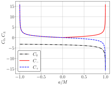
(The arguments of the functions should be inverted for radial coordinates within the horizons .) The -coefficients are plotted as a function of black hole spin in fig. [1]. The Schwarzschild limit and , for which , , is easily verified. An example inspiral trajectory given by equation 34 with is shown in fig. [2]. These solutions have been verified against numerical integration of the geodesic equations.

III.4 3d. Extremal spin limit
The above solution for is ill-defined in the maximal limit, as the two event horizons of the Kerr geometry coincide (), and the partial fraction approach used in solving equation (23) must be revisited. For the solution, the ISCO and event horizons formally coincide in Boyer-Lindquist coordinates. For the orbit is more interesting, and we are able to solve exactly for . We rewrite equation 23 (with , , , and ) as
| (35) |
which becomes
| (36) |
With , we find for :
| (37) |
Inverting equation (36) to solve for (and thus ) is interesting, as it highlights the solutions from all branches of the resulting cubic equation
| (38) |
In fact, there are actually four branches of interest in this problem! Physically this arises from frame dragging, which produces a multi-valued . The three nominal roots of the cubic, , may be written:
| (39) |
with . The fourth branch may be formally identified with the () root, but one must change and into and respectively, as the argument of the exceeds unity for orbits. All four branches are needed, as we now discuss.


The radial solutions for these roots are
| (40) |
with different roots corresponding to different “legs” of the orbit. The path of a test particle inspiralling from the retrograde ISCO of a maximally rotating Kerr black hole is as follows. The particle starts at , with . It spirals inwards towards the event horizon, with increasing , until it crosses the special radius at an angle
| (41) |
whereupon frame-dragging bends the orbit backwards, and the particle begins to corotate with the black hole (Fig. 3). Note that this location is exterior to the ergosphere . During this initial phase the radial coordinate is given by the solution (eq. 39). Beyond this point, the orbit transitions onto the branch, with once again tending towards as the particle approaches the event horizon . Within the event horizon, the orbit is first described by the expression, with , and then the final branch for (Fig 3).
IV 4. Discussion: accretion inside the ISCO
The most important result of this Letter for the modelling of black hole accretion flows is also the simplest, namely equation (13) for , the universal form of the radial 4-velocity for a test particle insprialling from the ISCO radius of a Kerr black hole while retaining its circular energy and angular momentum. This is of great astrophysical interest because the accretion of a steady mass flow in a thin disk is characterised by a constant value of the mass flux (here, is the disk surface density). Here, we have learned that within the ISCO, is generally known a priori and is extremely simple (at least for midplane orbits). A stress term is not needed in this region, and may be ignored since now gravity alone is much more efficient at powering inward flow. By way of contrast, external to the ISCO, to have any systematic radial velocity at all, an enhanced stress is absolutely essential PT ; NT . With this external stress remaining finite at the ISCO itself, the interior and exterior solutions both have vanishingly small velocities at , so that joining these two branches to form a global black hole accretion solution is a natural, and potentially very revealing, next step.
The energetics of the post-ISCO flow is also very important, and becomes much more accessible once the radial velocity is known a priori. The prompt acceleration results in a rapid drop in and therefore the hot internal radiation field will escape more easily. Offsetting this is a radial expansion producing global cooling. This radial expansion is to some extent offset by the vertical compression of the flow near the outer Kerr event horizon, a process which acts to heat the flow. An understanding of the interaction between these competing adiabatic effects, together with self-heating of the disc by its own emission will be needed to account for recent observations that appear to show an additional hot disk component, beyond the expectations of standard theory, in some sources Fabian .
A more precise knowledge of is a very important aid for numerical accretion disk modellers. With a simple form for , and detailed mathematical formulae for and , these results promise to be of great practical utility for numerical code calibration Porth .
Finally, the imaging capabilities now available through the Event Horizon Telescope are on the verge of resolving the flow between the ISCO and event horizon itself Aki . The dynamic properties of the flow in the intra-ISCO region may one day soon be imaged directly. The data from such a study would no doubt provide interesting tests of the models derived here.
We conclude by noting that the mathematical methods used here also work well for other classes of noncircular orbits, which are defined by the energy and angular momentum of a non-ISCO circular orbit, and also for photon orbits. The analytic results of these studies will be fully described in a more lengthy investigation to follow.
Acknowledgements: We thank R. Blandford, K. Clough, P. Feirrera, C. Reynolds and J. Stone for stimulating conversations and helpful advice. This work is partially supported by the Hintze Family Charitable Trust and STFC grant ST/S000488/1.
References
- REFERENCES
- (1) Akiyama, K. et al. 2019, ApJ, 875L, 5E
- (2) Chandrasekhar, S. 1983, Mathematical Theory of Black Holes (Oxford: Clarendon Press)
- (3) Compère G., Liu Y., Long J., 2022, PhRvD, 105, 024075
- (4) Darwin C., 1959, RSPSA, 249, 180
- (5) Fabian A. C., Buisson D. J., Kosec P., Reynolds C. S., Wilkins D. R., Tomsick J. A., Walton D. J., et al., 2020, MNRAS, 493, 5389
- (6) Hobson, M. P., Efstahiou, G., & Lazenby, A. N. 2006, General Relativity: An Introduction for Physicists (Cambridge: Cambridge University Press)
- (7) Levin J., Perez-Giz G., 2009, PhRvD, 79, 124013
- (8) Levin J., Perez-Giz G., 2008, PhRvD, 77, 103005
- (9) Novikov, I. D., Thorne, K. S. 1973, in Black Holes, ed C. DeWitt & B. DeWitt (New York: Gordon & Breach)
- (10) Page D. N., Thorne K. S., 1974, ApJ, 191, 499
- (11) Porth, O. et al. 2019, ApJS, 243, 26P
- (12) Potter, W. J. 2021, MNRAS, 503, 5025
- (13) Reynolds, C. S. Begelman, M. C. 1997, ApJ, 487, 135
- (14) Shakura, N. I., Sunyaev, R. A. 1973, AA, 24, 337
- (15) Wilkins D. R., Reynolds C. S., Fabian A. C., 2020, MNRAS, 493, 5532