OCU-PHYS 552

AP-GR 176

NITEP 125

Inhomogeneous Generalization of Einstein’s Static Universe
with Sasakian Space

Hideki Ishihara [email protected] Satsuki Matsuno [email protected] Department of Mathematics and Physics, Graduate School of Science, Nambu Yoichiro Institute of Theoretical and Experimental Physics (NITEP), Osaka City University, Osaka 558-8585, Japan

Abstract

We construct exact static inhomogeneous solutions to Einstein’s equations with counter flow of particle fluid and a positive cosmological constant by using the Sasaki metrics on three-dimensional spaces. The solutions, which admit an arbitrary function that denotes inhomogeneous number density of particles, are a generalization of Einstein’s static universe. On some examples of explicit solutions, we discuss non-linear density contrast and deviation of the metric functions.

I Introduction

In the general theory of relativity, the investigation of solutions to Einstein’s equations is an important task to understand the structure of the universe. Since it is hard to solve Einstein’s equations, which are non-linear field equations with constraints, almost solutions are found under simplification using isometries.

Among exact solutions with matter sources, one of the most important ones are cosmological solutions of the Friedmann-Lemaître-Robertson-Walker metric, which describe the homogeneous and isotropic universe. Less symmetric solutions are provided by the Lemaître-Tolman-Bondi solutions LTB , where spherically symmetric dust fluid is a source of gravity. It is striking that the solutions admit arbitrary functions. The most known generalization of the Lemaître-Tolman-Bondi solutions are Szekeres’s solutions Szekeres , which admit no geometrical symmetry.

In the solutions noted above, the matter sources are characterized by vanishing vorticity. In contrust, we propose exact solutions to Einstein’s equations with a fluid of particles moving along geodesics with non-vanishing vorticity.

The total spacetimes of the solutions are direct products of time and static three-dimensional space. We take the space homothetic to a three-dimensional Sasakian space Sasaki ; Blair , and construct exact solutions with inhomogeneous fluid with vorticity. The solutions admit an arbitrary function that describes density of the fluid.

II Metric with Sasakian Space

We consider a static metric

\displaystyle ds^{2}

\displaystyle=-dt^{2}+ds_{M}^{2},

(1)

where the metric of the three-dimensional space, $M$ , is given by

\displaystyle ds_{M}^{2}

\displaystyle=a^{2}\left(d\theta^{2}+h(\theta,\phi)^{2}~{}d\phi^{2}\right)+b^{2}(d\psi+f(\theta,\phi)~{}d\phi)^{2}.

(2)

In (2), $a,b$ are constants, $f(\theta,\phi)$ and $h(\theta,\phi)$ are functions to be determined later. The metric (1) admits two unit Killing vectors

\displaystyle\xi_{(t)}=\partial_{t}\quad\mbox{and}\quad\xi_{(\psi)}=\frac{1}{b}\partial_{\psi}.

(3)

The space $M$ is a fiber bundle: a one-dimensional fiber with the coordinate $\psi$ on a two-dimensional base space, $N$ , with the coordinate $(\theta,\phi)$ . We take 1-form basis as

\displaystyle\sigma^{0}:=dt,\quad\sigma^{1}:=ad\theta,\quad\sigma^{2}:=ah(\theta,\phi)d\phi,\quad\sigma^{3}:=b(d\psi+f(\theta,\phi)~{}d\phi),

(4)

so that the metric (1) with (2) is rewritten as

	$\displaystyle g_{ab}$	$\displaystyle=-\sigma^{0}_{a}\otimes\sigma^{0}_{b}+g^{M}_{ab},$		(5)
	$\displaystyle g^{M}_{ab}$	$\displaystyle=\sigma^{1}_{a}\otimes\sigma^{1}_{b}+\sigma^{2}_{a}\otimes\sigma^{2}_{b}+\sigma^{3}_{a}\otimes\sigma^{3}_{b}.$		(6)

Assuming the relation between the function $f$ and $h$ as

\displaystyle h(\theta,\phi)=\partial_{\theta}f(\theta,\phi),

(7)

we have

\displaystyle d\sigma^{3}=\frac{b}{a^{2}}\sigma^{1}\wedge\sigma^{2},

(8)

and $\sigma^{3}\wedge d\sigma^{3}\neq 0$ . The manifold $M$ that admits such a 1-form is called a contanct manifold, and it is known that the three-dimensional space $(M,g^{M})$ in the form of (2) with the condition (7), which admits the unit Killing vector, is homothetic to a three-dimensional Sasakian space. The equation (8) means existence of vorticity of the vector field $\xi_{(\psi)}$ , which is metric dual to $\sigma^{3}$ .

The Scalar curvature of two-dimensional base space $N$ is

\displaystyle R_{N}=-\frac{2}{a^{2}}\frac{\partial^{2}_{\theta}h(\theta,\phi)}{h(\theta,\phi)},

(9)

and the Ricci curvature tensor of the total spacetime with respect to the basis (4) is given by

\displaystyle R_{ab}=\left(-\frac{b^{2}}{2a^{4}}+\frac{1}{2}R_{N}\right)(\sigma^{1}_{a}\otimes\sigma^{1}_{b}+\sigma^{2}_{a}\otimes\sigma^{2}_{b})+\frac{b^{2}}{2a^{4}}\sigma^{3}_{a}\otimes\sigma^{3}_{b}.

(10)

III Counter flow fluid

We consider a counter flow fluid consists of collision-less particles: one component, labeled with ‘ $+$ ’, flows in the direction of $\xi_{(\psi)}$ , and the other, labeled with ‘ $-$ ’, flows oppositely. Namely, the 4-velocities, parametrized by the proper time, are given by

	$\displaystyle u_{+}^{a}=\frac{1}{\sqrt{1-v^{2}}}\xi^{a}_{(t)}+\frac{v}{\sqrt{1-v^{2}}}\xi^{a}_{(\psi)},$		(11)
	$\displaystyle u_{-}^{a}=\frac{1}{\sqrt{1-v^{2}}}\xi^{a}_{(t)}-\frac{v}{\sqrt{1-v^{2}}}\xi^{a}_{(\psi)},$		(12)

where $v$ is a function that depends only on $\theta$ and $\phi$ . Each particle with $u_{\pm}$ obeys the geodesic equation,

\displaystyle u_{\pm}^{a}\nabla_{a}u^{b}_{\pm}=0.

(13)

As for the congruence of the geodesics with the tangent vectors (12), we see that the expansion vanishes, and the shear does not vanish if $v$ is not a constant. The vorticity that comes from $\xi_{(\psi)}$ is non-vanishing if $v\neq 0$ .

The number densities of particles of counter flow are assumed as $n_{+}=n_{-}=n/2$ , where $n$ is a function on $N$ . Then, the energy-momentum tensor of the partcle fluid is

	$\displaystyle T^{ab}$	$\displaystyle=\frac{1}{2}mn(u_{+}^{a}\otimes u_{+}^{b}+u_{-}^{a}\otimes u_{-}^{b})$		(14)
		$\displaystyle=mn\left(\frac{1}{1-v^{2}}\xi_{(t)}^{a}\otimes\xi_{(t)}^{b}+\frac{v^{2}}{1-v^{2}}\xi_{(\psi)}^{a}\otimes\xi_{(\psi)}^{b}\right),$		(15)

and

\displaystyle{\rm tr~{}}T=-mn.

(16)

The total angular momentum vanishes by the counter flow. Taking the limit $m\to 0$ and $v^{2}\to 1$ with $m/(1-v^{2})=\rm{finite}$ , we can consider the energy-momentum tensor of null particles moving along the fiber.

IV Einstein’s equation

From (10) and (15), Einstein’s equation with a cosmological constant,

\displaystyle R_{ab}

\displaystyle=T_{ab}-\frac{1}{2}({\rm tr~{}}T)g_{ab}+\Lambda g_{ab},

(17)

yields

	$\displaystyle 0=\frac{1}{2}mn(\theta,\phi)\left(\frac{1+v(\theta,\phi)^{2}}{1-v(\theta,\phi)^{2}}\right)-\Lambda,$		(18)
	$\displaystyle-\frac{b^{2}}{2a^{4}}+\frac{1}{2}R_{N}=\frac{1}{2}mn(\theta,\phi)+\Lambda,$		(19)
	$\displaystyle\frac{b^{2}}{2a^{4}}=\frac{1}{2}mn(\theta,\phi)\left(\frac{1+v(\theta,\phi)^{2}}{1-v(\theta,\phi)^{2}}\right)+\Lambda.$		(20)

Here and hereafter, we set $8\pi G=1$ . Taking a combination of (18) and (20), we have

\displaystyle\Lambda=\frac{b^{2}}{4a^{4}}>0,

(21)

and from (18) we see that the function $v(\theta,\phi)$ is expressed by the function $n(\theta,\phi)$ as

\displaystyle v^{2}(\theta,\phi)=\frac{2\Lambda-mn(\theta,\phi)}{2\Lambda+mn(\theta,\phi)}.

(22)

Then, $mn(\theta,\phi)$ should be in the range

\displaystyle 0\leq mn(\theta,\phi)\leq 2\Lambda.

(23)

Under the relation (21) and (22), the four-dimensional Einstein equations reduce to the simple equation,

\displaystyle R_{N}(\theta,\phi)=mn(\theta,\phi)+6\Lambda.

(24)

We call it ‘reduced Einstein’s equation’ on the two-dimensional base space that means the scalar curvature of $N$ equal to the mass density of particles plus the cosmological constant.

Since $R_{N}(\theta,\phi)$ is positive everywhere on $N$ , we consider $N$ , as far as it is simply connected, to be homeomorphic to the two-dimensional sphere, hereafter. We integrate (24) on $N$ as

\displaystyle\int_{N}R_{N}(\theta,\phi)dS=\int_{N}\left(mn(\theta,\phi)+6\Lambda\right)dS.

(25)

By using the Gauss-Bonnet theorem, the left-hand side of (25) is $8\pi$ . Introducing average of number density by

\displaystyle\langle n\rangle:=A_{N}^{-1}\int_{N}n(\theta,\phi)dS,

(26)

where $A_{N}$ denotes surface area of the base space $N$ , we have

\displaystyle m\langle n\rangle+6\Lambda=8\pi A_{N}^{-1},

(27)

no matter how $n(\theta,\phi)$ is inhomogeneous.

The reduced Einstein’s equation (24) with (9) is written in the form

	$\displaystyle\partial_{\theta}^{2}h(\theta,\phi)+a^{2}w(\theta,\phi)h(\theta,\phi)=0,$		(28)
	$\displaystyle w(\theta,\phi):=\frac{1}{2}mn(\theta,\phi)+3\Lambda.$		(29)

We should note that (28) is a linear ordinary differential equation with respect to $\theta$ for every fixed value of the coordinate $\phi$ .

We take $(\theta,\phi)$ to be the geodesic polar coordinate system, then the function $h(\theta,\phi)$ should satisfy

\displaystyle h(0,\phi)=0,\quad h(\theta,\phi+2\pi)=h(\theta,\phi),

(30)

and

\displaystyle\partial_{\theta}h(0,\phi)=1,

(31)

in order to avoid the conical singularities at the pole $\theta=0$ .

V Examples

Here, we present simple examples of global solutions. We consider $(\theta,\phi)$ as a spherical coordinate on the base space $N$ , homeomorphic to $S^{2}$ , in the range $0\leq\theta\leq\pi,~{}0\leq\phi\leq 2\pi$ , where $\theta=0,\pi$ correspond to the north and south poles. The function $h$ should satisfies

\displaystyle h(\theta,\phi+2\pi)=h(\theta,\phi),

(32)

and

\displaystyle h(0,\phi)=h(\pi,\phi)=0,\quad\partial_{\theta}h(0,\phi)=-\partial_{\theta}h(\pi,\phi)=1,

(33)

so that the coordinate singularities at the both poles can be removed.

V.1 Homogeneous cases:

In the case that the number density of the particles, $n$ , is constant, (24) means $R_{N}=const.$ , i.e., the two-dimensional base space $N$ is a homogeneous $S^{2}$ with radius $a$ , and $A_{N}=4\pi a^{2}$ . Since $n=\langle n\rangle$ , (27) leads to

\displaystyle w=\frac{1}{2}{mn+3\Lambda}=\frac{1}{a^{2}},

(34)

then we have

\displaystyle h=\sin\theta

(35)

as the solution to (28) with the boundary conditions (32) and (33), and the function $f$ is given by

\displaystyle f=-\cos\theta.

(36)

With the help of (21), the metric becomes

\displaystyle ds^{2}

\displaystyle=-dt^{2}+a^{2}\left(d\theta^{2}+\sin^{2}\theta~{}d\phi^{2}+4a^{2}\Lambda(d\psi-\cos\theta~{}d\phi)^{2}\right).

(37)

We assume the fiber is $S^{1}$ , so that the three-dimensional space $M$ is a Hopf’s fiber bundle¹¹1 Indeed, if $M$ is simply connected and complete, it is proved that the fiber is $S^{1}$ and $M$ is a Hopf’s bundle Manzano . that describes a squashed $S^{3}$ . The ‘aspect ratio’ of the radius of $S^{1}$ fiber to the radius of $S^{2}$ base space is given by (34) as

\displaystyle\frac{b}{a}=2a\sqrt{\Lambda}=\sqrt{\frac{8\Lambda}{mn+6\Lambda}}=\sqrt{1+\frac{v^{2}}{2+v^{2}}}\geq 1.

(38)

Namely, $M$ is a ‘prolate’ three-dimensional sphere for nonvanishing $v$ , where the metric admits five Killing vectors: $\xi_{(t)},\xi_{(\psi)}$ and three on the base space $S^{2}$ .

In the null particles limit, i.e., $m\to 0$ and $v^{2}\to 1$ , the aspect ratio takes the maximum value, $2/\sqrt{3}$ . On the other hand, in the case that the particles at rest, i.e., $v=0$ and $mn=2\Lambda$ , the aspect ratio becomes 1, and we have

\displaystyle ds^{2}

\displaystyle=-dt^{2}+\frac{1}{4\Lambda}\left(d\theta^{2}+\sin^{2}\theta~{}d\phi^{2}+(d\psi-\cos\theta~{}d\phi)^{2}\right).

(39)

This is the metric of Einstein’s static universe, where the three-dimensional space is a round $S^{3}$ . This spacetime admits seven Killing vectors: $\xi_{(t)}$ and six on $S^{3}$ including $\xi_{(\psi)}$ .

V.2 Axisymmetric cases:

We consider the case that the system is inhomogeneous but symmetric under a rotation of $\phi$ . Then, the functions $n$ and $h$ depend only on $\theta$ . Then, (28) reduces to the equation,

	$\displaystyle\frac{d^{2}h(\theta)}{d\theta^{2}}+a^{2}w(\theta)h(\theta)=0,$		(40)
	$\displaystyle w(\theta)=\frac{1}{2}mn(\theta)+3\Lambda.$		(41)

The boundary conditions of $h(\theta)$ are

\displaystyle h(0)=h(\pi)=0,

(42)

and $h(\theta)$ should be nonvanishing in the region $0<\theta<\pi$ . The ordinary differential equation (41) with the boundary conditions (42) is a Strum-Liouville problem, where $a^{2}$ is the eigenvalue and $w(\theta)$ is the weight function.

At the north and south poles, regularity of the geometry requires

\displaystyle\partial_{\theta}h(0)=1,\quad\partial_{\theta}h(\pi)=-1,

(43)

and the smoothness of the number density requires

\displaystyle\partial_{\theta}n(0)=\partial_{\theta}n(\pi)=0.

(44)

As a special example, we consider

\displaystyle n(\theta)=n_{0}-n_{1}\cos(2\theta),

(45)

where (23) requires that $n_{0}$ and $n_{1}$ are constants satisfying

\displaystyle 0\leq n_{0}-|n_{1}|,\quad{\rm and}\quad n_{0}+|n_{1}|\leq 2\Lambda/m.

(46)

In this case, (41) reduces to the Mathieu equation in the form

\displaystyle\frac{d^{2}h}{d\theta^{2}}+\Big{(}p-2q\cos(2\theta)\Big{)}h=0,

(47)

where $p$ and $q$ are constant parameters given by

\displaystyle p:=\left(3\Lambda+\frac{1}{2}mn_{0}\right)a^{2},\quad{\rm and}\quad q:=\frac{1}{4}mn_{1}a^{2}.

(48)

The solutions without node that satisfy (42) and (43) are

\displaystyle h(\theta)=C~{}se_{1}(q,\theta),

(49)

where $se_{1}(q,\theta)$ is the odd Mathieu function of order 1, and $C$ is the normalization constant given by

\displaystyle\frac{1}{C}=\left.\frac{d}{d\theta}se_{1}(q,\theta)\right|_{\theta=0}.

(50)

The function $f(\theta)$ is a primitive function of $Cse_{1}(q,\theta)$ . The metrics composed of the functions $h(\theta)$ and $f(\theta)$ have three Killing vectors: $\xi_{(t)}$ , $\xi_{(\psi)}$ and $\partial_{\phi}$ . For given $n_{0}$ and $n_{1}$ , the parameter $a$ is determined so that $p$ should be the characteristic value of $se_{1}(q,\theta)$ , then $h(\theta)$ satisfies (42) and (43).

We consider the case that the mass density varies maximally in (23), namely, $mn_{min}=0$ and $mn_{max}=2\Lambda$ . Setting $n_{0}=|n_{1}|=\Lambda/m$ , we have two cases for $(i)~{}q=\frac{1}{4}\Lambda a^{2}$ and $(ii)~{}~{}q=-\frac{1}{4}\Lambda a^{2}$ :

	$\displaystyle(i)\quad n(\theta)=\Lambda(1-\cos 2\theta)\quad:\quad\mbox{sparse at the poles and dense at the equator},$		(51)
	$\displaystyle(ii)\quad n(\theta)=\Lambda(1+\cos 2\theta)\quad:\quad\mbox{dense at the poles and sparse at the equator}.$

In these cases, $p=\frac{7}{2}\Lambda a^{2}$ should be the the characteristic value of the Mathieu functions $se_{1}\left(\pm\frac{1}{4}\Lambda a^{2},\theta\right)$ , then $a$ and related quantities are determined numerically as

	$\displaystyle(i)\quad$	$\displaystyle a=0.5162\Lambda^{-1/2},\quad A_{N}=1.09003\Lambda^{-1}\pi,\quad m\langle n\rangle=1.33922\Lambda,$		(52)
	$\displaystyle(ii)\quad$	$\displaystyle a=0.5545\Lambda^{-1/2},\quad A_{N}=1.19876\Lambda^{-1}\pi,\quad m\langle n\rangle=0.673552\Lambda.$

As a reference, $a=(1/2)\Lambda^{-1/2},~{}A_{N}=\Lambda^{-1}\pi$ , and $m\langle n\rangle=mn=2\Lambda$ for Einstein’s static universe. While the geometrical quantities take the similar values in these cases, i.e., $a\sim 0.5\Lambda^{-1/2}$ , $A_{N}\sim\Lambda^{-1}$ , the avaraged mass density of the case $(i)$ takes almost double of the case $(ii)$ .

V.3 Non-axisymmetric cases:

On the assumption of the metric (2) with the boundary conditions (42) and (43), the $\phi=const.$ curves, which connect the north pole and the south pole, are geodesics on the base space $N$ , and all these curves have the same length, $\pi a$ . Then, the inhomogeneous global solutions obtained in this paper are such class of special solutions.

Although it is possible, in principle, to solve the equation (28) with (29) for a given smooth function $n(\theta,\phi)$ , it is hard to represent the solutions by using well-known special functions. Starting from $f(\theta,\phi)$ , however, we can easily present a set of functions $h(\theta,\phi)$ and $n(\theta,\phi)$ expressed by combinations of the trigonometric functions as exact solutions.

As an exact solution, we present metric functions

	$\displaystyle f(\theta,\phi)$	$\displaystyle=-\cos\theta+\beta\sin^{5}\theta\cos\phi,$		(53)
	$\displaystyle h(\theta,\phi)$	$\displaystyle=\sin\theta+5\beta\sin^{4}\theta\cos\theta\cos\phi,$		(54)

and the mass density function

\displaystyle mn(\theta,\phi)

\displaystyle=-6\Lambda+\frac{1}{a^{2}}\left(2-~{}\frac{30\beta\sin 4\theta\cos\phi}{1+5\beta\sin^{3}\theta\cos\theta\cos\phi}\right),

(55)

where $\beta$ is a positive parameter that denotes an amplitude of inhomogeneity. The metrics composed of the functions (53) and (54) have only two Killing vectors, $\xi_{(t)}$ and $\xi_{(\psi)}$ , if $\beta\neq 0$ , while in the special case $\beta=0$ , the solutions reduce to the homogeneous cases discussed above.

For the functions (53), (54) and (55), which have inhomogenity, the surface area $A_{N}$ and averaged mass density $m\langle n\rangle$ are obtained as

\displaystyle A_{N}=4\pi a^{2}\quad\mbox{and}\quad m\langle n\rangle=\frac{2}{a^{2}}-6\Lambda.

(56)

These quantities, independent of the parameter $\beta$ explicitely, are the same forms in the homogeneous case.

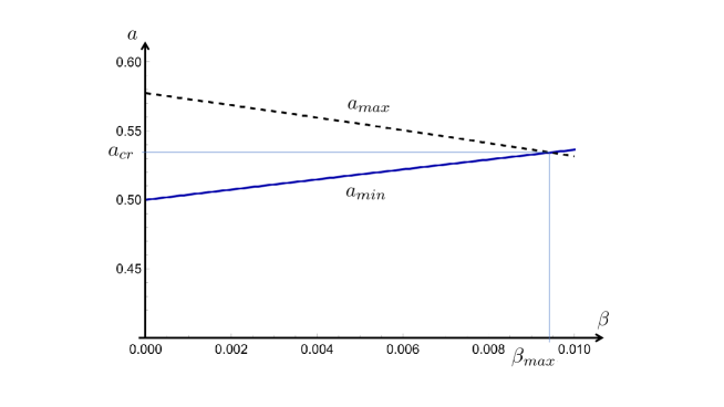
The parameter $\beta$ and $a$ are limited as $0\leq\beta\leq\beta_{max}$ and $a_{min}\leq a\leq a_{max}$ so that $mn(\theta,\phi)$ satisfies (23). In the case that $mn(\theta,\phi)$ varies maximally, namely it takes $0$ and $2\Lambda$ elsewhere, $\beta$ becomes upper bound $\beta_{max}$ , and $a_{min}$ and $a_{max}$ coincide with a value $a_{cr}$ . In Fig.1, $a_{min}$ and $a_{max}$ are shown as functions of $\beta$ , where $\beta_{max}\sim 0.009436$ and $a_{cr}\sim 0.5343$ , numerically²²2 A rough estimation of $\beta_{max}$ and $a_{cr}$ is given in Appendix. . It is interesting that even for the non-linear density contrast, $(n_{max}-n_{min})/(n_{max}+n_{min})=1$ , (54) and (53) with $\beta=\beta_{cr}$ means that the deviation of the metric functions is small in the order of $1/100$ .

Refer to caption — Figure 1: The upper bound, $a_{max}$ , and lower bound, $a_{min}$ , of $a$ are depicted as functions of $\beta$ . At $\beta=\beta_{max}$ , $a_{max}$ and $a_{min}$ coincide with $a_{cr}$ .

VI Summary

We have constructed exact static inhomogeneous solutions to Einstein’s equations with counter flow of particle fluid and a positive cosmological constant. The three-dimensional space of the solution is homothetic to a Sasakian space that consists of $S^{1}$ fibers on a $S^{2}$ base space. The solutions admit two unit Killing vector fields: timelike Killing vector field of the static spacetime, and spacelike Killing vector field that is tangent to the fiber. The unit Killing vector tangent to the fiber, whici is metric dual to the contact form of the three-dimensional space, is geodesic tangent and has non-vanishing rotation. Particles of the fluid move along geodesics whose tangent vectors are linear combinations of the two Killing vectors metioned above. Then, the geodesic congruences of the particles have non-vanishing vorticity.

On these assumptions, we have obtained reduced Einstein’s equations on the two-dimensional base space that makes a relation of the scalar curvature with the mass density of the particles, and the cosmological constant. The equation has a form of linear differential equation for the metric function. We have found exact solutions to the differential equation, where the number density of particles has non-linear inhomogeneity denoted by an arbitrary function on the base space. The solutions are inhomogeneous generalizations of Einstein’s static universe. We have presented examples of exact solutions explicitely, and we observed that the deviation of the metric is small in the order of $1/100$ for non-linear density contrast of the particles.

As is well known that Einstein’s static universe is dynamically unstable. Similarly, the solutions obtained in this paper would be unstable. It is interesting problem to extend the solutions to expanding ones with inhomogeneity.

Acknowledgements

We would like to thank K.-i. Nakao, H. Yoshino, H. Itoyama, and J. Inoguchi for valuable discussion.

Appendix A Rough estimation of $\beta_{max}$ and $a_{cr}$ of the model in Section V.3

The upper and lower limits of $a$ are determined by $mn=0$ and $mn=2\Lambda$ , respectively. Then we have

	$\displaystyle a_{max}^{2}=\frac{1}{3\Lambda}w(\theta_{-},\phi_{-};\beta),$		(57)
	$\displaystyle a_{min}^{2}=\frac{1}{4\Lambda}w(\theta_{+},\phi_{+};\beta),$		(58)

where

\displaystyle w(\theta,\phi;\beta):=1-~{}\frac{15\beta\sin 4\theta\cos\phi}{1+5\beta\sin^{3}\theta\cos\theta\cos\phi},

(59)

and $(\theta_{+},\phi_{+})$ and $(\theta_{-},\phi_{-})$ give the maximum and mminimum of $w(\theta,\phi;\beta)$ , respectively. We see that

\displaystyle\partial_{\phi}w(\theta,\phi;\beta)=0\quad\mbox{for }\phi=0,~{}\pi,

(60)

and $w(\theta,\phi;\beta)$ is invariant under

\displaystyle\phi\to\phi+\pi,\quad\theta\to\pi-\theta,

(61)

then we fix $\phi=0$ . The parameter $\beta$ should be small for positive $w(\theta,\phi;\beta)$ , then the minimum of $w(\theta,\phi;\beta)$ is attained for

\displaystyle\sin 4\theta\sim 1,\quad\sin^{3}\theta\cos\theta<0,

(62)

and maximum for

\displaystyle\sin 4\theta\sim-1,\quad\sin^{3}\theta\cos\theta<0.

(63)

Then, we have approximately

\displaystyle(\theta_{+},\phi_{+})\sim\left(\frac{7}{8}\pi,0\right)\quad\mbox{and}\quad(\theta_{-},\phi_{-})\sim\left(\frac{5}{8}\pi,0\right).

(64)

We expand (58) by the small parameter $\beta$ upto the second order as

	$\displaystyle a_{max}^{2}\sim\frac{1}{3\Lambda}(1-15\beta\sin(4\theta_{-})+75\beta^{2}\sin(4\theta_{-})\sin^{3}\theta_{-}\cos\theta_{-}),$		(65)
	$\displaystyle a_{min}^{2}\sim\frac{1}{4\Lambda}(1-15\beta\sin(4\theta_{+})+75\beta^{2}\sin(4\theta_{+})\sin^{3}\theta_{+}\cos\theta_{+}).$		(66)

For small $\beta$ , $a_{max}$ and $a_{min}$ are almost linear functions of $\beta$ as is seen in Fig. 1. By equating $a_{max}^{2}$ to $a_{min}^{2}$ , and using (64), we can estimate $\beta_{max}\sim 0.00944$ , and $a_{cr}=a_{min}=a_{max}\sim 0.534$ .

References

(1) G. Lemaître, Ann. Soc. Sci. A 53 51 (1933 ).
R. C. Tolman, Proc. Nat. Acad. Sci. 20 169 (1934).
H. Bondi, Mon. Not. R. Astron. Soc. 107 410 (1947).
(2) P. Szekeres, Commun Math Phys 41 55 (1975).
P. Szekeres, Phys Rev D 12 2941 (1975).
(3) Sasaki, Shigeo, Tohoku Math. J., Second Series 12.3 (1960) 459.
(4) D. E. Blair, ”Riemannian geometry of contact and symplectic manifolds.” Springer Science & Business Media, 2010.
(5) Manzano, Jose M., Pacific J. of Math. 270.2 (2014) 367.

Inhomogeneous Generalization of Einstein’s Static Universe with Sasakian Space