Informational Puts
Abstract
We fully characterize how dynamic information should be provided to uniquely implement the largest equilibrium in dynamic binary-action supermodular games. The designer offers an informational put: she stays silent in good times, but injects asymmetric and inconclusive public information if players lose faith. There is (i) no multiplicity gap: the largest (partially) implementable equilibrium can be implemented uniquely; and (ii) no intertemporal commitment gap: the policy is sequentially optimal. Our results have sharp implications for the design of policy in coordination environments.
1 Introduction
Many economic environments feature (i) uncertainty about a payoff-relevant fundamental state, (ii) coordination motives, and (iii) stochastic opportunities to revise actions. These elements are present across all aspects of social and economic life e.g., macroeconomics, finance, industrial organization, and political economy.111In macroeconomics, firms are uncertain about economic conditions, face complementarities (Nakamura and Steinsson, 2010), and change their prices at ticks of a Poisson clock (Calvo, 1983). In finance, creditors are uncertain about the debtor’s profitability/solvency (Goldstein and Pauzner, 2005), have incentive to run if others’ run (Diamond and Dybvig, 1983), but might only be able to withdraw their debt at staggered intervals (He and Xiong, 2012). In industrial organization, consumers are uncertain about a product’s quality, have incentive to adopt the same product as others (Farrell and Saloner, 1985; Ellison and Fudenberg, 2000), and face stochastic adoption opportunities (Biglaiser, Crémer, and Veiga, 2022).
Equilibria of such games are sensitive to dynamic information. Consider a player who, at any history of the game, finds herself with the opportunity to re-optimize her action. The fundamental state matters for her flow payoffs, so her decision must depend on her current beliefs. Moreover, since she plays the same action until she can next re-optimize, her decision also depends on her beliefs about what future agents will do. But those beliefs depend, in turn, on what she expects future players to learn, as well as their beliefs about the play of agents yet further out into the future. Thus, the stochastic evolution of future beliefs—even those arbitrarily distant—shape incentives in the present.
We are interested in dynamic information policies which fully implement the largest time path of aggregate play i.e., as a unique subgame equilibrium of the induced stochastic game. Our main result (Theorem 1) fully characterizes the form, value, and sequential optimality of designer-optimal policies:
-
1.
Form. The form of optimal dynamic information relies on the delivery of carefully chosen off-path information. If players take the designer’s preferred action, the designer stays silent. If, however, agents deviate from a target path of play specified by the policy, the designer injects an asymmetric and inconclusive public signal—this is the informational put.222This is analogous to the “Fed put” in which the Fed’s history of intervening to halt market downturns has arguably created the belief that they are insured against downside risk (Miller et al., 2002). This is as if the Fed has offered the market a put option as insurance against downturns. In our setting, the designer steps in to inject information when players start switching to action which, as we will show, with high probability induces aggregate play to correct. This is as if the designer has offered players a put option as insurance against strategic uncertainty about the play of future players.
The signal is asymmetric such that the probability that agents become a little more confident is far higher than the probability that agents become much more pessimistic. These small but high-probability movements in the direction of the dominance region—at which playing the designer’s preferred action is strictly dominant—are chained together such that the unique equilibrium of the subgame is for future players to play the designer-preferred action.333This is done via a ”contagion argument” which can be viewed as the dynamic analog of the interim deletion of strictly dominated strategies in static games of incomplete information. The signal is inconclusive such that, even if agents turn pessimistic, they do not become excessively so—this will be important for sequential optimality.
-
2.
Value. The sequentially optimal policy uniquely implements the upper-bound on the time path of aggregate play. Thus, there is no multiplicity gap: whatever can be implemented partially (i.e., as an equilibrium) can also be implemented fully (i.e., as the unique equilibrium). This is in sharp contrast to recent work on static implementation via information design in supermodular games which finds there generically exists a gap even with private information and the ability to manipulate higher-order beliefs (Morris, Oyama, and Takahashi, 2024), or with both private information and transfers (Halac, Lipnowski, and Rappoport, 2021).
-
3.
Sequential optimality. Our dynamic information policy is constructed such that at every history, the designer has no incentive to deviate.444With the caveat that for a small set of histories, deviation incentives can be made arbitrarily small. For histories where this is so, this is simply because optimal information policies continuing from those histories do not exist. Nonetheless, this can be approached via a sequence of policies so that the gap vanishes along this sequence. This openness property is also typical of static full implementation environments as highlighted by Morris, Oyama, and Takahashi (2024). Thus, there is no intertemporal commitment gap: whatever can be implemented with ex-ante commitment to the dynamic information structure can also be implemented when the sender can continually re-optimize her dynamic information.555We further emphasize that sequential optimality is not given—we offer examples of policies which are optimal but not sequentially optimal. Sequentially optimality arises through the delicate interaction between properties of our policy: asymmetry, chaining, and inconclusiveness. Asymmetric off-path information are chained together to obtain full implementation at all states in which the designer-preferred action is not strictly dominated. Then, inconclusive off-path information ensures that, even if agents turn pessimistic, full implementation is still guaranteed.
Conceptually, our contribution highlights how off-path information should be optimally deployed to shape on-path incentives. Of course, it is well-known from implementation theory (Moore and Repullo, 1988; Abreu and Matsushima, 1992) that off-path threats are powerful, albeit not sequentially optimal—if the deviation actually occurs, there is no incentive to follow-through with the policy.666With the caveat that in implementation theory, the designer’s objective function is typically not specified: we have in mind an environment in which the designer is a player in the game, and punishing players is costly. See also work on mechanism design with limited commitment (Laffont and Tirole, 1988; Bester and Strausz, 2001; Skreta, 2015; Liu et al., 2019; Doval and Skreta, 2022) and macroeconomics where time-inconsistency plays a crucial role (Halac and Yared, 2014). Information is different in two substantive ways. It is less powerful: beliefs are martingales, which imposes severe constraints on what payoffs can be delivered off-path. But it is also more flexible: the designer has the freedom to design any distribution of off-path beliefs. What should we make of these differences?
First, we will show that off-path information, through less powerful on its own, can be chained together to close the gap between full and partial implementation. Second, the flexibility of off-path information can be exploited to shape the continuation incentives of the designer. This ensures that the designer’s counterfactual selves at zero probability histories are willing to follow through with the promised information. Together, these insights offer a novel and unified treatment of dynamic information design in supermodular games.
Economically, our results have sharp implications for a range of phenomena where coordination and multiple equilbiria feature prominently e.g., in finance (debt runs, currency crises), macroeconomics (price setting), trade and industrial policy (big pushes), industrial organization (network goods), and political economy (revolutions). We briefly discuss this after stating our main result.
Related Literature
Our results relate most closely to recent work on full implementation in supermodular games via information design (Morris, Oyama, and Takahashi, 2024; Inostroza and Pavan, 2023; Li, Song, and Zhao, 2023). In this literature, information design induces non-degenerate higher-order beliefs, and this is important to obtain uniqueness via a ”contagion argument” over the type space. By contrast, our dynamic information is public and higher-order beliefs are degenerate but we leverage a distinct kind of ”intertemporal contagion”. A key takeaway from this literature is that there is typically a gap between the designer’s value under adversarial equilibrium selection, and under designer-favorable selection (what we call a “multiplicity gap”); by contrast, we show that for dynamic binary-action supermodular games there is no such gap.
Also related is the elegant and complementary work of Basak and Zhou (2020) and Basak and Zhou (2022). We highlight several substantive differences. First, we study different dynamic games: in Basak and Zhou (2020, 2022) players make a once-and-for-all decision on whether to play the risky action, and they focus on regime change games—both features play a key role in their analysis;777Basak and Zhou (2020) study a regime change game with private information where the designer can choose the frequency at which she discloses whether or not the regime has survived. Basak and Zhou (2022) study an optimal stopping game with a regime change payoff structure in which agents chooses when to undertake an irreversible risky action. in ours, agents can continually re-optimize at the ticks of their Poisson clocks and play a general binary-action supermodular game where the designer’s payoff is any increasing functional from the path of aggregate play. Importantly, our optimal dynamic information policies—and the reasons they work—are entirely distinct; we discuss this more thoroughly after stating our main result.
Our paper also relates to work on the equilibria of dynamic coordination games. An important paper of Gale (1995) studies a complete information investment game where players can decide when, if ever, to make an irreversible investment and investing is payoff dominant.888See also Chamley (1999); Dasgupta (2007); Angeletos, Hellwig, and Pavan (2007); Mathevet and Steiner (2013); Koh, Li, and Uzui (2024a) all of which study the equilibria of different dynamic coordination games. The main result is that investment succeeds across all subgame perfect equilibria. Our environment and results differ in several substantive ways. For instance, our policy allows the designer to implement the largest equilibria—irrespective of whether it is payoff dominant.999Moreover, actions in our environment are reversible, so sans any information (and assuming beliefs are not in the dominance regions) there will exist subgame perfect equilbiria in which players “cycle” between actions; this is ruled out in the environment of Gale (1995) because of irreversibility. More subtly, our dynamic information works with—but does not rely on—atomless players i.e., we obtain full implementation even if each player believes that they will not change the aggregate state. By contrast, atomic players is an essential feature of Gale (1995).
Our results are also connected to the literature on dynamic implementation. Moore and Repullo (1988) show that arbitrary social choice functions can be achieved with large off-path transfers.101010See also Aghion, Fudenberg, Holden, Kunimoto, and Tercieux (2012) for a discussion of the lack of robustness to small amounts of imperfect information, and Penta (2015) who takes a belief-free approach to dynamic implementation. Glazer and Perry (1996) show that virtual implementation of social choice functions can be achieved by appealing to extensive-form versions of Abreu and Matsushima (1992) mechanisms.111111See work by Chen and Sun (2015) who exploit the freedom to design the extensive-form. Sato (2023) designs both the extensive-form and information structure a la Doval and Ely (2020) and further utilizes the fact the designer can design information about players’ past moves; by contrast, we fix the dynamic game and past play is observed. Chen et al. (2023) weaken backward induction to initial rationalizability.121212That is, only imposing sequential rationality and common knowledge of sequential rationality at the beginning of the game, but ”anything goes” off-path; see Ben-Porath (1997). Different from these papers, our designer is substantially more constrained: (i) there is no freedom to design the extensive-form game which we take as given; (ii) the designer only offers dynamic information; and (iii) our policy is sequentially optimal.
Our game is one where players have stochastic switching opportunities. Variants of these models have been studied in macroeconomics (Diamond, 1982; Calvo, 1983; Diamond and Fudenberg, 1989; Frankel and Pauzner, 2000), industrial policy (Murphy, Shleifer, and Vishny, 1989; Matsuyama, 1991), finance (He and Xiong, 2012), industrial organization (Biglaiser, Crémer, and Veiga, 2022), and game theory (Burdzy, Frankel, and Pauzner, 2001; Matsui and Matsuyama, 1995; Oyama, 2002; Kamada and Kandori, 2020).131313See also more recent work by Guimaraes and Machado (2018); Guimaraes, Machado, and Pereira (2020). Angeletos and Lian (2016) offer an excellent survey. A common insight from this literature is that switching frictions can generate uniqueness, and the risk-dominant profile is selected via a process of backward induction. Our contribution is to show how the largest equilibrium can be uniquely implemented by carefully choosing the dynamic information policy.
Sequential optimality is an important property of our information policy and thus our work relates to recent work studying the role of (intertemporal) commitment in dynamic information design. Koh and Sanguanmoo (2022); Koh, Sanguanmoo, and Zhong (2024b) show by construction that sequential optimality is generally achievable in single-agent stopping problems. It will turn out that sequential optimal policies also exist in our environment, but for quite distinct reasons; we discuss this more thoroughly in Section 3.
2 Model
Environment
There is a finite set of states . We use to denote the set of probability measures and endow it with the Euclidian metric. There is an interior common prior and a unit measure of players indexed . Time is continuous and indexed . The action space is binary: where is ’s action at time . Write to denote the proportion of players playing action at time . Working with a continuum of agents makes our analysis cleaner because randomness from individual switching frictions vanish in the aggregate.141414By an appropriate continuum law of large numbers (Sun, 2006) where we endow the player space with the appropriate Lebesgue extension. Working with a continuum also clarifies that atomic players are not required for the use of off-path information; we discuss this in Section 4. An analog of our result holds for a finite players; we develop this in Online Appendix I.
Payoffs
The flow payoff for each player is . We write to denote the payoff difference from action relative to and assume throughout:
-
(i)
Supermodularity. is continuously differentiable and strictly increasing in .
-
(ii)
Dominant state. There exists such that .
Condition (i) states that the game is one of strategic complements. Condition (ii) is a standard richness assumption on the space of possible payoff structures: there exists some state under which playing action is strictly dominant.151515This assumption is identical to that in Morris, Oyama, and Takahashi (2024).
The payoff of player is where is an arbitrary discount rate. Each player is endowed with a personal Poisson clock which ticks at an independent rate . Players can only re-optimize at the ticks of their clocks (Calvo, 1983; Matsui and Matsuyama, 1995; Frankel and Pauzner, 2000; Frankel, Morris, and Pauzner, 2003; Kamada and Kandori, 2020). Our dynamic supermodular game is quite general with the caveat that players are homogeneous.161616A similar assumption has been made in static environments by Inostroza and Pavan (2023); Li et al. (2023) and was weakened by Morris, Oyama, and Takahashi (2024) who characterize optimal private information for full implementation by focusing on potential games with a convexity requirement, which amounts to there not being “too much heterogeneity” across players. We discuss the heterogeneous case in Section 4.
Dynamic information policies
A history specifies beliefs and aggregate play up to time . Let be the set of all histories and . Write as the natural filtration generated by histories. A dynamic information policy is a -martingale. Let
be the set of all dynamic information policies, where we emphasize that the law of can depend on past play.
Strategies and Equilibria
A strategy is a map from histories to a distribution over actions so that if ’s clock ticks at time , her choice of action is given by history .171717This is well-defined since is a.s. continuous and has left-limits. Since the measure of agents who act at time is almost surely zero, our game is in effect equivalent to one in which play at time depends on history . Given , this induces a stochastic game;181818Note that information is public so all agents share the same beliefs; in Appendix B we relax this to show that private information often cannot do better. let denote the set of subgame perfect equilibria of the stochastic game. We focus on subgame perfection because there is no private information so the game continuing from each history corresponds to a proper subgame.191919Hence, subgame perfection in our setting coincides trivially with Perfect-Bayesian Equilibria (Fudenberg and Tirole, 1991); since we are varying the dynamic information structure, this also corresponds to dynamic Bayes Correlated Equilibria (Makris and Renou, 2023)—but only in the trivial sense since higher-order beliefs are degenerate.
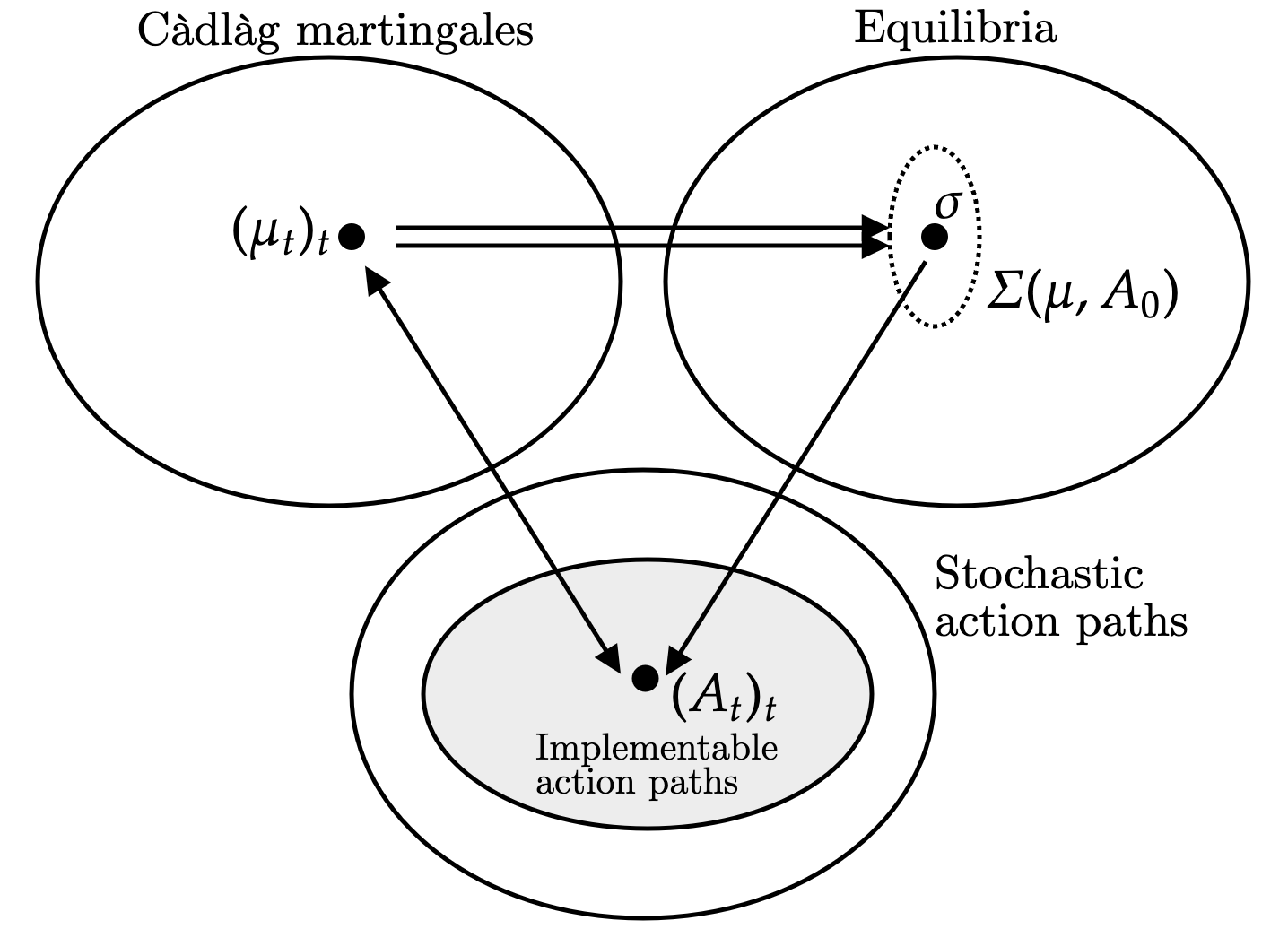
Figure 1 illustrates the connection between dynamic information policies (top left), equilibria (top right), and the path of aggregate actions (bottom). Each information policy specifies a Cadlag martingale which depends on both its past realizations, as well as past aggregate play. Given this information policy, this induces a set of equilibria . Both the realizations of beliefs as well as the selected equilibrium induce a path of aggregate play . The designer’s problem is to choose its dynamic information policy to influence the set of equilbria and thus .
Designer’s problem under adversarial equilibrium selection
The designer’s problem under commitment when nature is choosing the best equilibrium is
Conversely, when nature is choosing the worst equilibrium, the problem is
where is an increasing and bounded functional from the path-space of aggregate play e.g., the discounted measure of play with .
Sequential Optimality
If the designer cannot commit to future information, off-path delivery of information might have no bite in the present. To this end, we can define the payoff gap at history as the value of the best deviation from the original policy :
where is the filtration corresponding to . is sequentially optimal if the gap is zero for all histories . Sequential optimality is demanding and states that at every history—including off-path ones—the designer still finds it optimal to follow through with her dynamic information policy.
3 Optimal dynamic information
We begin with an intuitive description of a sequentially-optimal dynamic information policy for binary states before constructing it formally. With binary states, we set where is the dominant state. Beliefs are one-dimensional and we will directly associate . Let be the upper-dominance region: is the lowest belief such that if the current aggregate play is , playing action is strictly dominant no matter the future play of others.
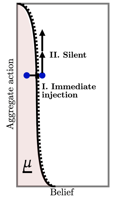
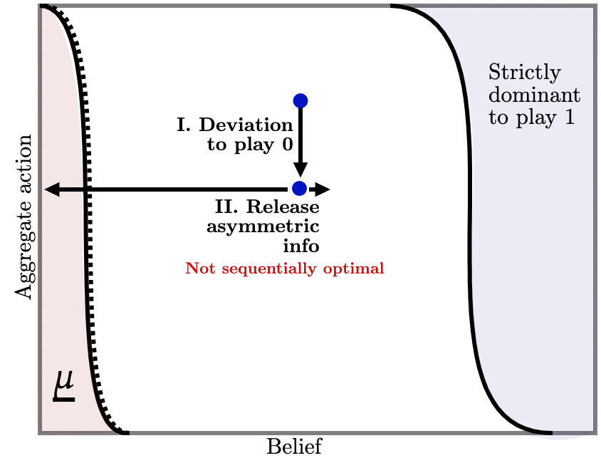
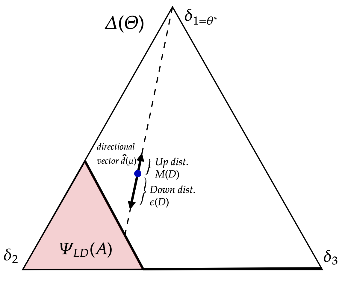
I. State is near the upper-dominance region. First suppose that at time , the public belief and aggregate play is close to the upper-dominance region as illustrated by the blue dot labelled in Figure 2b (a). If players switch to action , the designer stays silent. Thus, aggregate action progressively increases as illustrated by the upward arrows in Figure 2b (a).
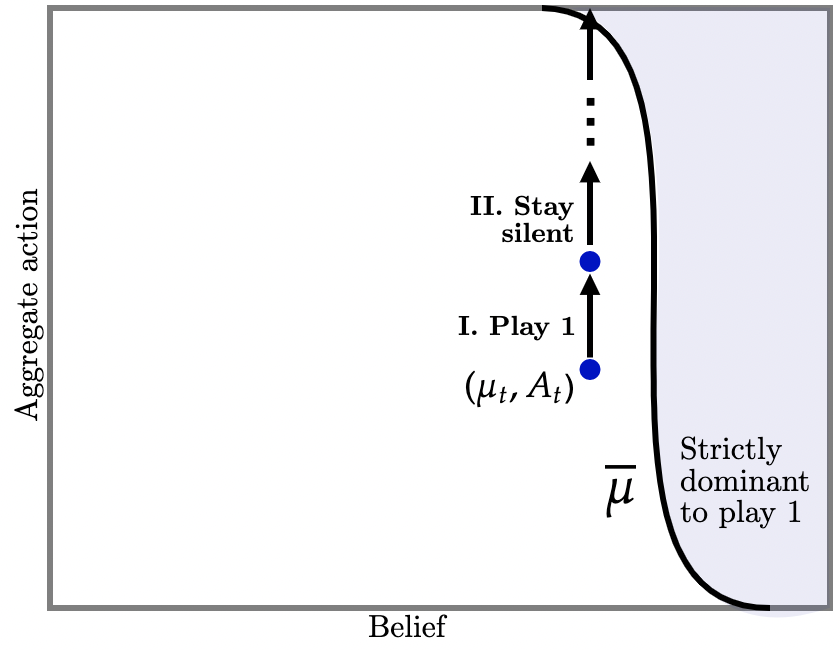
But suppose, instead, that players start playing action as depicted in Figure 2b (b) I. Then, the designer injects asymmetric information: it is very likely that agents become slightly more optimistic i.e., public beliefs move up a little and into the upper-dominance region, but there is a small chance agents become much more pessimistic (Fig. 2b (b) II). Suppose that this deviation happened and so this information is injected and, furthermore, that it has made agents a little more confident. Then, on this event, future beliefs are in the upper-dominance region so it is strictly dominant for future agents to take action . Correspondingly, the designer delivers no further information (Fig. 2b (b) III) and aggregate play begins to increase thereafter. But, knowing that this sequence of events is likely to take place, and because agents have coordination motives, deviating to action in the first place is strictly dominated.
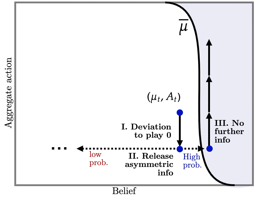
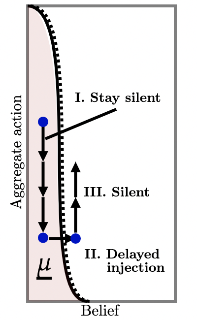
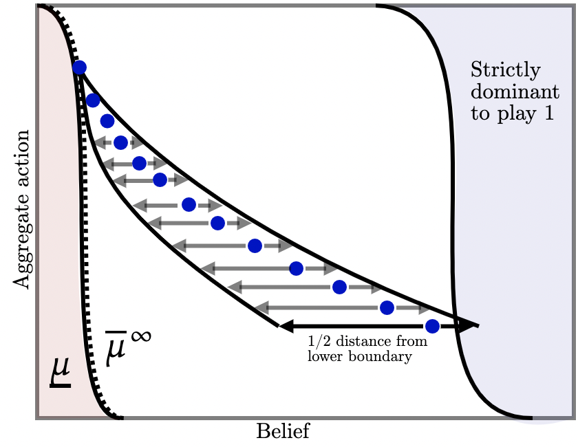
II. State is far from upper-dominance region. Next consider Figure 3b (a) where is further away from the dominance region. Our previous argument now breaks down: there is no way for off-path information—no matter how cleverly designed—to ensure beliefs reach the dominance region with a high enough probability as to deter the initial deviation to action . This is the key weakness of off-path information vis-a-vis off-path transfers. What then does the designer do?
If players start switching to , the designer delivers asymmetric information so that, with high probability, agents become a little more confident—but not confident enough that action is strictly dominant. This is depicted in Figure 3b (a) II. Upon this realization, if future agents continue deviating to , the policy injects yet another bout of asymmetric information which, with high probability, pushes beliefs into the upper-dominance region. This is depicted in Figure 3b (a) IIIB. Knowing this, we have already seen that those future agents strictly prefer to switch to . But knowing that, agents in the present state , anticipating that upon deviation the injection will, with high probability, induce future agents to play , also strictly prefer to play in the present.
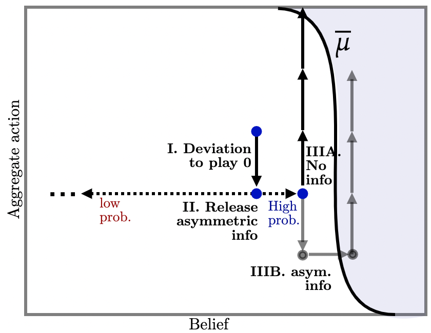
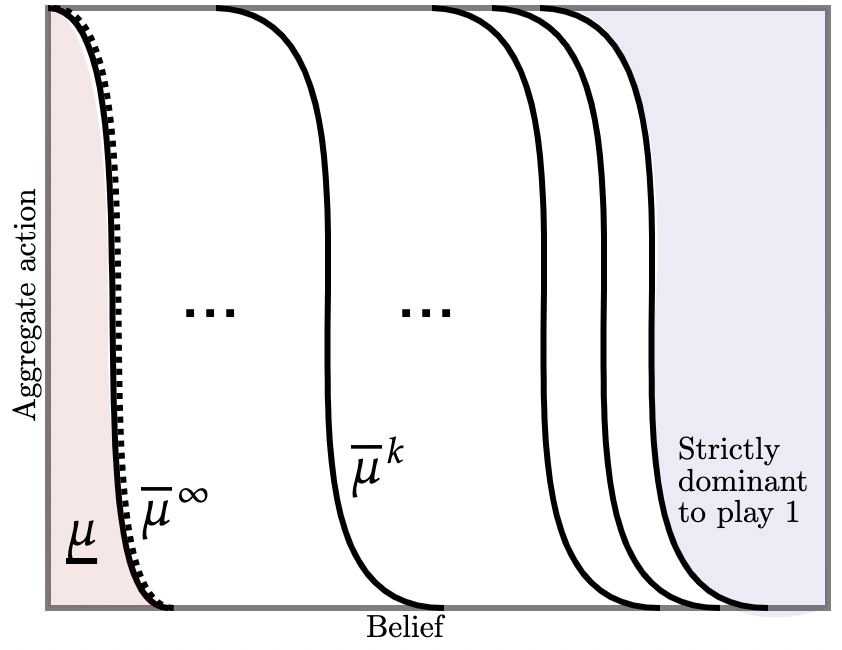
What are the limits of this line of reasoning? It turns out that by choosing our dynamic information policy carefully, we can chain together these off-path information in such a way as to obtain full implementation at all belief-aggregate pairs for which action is not strictly dominated. This is depicted by Figure (b) where, as before, the blue and pink shaded regions represent the upper- and lower-dominance regions respectively. The logic is related to the “contagion arguments” of Frankel and Pauzner (2000); Burdzy, Frankel, and Pauzner (2001); Frankel, Morris, and Pauzner (2003). These papers show that the risk-dominant action is typically selected as the limit of some iterated deletion procedure in which the blue and pink regions expand with each iteration and meet in the middle which pins down the unique equilibrium.202020In Frankel and Pauzner (2000); Burdzy, Frankel, and Pauzner (2001) this is also obtained via backward induction, where a symmetric random process governs aggregate incentives. Mapped to our model, this corresponds to public information so that the belief martingale is a time-changed Brownian motion. In Frankel, Morris, and Pauzner (2003), the this is obtained via interim deletion of strictly dominated strategies in many-action global games, though the logic is similar. By contrast, we show how dynamic information can be employed to generate asymmetric contagion such that only the upper-dominance region expands to engulf the space of all belief-aggregate play pairs where action is not strictly dominated.
III. Designer-preferred action strictly dominated. Now suppose beliefs are so pessimistic that is strictly dominated i.e., where is the highest belief under which, given , action is strictly dominated.
Then, the above policy no longer works: even if players expect all future players to switch to , they are so pessimistic about the state that switching to is strictly better. Now, the designer has to offer non-trivial information on-path to push beliefs out of the lower-dominance region. How is this optimally done?
Figure 4c (a) illustrates the optimal policy which consists of an immediate and precise injection of information such that beliefs jump to either or (just) out of the lower-dominance region. The optimality of such a policy is built on the observation that if the designer does not intervene early to curtail players from progressively switching to , it simply becomes more difficult to escape the lower-dominance region down the line. Consider, for instance, the policy in Figure 4c (b) which also injects precise information to maximize the chance of escaping the lower-dominance region, but with a delay. Before this injection, players switch to action and since is strictly decreasing, the probability of escaping the dominance region is strictly smaller. For similar reasons, the policy illustrated in Figure 4c (c) which induces continuous sample belief paths is also sub-optimal.
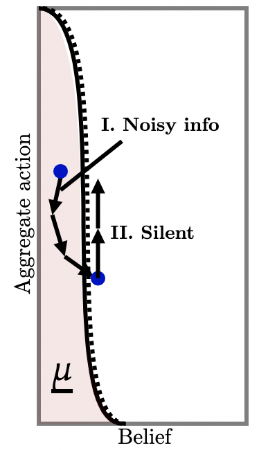
IV. Sequential optimality. Our previous discussion specified off-path injections of policies upon deviation away from the action . Of course, if such deviations actually occur, the designer may not have any incentive to follow-through with its policy. For instance, consider Figure 5b (a) which employs the strategy of injecting conclusive bad news that the state is so that, with high probability beliefs increase a little, and with low probability agents learn conclusively that . Indeed, information of this form maximizes the chance that beliefs increase212121As in Kamenica and Gentzkow (2011) and subsequent work. and, as we have described, these can be be chained together to achieve full implementation.
However, this policy is not sequentially optimal: if agents do deviate and play action , injecting such information is suboptimal because it poses an extra risk: if conclusive bad news does arrive, beliefs become absorbing at and further information is powerless to influence beliefs—it is then strictly dominant for all agents to play thereafter. How, then, is sequential optimality obtained?
Consider inconclusive off-path information as illustrated in Figure 5b (b) where each blue dot represents a potential injection of off-path information upon players’ deviating to action . Each injection induces two kinds of beliefs: upon arrival of a ‘good’ signal, agents become a little more optimistic (right arrow); upon arrival of a ‘bad’ signal, agents become relatively more pessimistic, but not so much that action becomes strictly dominated (left arrow). Figure 5b illustrates a particular policy in which, upon realization of the bad signal at state , agents’ beliefs move halfway toward the lower-dominance region i.e., to . Conversely, if the good signal arrives, believes move up a little, so that the probability of the former is much higher than the latter.
By choosing this distribution carefully for each belief-aggregate action pair, we can achieve full implementation via the chaining argument outlined above, which requires that (i) probability of the good signal arriving is sufficiently high as to deter deviations; and (ii) movement in beliefs generated by the good signal is sufficiently large that, when chained together, we obtain full implementation over the whole region. At the same time, this is sequentially optimal since, whenever the designer is faced with the prospect of injecting off-path information, she is willing to do so: with probability agents’ posterior beliefs are such that full implementation remains possible.222222We emphasize that there is nothing circular about this argument: we iteratively delete switching to action under the worst-case conjecture that, upon the bad signal arriving, all future agents play . This is sufficient to obtain full implementation as long as action is not strictly dominated.
Sequential optimality of dynamic information has been recently studied in single-agent optimal stopping problems (Koh and Sanguanmoo, 2022; Koh, Sanguanmoo, and Zhong, 2024b) who show that optimal dynamic information can always be modified to be sequentially optimal.232323See also Ball (2023) who finds in a different single-agent contracting environment that the optimal dynamic information policy happens to be sequentially optimal. In such environments, sequential optimality is obtained via an entirely distinct mechanism: the designer progressively delivers more interim information to raise the agent’s outside option at future histories which, in turn, ties the designer’s hands in the future. By contrast, in the present environment our designer chains together off-path information together to raise her own continuation value by guaranteeing that, even on realizations of the asymmetric signal, her future self can always fully implement the largest path of play.
Construction of sequentially-optimal policy.
We now make our previous discussion precise and general.
We will construct a particular martingale which is ‘Markovian’ in the sense that the ‘instantaneous’ information at time depends only on the belief-aggregate play pair , as well as an auxiliary -predictable process we will define as part of the policy. We begin with several key definitions:
Definition 1 (Lower dominance region).
Let denote the set of beliefs under which players prefer action even if all future players choose to play action :
where solves for with boundary and is independently distributed according to an exponential distribution with rate re-normalized to start at
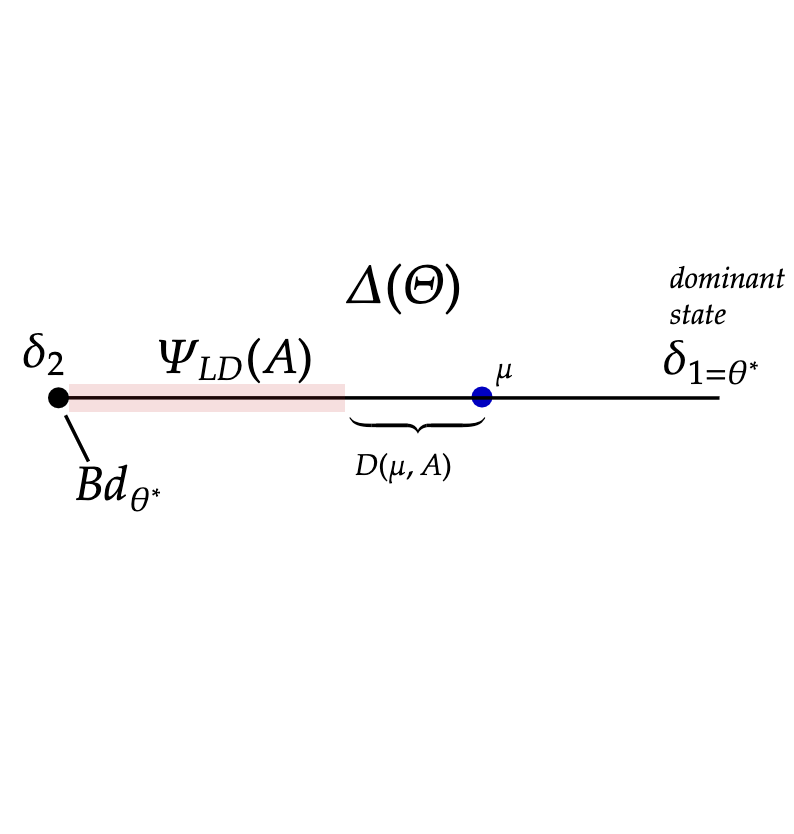
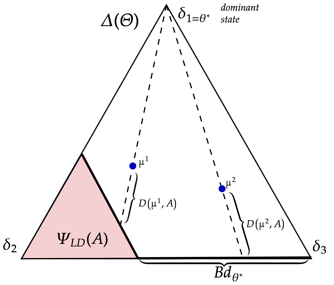
Observe that supermodularity implies is decreasing in : if . is illustrated by the pink region of Figure 6b for the cases where (panel (a)), and (panel (b)).
Definition 2.
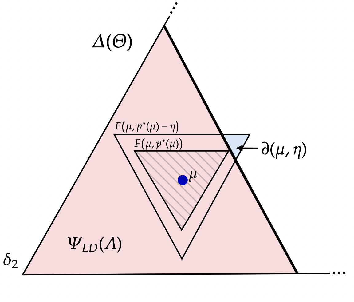
For each and , define
this gives the ‘distance’ from current beliefs as it moves along a linear path starting from to either (i) the lower dominance region ; or (ii) the set of beliefs that assign zero probability on state which we denote with This is depicted in Figure 6b where each blue dot represents a belief.
Definition 3 (Tolerance, upward/downward jump sizes, belief direction).
To describe the policy when action is not strictly dominated, we specify the following variables:
-
(i)
Tolerance. specifies the magnitude of deviation of off-path play vis-a-vis a target . If this is exceeded, the policy begins to inject additional information.
-
(ii)
Upward jump size. scales the tolerance by a factor of , and specifies the upward movement in beliefs if the injected information is positive.
-
(iii)
Downward jump size. specifies the downward movement in beliefs if the injected information is negative.
-
(iv)
Belief direction. specifies the direction of belief movements. We set it as the directional vector of towards .
Definition 3 specifies objects required to define our information policy when beliefs lie outside of the lower-dominance region . We now develop objects to define our information policy when beliefs lie inside the lower dominace region .
Definition 4 (Maximal escape probability and beliefs).
To describe the policy when action is strictly dominated, a few more definitions are in order:
-
(i)
The set of beliefs which are attainable with probability from is
which follows from the martingale property of beliefs.
-
(ii)
Maximal escape probability. is a tight upper-bound on the probability that beliefs escape .
-
(iii)
The maximal escape beliefs are
where .
We are (finally!) ready to define our dynamic information policy . Recall that is Cadlag so has left-limits which we denote with . We will simultaneously specify the law of as well as construct the stochastic process which is -predictable242424That is, is measurable with respect to the left filtration . and initializing . is interpreted as the targeted aggregate play at each history.
Given the tuple , define the time- information structure and law of motion of as follows:
-
1.
Silence on-path. If action is not strictly dominated i.e, and play is within the tolerance level i.e., then
almost surely,
i.e., no information, and
-
2.
Asymmetric and inconclusive off-path injection. If action is not strictly dominated i.e., and play is outside the tolerance level i.e., then
where is the (normalized) directional vector of toward , and reset .
-
3.
Jump. If action is strictly dominated i.e., then beliefs jump to a maximal escape point: pick any
where
We have defined a family of information structures which depend on (tolerance), (upward jump size), (downward jump size), and (distance outside the lower-dominance region ). There is some flexibility to choose them: we will set , where is a small constant, is a large constant.
We choose small so that , the upward jump size, is much smaller than the downward jump size—this ensures that the probability of becoming (a little) more optimistic is much larger. is the ratio between the upward jump size and the tolerance—it is large to guarantee that off-path information can push future beliefs into the upper-dominance region. The exact choice of and will depend on the primitives of the game, but are independent of ; a detailed construction is in Appendix A. Hence, we parameterize this family of policies by .
Theorem 1.
-
(i)
Form and value.
-
(ii)
Sequential optimality.
Proof.
See Appendix A. ∎
4 Robustness and generalizations
Our dynamic game is quite general in some regards but more specific in others. We now discuss which aspects are crucial, and which can be relaxed.
Continuum vs finite players. We worked with a continuum of players so there is no aggregate randomness in the time path of agents who can re-optimize their action.252525By a suitable continuum law of large numbers (Sun, 2006). This delivers a cleaner analysis since the only source of randomness is fluctuations in beliefs driven by policy. In Online Appendix I we show that Theorem 1 holds, mutatis mutandis, in a model with large but finite number of players.262626See Aumann (1966) and Fudenberg and Levine (1986); Levine and Pesendorfer (1995) for a discussion of the subtleties between continuum and finite players. There, we show that in a finite version of the model, the same policy that was optimal continuum case remains continues to solve problem (2) for large but finite number of players . In particular, our policy closes the multiplicity gap at rate .272727That is, ; see Online Appendix I. Mathematically, this requires more involved arguments to handle the extra randomness from switching times.
Conceptually, however, finiteness is simpler. Notice that in our continuum model, players are atomless but nonetheless off-path information is still effective. That is, players do not need to believe that they can individually influence the state for full implementation to work. This is in sharp contrast to work on dynamic coordination, durable goods monopolist, or public-good provision games which rely on the fact that each agent’s action makes a small but non-negligible difference.282828For instance Gale (1995) highlights a gap between a continuum and finite number of players in dynamic coordination games. A similar gap emerges in durable goods monopolist (Fudenberg, Levine, and Tirole, 1985; Gul, Sonnenschein, and Wilson, 1986; Bagnoli, Salant, and Swierzbinski, 1989). See also recent work by Battaglini and Palfrey (2024) in public goods context where the fact that each agent can influence the state (by a little) is important. The chief difference is that information about deviations are lost in the continuum case (Levine and Pesendorfer, 1995) which precludes the designer from detecting and responding to individual deviations.
Our key insight that this is not required: a dynamic policy with a moving target—such that asymmetric and inconclusive information is injected if aggregate play falls too far from the target—can deliver strict incentives, even if individual players cannot influence aggregate play. That is, our policy credibly insures players against paths of future play by precluding the possibility that ‘too many’ (as prescribed by the tolerance level) future agents might switch to action . In this regard working with atomless agents delivers an arguably stronger result.
Public vs private information. When the initial condition is such that playing is not strictly dominated, our policy fully implements the upper-bound on the time path of aggregate play. Thus, private information cannot do better. If initial beliefs are such that action is strictly dominated, however, this is more subtle.292929It is still an open question as to how to characterize feasible joint paths of higher-order beliefs when players also observe past play. We discuss this case in Appendix B where we construct an upper bound on the payoff difference under public and private information policies.
Homogeneous vs heterogeneous players. Payoffs in our dynamic game are quite general, with the caveat that they were identical across players. It is well-known that introducing heterogeneity typically aids equilibrium uniqueness in coordination games.303030See Morris and Shin (2006) for an articulation and survey of this idea. Thus, we expect that this can only make full implementation easier. Since we have already closed the multiplicity gap under homogeneous payoffs, qualitative features of our main result should continue to hold.313131At least when the belief-aggregate play pair is so that action is not strictly dominated.
Switching frictions. Switching frictions are commonly used to model switching costs, inattention, or settings with some staggered structure. They are important in our environment because dynamic information policy can then inject information as soon as players begin deviating from the designer’s preferred action. This allows off-path information to be chained together by correcting incipient deviations. By contrast, if players could continually re-optimize their actions, then off-path information is powerless to rule out equilibria of the form “all simultaneously switch to ”.323232Indeed, prior work which obtained equilibrium uniqueness (of risk-dominant selection) (Frankel and Pauzner, 2000; Burdzy, Frankel, and Pauzner, 2001) do so via switching frictions. Switching frictions are prevalent in macroeconomics but, as Angeletos and Lian (2016) note, “It is then somewhat surprising that this approach [combining aggregate shocks with switching frictions to generate uniqueness] has not attracted more attention in applied research.” We note, however, that it would suffice for some frictions to exist, but the exact form is not particularly important: the switching rate could vary with aggregate play, change over time, and can be taken to be arbitrarily quick or slow.
5 Discussion
We have shown that dynamic information is a powerful tool for full implementation in general binary-action supermodular games. In doing so, we highlighted key properties of off-path information: asymmetric and inconclusive signals are chained together to obtain full implementation while preserving sequential optimality. We conclude by briefly discussing implications.
Implications for implementation via information. A recent literature on information and mechanism design finds that in static environments, there is generically a multiplicity gap—the designer can do strictly better under partial rather than full implementation (Morris, Oyama, and Takahashi, 2024; Halac, Lipnowski, and Rappoport, 2021).333333See also Inostroza and Pavan (2023); Li, Song, and Zhao (2023); Morris, Oyama, and Takahashi (2022); Halac, Lipnowski, and Rappoport (2024). We show that the careful design of dynamic public information can quite generally close this gap in dynamic coordination environments.343434Moreover, information in our environment is public so higher-order beliefs are degenerate; by contrast, optimal static implementation via information typically requires inducing non-degenerate higher-order beliefs.
But do our results demand more of players’ rationality and common knowledge of rationality? Yes and no. On the one hand, it is well-known that in environments like ours, there is a tight connection between the iterated deletion of interim strictly dominated strategies (as in Frankel, Morris, and Pauzner (2003)) and backward induction, which can be viewed as the iterated deletion of intermporally strictly dominated strategies (as in Frankel and Pauzner (2000); Burdzy, Frankel, and Pauzner (2001)). In this regard, we do not think our results require ”more sophistication” of agents than in static environments. On the other hand, it is also known that common knowledge of rationality is delicate in dynamic games and must continue to hold at off-path histories.353535See Aumann (1995). Samet (2005) offers an entertaining discussion. This motivates implementation in ”initial rationalizability” when the designer has freedom to design the extensive form game (Chen, Holden, Kunimoto, Sun, and Wilkening, 2023). In this regard, our stronger results are obtained at the price of arguably stronger assumptions on common knowledge of rationality.
Implications for coordination policy. Our results have simple and sharp implications for coordination problems. It is often held that to prevent agents from playing undesirable equilbiria, policymakers must deliver substantial on-path information in order to uniquely implement the designer’s preferred action.363636See Morris and Yildiz (2019) for a recent articulation of this idea in static games, and Basak and Zhou (2020, 2022) in a dynamic regime change game where the planner uses either frequent warnings (the former), or early warnings (the latter) to implement their preferred equilibrium. Our results offer a more nuanced view.
When public beliefs are so pessimistic that the designer-preferred action is strictly dominated, an early and precise injection of on-path information is indeed required; waiting only makes implementation harder in the future. But as long as beliefs are not so pessimistic that the designer-preferred action is strictly dominated, no additional on-path information is required: silence backed by the credible promise of off-path information suffices.
References
- Abreu and Matsushima (1992) Abreu, D. and H. Matsushima (1992): “Virtual implementation in iteratively undominated strategies: complete information,” Econometrica: Journal of the Econometric Society, 993–1008.
- Aghion et al. (2012) Aghion, P., D. Fudenberg, R. Holden, T. Kunimoto, and O. Tercieux (2012): “Subgame-perfect implementation under information perturbations,” The Quarterly Journal of Economics, 127, 1843–1881.
- Angeletos et al. (2007) Angeletos, G.-M., C. Hellwig, and A. Pavan (2007): “Dynamic global games of regime change: Learning, multiplicity, and the timing of attacks,” Econometrica, 75, 711–756.
- Angeletos and Lian (2016) Angeletos, G.-M. and C. Lian (2016): “Incomplete information in macroeconomics: Accommodating frictions in coordination,” in Handbook of macroeconomics, Elsevier, vol. 2, 1065–1240.
- Arieli et al. (2021) Arieli, I., Y. Babichenko, F. Sandomirskiy, and O. Tamuz (2021): “Feasible joint posterior beliefs,” Journal of Political Economy, 129, 2546–2594.
- Aumann (1966) Aumann, R. (1966): “Existence of Competitive Equilibria in Markets with a Continuum of Traders,” Econometrica, 34, 1–17.
- Aumann (1995) Aumann, R. J. (1995): “Backward induction and common knowledge of rationality,” Games and economic Behavior, 8, 6–19.
- Bagnoli et al. (1989) Bagnoli, M., S. W. Salant, and J. E. Swierzbinski (1989): “Durable-goods monopoly with discrete demand,” Journal of Political Economy, 97, 1459–1478.
- Ball (2023) Ball, I. (2023): “Dynamic information provision: Rewarding the past and guiding the future,” Econometrica, 91, 1363–1391.
- Basak and Zhou (2020) Basak, D. and Z. Zhou (2020): “Diffusing coordination risk,” American Economic Review, 110, 271–297.
- Basak and Zhou (2022) ——— (2022): “Panics and early warnings,” PBCSF-NIFR Research Paper.
- Battaglini and Palfrey (2024) Battaglini, M. and T. R. Palfrey (2024): “Dynamic Collective Action and the Power of Large Numbers,” Tech. rep., National Bureau of Economic Research.
- Ben-Porath (1997) Ben-Porath, E. (1997): “Rationality, Nash equilibrium and backwards induction in perfect-information games,” The Review of Economic Studies, 64, 23–46.
- Bester and Strausz (2001) Bester, H. and R. Strausz (2001): “Contracting with imperfect commitment and the revelation principle: the single agent case,” Econometrica, 69, 1077–1098.
- Biglaiser et al. (2022) Biglaiser, G., J. Crémer, and A. Veiga (2022): “Should I stay or should I go? Migrating away from an incumbent platform,” The RAND Journal of Economics, 53, 453–483.
- Burdzy et al. (2001) Burdzy, K., D. M. Frankel, and A. Pauzner (2001): “Fast equilibrium selection by rational players living in a changing world,” Econometrica, 69, 163–189.
- Calvo (1983) Calvo, G. A. (1983): “Staggered prices in a utility-maximizing framework,” Journal of monetary Economics, 12, 383–398.
- Chamley (1999) Chamley, C. (1999): “Coordinating regime switches,” The Quarterly Journal of Economics, 114, 869–905.
- Chen et al. (2023) Chen, Y.-C., R. Holden, T. Kunimoto, Y. Sun, and T. Wilkening (2023): “Getting dynamic implementation to work,” Journal of Political Economy, 131, 285–387.
- Chen and Sun (2015) Chen, Y.-C. and Y. Sun (2015): “Full implementation in backward induction,” Journal of Mathematical Economics, 59, 71–76.
- Dasgupta (2007) Dasgupta, A. (2007): “Coordination and delay in global games,” Journal of Economic Theory, 134, 195–225.
- Diamond and Dybvig (1983) Diamond, D. W. and P. H. Dybvig (1983): “Bank runs, deposit insurance, and liquidity,” Journal of political economy, 91, 401–419.
- Diamond and Fudenberg (1989) Diamond, P. and D. Fudenberg (1989): “Rational expectations business cycles in search equilibrium,” Journal of political Economy, 97, 606–619.
- Diamond (1982) Diamond, P. A. (1982): “Aggregate demand management in search equilibrium,” Journal of political Economy, 90, 881–894.
- Doval and Ely (2020) Doval, L. and J. C. Ely (2020): “Sequential information design,” Econometrica, 88, 2575–2608.
- Doval and Skreta (2022) Doval, L. and V. Skreta (2022): “Mechanism design with limited commitment,” Econometrica, 90, 1463–1500.
- Ellison and Fudenberg (2000) Ellison, G. and D. Fudenberg (2000): “The neo-Luddite’s lament: Excessive upgrades in the software industry,” The RAND Journal of Economics, 253–272.
- Farrell and Saloner (1985) Farrell, J. and G. Saloner (1985): “Standardization, compatibility, and innovation,” the RAND Journal of Economics, 70–83.
- Frankel and Pauzner (2000) Frankel, D. and A. Pauzner (2000): “Resolving indeterminacy in dynamic settings: the role of shocks,” The Quarterly Journal of Economics, 115, 285–304.
- Frankel et al. (2003) Frankel, D. M., S. Morris, and A. Pauzner (2003): “Equilibrium selection in global games with strategic complementarities,” Journal of Economic Theory, 108, 1–44.
- Fudenberg and Levine (1986) Fudenberg, D. and D. Levine (1986): “Limit games and limit equilibria,” Journal of economic Theory, 38, 261–279.
- Fudenberg et al. (1985) Fudenberg, D., D. Levine, and J. Tirole (1985): “Infinite-horizon models of bargaining with one-sided incomplete information,” Game-theoretic models of bargaining, 73–98.
- Fudenberg and Tirole (1991) Fudenberg, D. and J. Tirole (1991): “Perfect Bayesian equilibrium and sequential equilibrium,” journal of Economic Theory, 53, 236–260.
- Gale (1995) Gale, D. (1995): “Dynamic coordination games,” Economic theory, 5, 1–18.
- Glazer and Perry (1996) Glazer, J. and M. Perry (1996): “Virtual implementation in backwards induction,” Games and Economic Behavior, 15, 27–32.
- Goldstein and Pauzner (2005) Goldstein, I. and A. Pauzner (2005): “Demand–deposit contracts and the probability of bank runs,” the Journal of Finance, 60, 1293–1327.
- Guimaraes and Machado (2018) Guimaraes, B. and C. Machado (2018): “Dynamic coordination and the optimal stimulus policies,” The Economic Journal, 128, 2785–2811.
- Guimaraes et al. (2020) Guimaraes, B., C. Machado, and A. E. Pereira (2020): “Dynamic coordination with timing frictions: Theory and applications,” Journal of Public Economic Theory, 22, 656–697.
- Gul et al. (1986) Gul, F., H. Sonnenschein, and R. Wilson (1986): “Foundations of dynamic monopoly and the Coase conjecture,” Journal of economic Theory, 39, 155–190.
- Halac et al. (2021) Halac, M., E. Lipnowski, and D. Rappoport (2021): “Rank uncertainty in organizations,” American Economic Review, 111, 757–786.
- Halac et al. (2024) ——— (2024): “Pricing for Coordination,” .
- Halac and Yared (2014) Halac, M. and P. Yared (2014): “Fiscal rules and discretion under persistent shocks,” Econometrica, 82, 1557–1614.
- He and Xiong (2012) He, Z. and W. Xiong (2012): “Dynamic debt runs,” The Review of Financial Studies, 25, 1799–1843.
- Inostroza and Pavan (2023) Inostroza, N. and A. Pavan (2023): “Adversarial coordination and public information design,” Available at SSRN 4531654.
- Kamada and Kandori (2020) Kamada, Y. and M. Kandori (2020): “Revision games,” Econometrica, 88, 1599–1630.
- Kamenica and Gentzkow (2011) Kamenica, E. and M. Gentzkow (2011): “Bayesian persuasion,” American Economic Review, 101, 2590–2615.
- Koh et al. (2024a) Koh, A., R. Li, and K. Uzui (2024a): “Inertial Coordination Games,” arXiv preprint arXiv:2409.08145.
- Koh and Sanguanmoo (2022) Koh, A. and S. Sanguanmoo (2022): “Attention Capture,” arXiv preprint arXiv:2209.05570.
- Koh et al. (2024b) Koh, A., S. Sanguanmoo, and W. Zhong (2024b): “Persuasion and Optimal Stopping,” arXiv preprint arXiv:2406.12278.
- Laffont and Tirole (1988) Laffont, J.-J. and J. Tirole (1988): “The dynamics of incentive contracts,” Econometrica: Journal of the Econometric Society, 1153–1175.
- Levine and Pesendorfer (1995) Levine, D. K. and W. Pesendorfer (1995): “When are agents negligible?” The American Economic Review, 1160–1170.
- Li et al. (2023) Li, F., Y. Song, and M. Zhao (2023): “Global manipulation by local obfuscation,” Journal of Economic Theory, 207, 105575.
- Liu et al. (2019) Liu, Q., K. Mierendorff, X. Shi, and W. Zhong (2019): “Auctions with limited commitment,” American Economic Review, 109, 876–910.
- Makris and Renou (2023) Makris, M. and L. Renou (2023): “Information design in multistage games,” Theoretical Economics, 18, 1475–1509.
- Mathevet and Steiner (2013) Mathevet, L. and J. Steiner (2013): “Tractable dynamic global games and applications,” Journal of Economic Theory, 148, 2583–2619.
- Matsui and Matsuyama (1995) Matsui, A. and K. Matsuyama (1995): “An approach to equilibrium selection,” Journal of Economic Theory, 65, 415–434.
- Matsuyama (1991) Matsuyama, K. (1991): “Increasing returns, industrialization, and indeterminacy of equilibrium,” The Quarterly Journal of Economics, 106, 617–650.
- Miller et al. (2002) Miller, M., P. Weller, and L. Zhang (2002): “Moral Hazard and The US Stock Market: Analysing the ‘Greenspan Put’,” The Economic Journal, 112, C171–C186.
- Moore and Repullo (1988) Moore, J. and R. Repullo (1988): “Subgame perfect implementation,” Econometrica: Journal of the Econometric Society, 1191–1220.
- Morris (2020) Morris, S. (2020): “No trade and feasible joint posterior beliefs,” .
- Morris et al. (2022) Morris, S., D. Oyama, and S. Takahashi (2022): “On the joint design of information and transfers,” Available at SSRN 4156831.
- Morris et al. (2024) ——— (2024): “Implementation via Information Design in Binary-Action Supermodular Games,” Econometrica, 92, 775–813.
- Morris and Shin (2006) Morris, S. and H. S. Shin (2006): “Heterogeneity and uniqueness in interaction games,” The Economy as an Evolving Complex System, 3, 207–42.
- Morris and Yildiz (2019) Morris, S. and M. Yildiz (2019): “Crises: Equilibrium shifts and large shocks,” American Economic Review, 109, 2823–2854.
- Murphy et al. (1989) Murphy, K. M., A. Shleifer, and R. W. Vishny (1989): “Industrialization and the big push,” Journal of political economy, 97, 1003–1026.
- Nakamura and Steinsson (2010) Nakamura, E. and J. Steinsson (2010): “Monetary non-neutrality in a multisector menu cost model,” The Quarterly journal of economics, 125, 961–1013.
- Oyama (2002) Oyama, D. (2002): “p-Dominance and equilibrium selection under perfect foresight dynamics,” Journal of Economic Theory, 107, 288–310.
- Penta (2015) Penta, A. (2015): “Robust dynamic implementation,” Journal of Economic Theory, 160, 280–316.
- Samet (2005) Samet, D. (2005): “Counterfactuals in wonderland,” Games and Economic Behavior, 51, 2005.
- Sato (2023) Sato, H. (2023): “Robust implementation in sequential information design under supermodular payoffs and objective,” Review of Economic Design, 27, 269–285.
- Skreta (2015) Skreta, V. (2015): “Optimal auction design under non-commitment,” Journal of Economic Theory, 159, 854–890.
- Sun (2006) Sun, Y. (2006): “The exact law of large numbers via Fubini extension and characterization of insurable risks,” Journal of Economic Theory, 126, 31–69.
Appendix to Informational Puts
Appendix A proves Theorem 1. Appendix B analyzes the case in which the designer can use private information.
Appendix A Proofs
Preliminaries. We use the following notation for the time-path of aggregate actions following from : for , solves
Similarly, for , solves
In words, and denote future paths of aggregate actions when everyone in the future switches to actions and as quickly as possible, respectively.
Finally, it will be helpful to define the operator mapping histories to the most recent pair of belief and aggregate action, i.e., .
Outline of proof. The proof of Theorem 1 consists of the following steps:
Step 1: We first show the result for binary states with . With slight abuse of notation, we associate beliefs directly with the probability that the state is : . Then, our lower-dominance region is one-dimensional and summarized by a threshold belief for each :
We show that implies switching to is the unique subgame perfect equilibrium under the information policy . We show this in several sub-steps.
-
•
Step 1A: There exists a belief threshold, which is a ‘rightward’ translation of the lower-dominance region such that agents find it strictly dominant to play action regardless of others’ actions if the current belief is above this threshold (Lemma 2). We call this threshold .
-
•
Step 1B: For , suppose that agents conjecture that all agents will switch to action at all future histories such that fulfills . Under this assumption, we can compute a lower bound (LB) on the expected payoff difference for agents between playing actions and for any given current belief .
To do so, we will separately consider the future periods before and after the aggregate action deviates from the tolerated distance from the target, at which point new information is provided. Call this time .
-
–
Before , we construct the lower bound using the fact that aggregate actions cannot be too far from the target even in the worst-case scenario.
-
–
At , the designer injects information with binary support. We choose the upward jump size to be sufficiently large so that, whenever the ‘good signal’ realizes beliefs exceed . Whenever the ‘bad signal’ realizes, we conjecture the worst-case that all agents switch to action .
-
–
-
•
Step 1C: We show that by carefully choosing the information policy, the threshold under which switching to is strictly dominant, , is strictly smaller than . The policy has several key features:
-
–
Large : when the aggregate action falls below the tolerated distance from the target, the high belief after the injection exceeds , which ensures the argument in Step 1B. In particular, we choose to be large relative to the Lipschitz constant of .
-
–
Small : we should maintain a low tolerance level for deviations from the target. If the designer allowed a large deviation, the aggregate action could drop so low by the time information is injected that agents’ incentives to play action would be too weak to recover.
-
–
Large : the downward jump size should be large relative to the upward jump size , but not so large that beliefs fall into the lower-dominance region. This ensures that the probability of the belief being high after the injection is sufficiently large.
These three features guarantee that the lower bound (LB) is sufficiently large and remains positive even when the current belief is slightly below . Hence is strictly smaller than , allowing us to expand the range of beliefs under which action is uniquely optimal (Lemma 3).
-
–
-
•
Step 1D: By iterating Step 1C for , we show that converges to . Then, if , agents who can switch in period find it uniquely optimal to choose action .
Step 2: We extend the arguments in Step 1 from binary states to finite states: if then playing action is the unique subgame perfect equilibrium under the information policy .
As described in the main text, our policy is such that beliefs move either in the direction toward , or in the direction away from . The key observation is that we can apply a modification of Step 1 to each direction.
Step 3: We establish sequential optimality:
-
•
Step 3A: for any , is -sequentially optimal when
-
•
Step 3B: is sequentially optimal when
Proof of Theorem 1.
Step 1. Suppose that and . With slight abuse of notation, we associate beliefs with the probability that . As in the main text, we let denote the boundary of the lower-dominance region. We will show that as long as action is not strictly dominated i.e., , then action is played under any subgame perfect equilibrium.
Definition 5.
For , we will construct a sequence where is a subset of the round- dominance region. will satisfy the following conditions:
-
(i)
Contagion. Action is strictly preferred under every history where under the conjecture that action is played under every history such that .
-
(ii)
Translation. There exists a constant such that where .
We initialize as the upper-dominance region whereby is strictly dominant.
Observe also that since is continuous and strictly increasing on a compact domain, it is also Lipschitz and we let the constant be . This also implies the lower-dominance region (as a function of ) is Lipschitz continuous, and we denote the constant with .
Lemma 1.
is Lipschitz continuous.
Proof of Lemma 1.
Fix any . The expected payoff difference between playing and when everyone in the future switches to action is given by
Note that is continuously differentiable and strictly increasing in both and . Since the domain of is compact, the following values are well-defined:
Then, for any and , we have
because the mean value theorem implies
Substituting and into the above inequality yields
where the equality follows from the definition of , i.e., for every . Hence, we have
∎
Step 1A. Construct .
Define as
with , where is defined as
is the minimum belief under which players prefer action even if all future players choose to play action .
Lemma 2.
Action is strictly preferred under every history where .
Proof of Lemma 2.
Fix any history such that Then, by the definition of , the current satisfies
Hence, action is strictly preferred regardless of others’ future play. ∎
Step 1B. Construct a lower bound for the expected payoff difference given .
Suppose that everyone plays action for any histories such that is in the round- dominance region . To obtain in Step 1C, we derive the lower bound on the expected payoff difference of playing and given .
To this end, fix any history with the current target aggregate action such that but . From our construction of we must have 373737By construction, if , must hold, which implies . If , is immediate because does not jump. For any continuous path , we define the hitting time as follows:
represents the first time at which either the designer injects new information, or the pair enters the round- dominance region. We will calculate the agent’s expected payoff before time given the continuous path and find a lower bound for this payoff by using the lower bound of for .
Before time . First, we calculate the agent’s payoff before time . Given , we have and for every because no information is injected when . Define . This implies
| (1) |
where the inequality follows from being increasing, and the last equality follows from the property that is a translation of Let , which is the aggregate play at when everyone will switch to action as fast as possible. By the definition of , we must have for every because . Then we can write down the lower bound of when as follows:
where the second inequality follows from (A). By Lipschitz continuity of we must have
| (2) |
with the Lipschitz constant . Thus, the expected payoff difference of taking action and at time given a continuous path before time is:
| (From (2)) | ||||
| (3) |
where the last inequality follows from
After time . We calculate the lower bound of the expected payoff difference after time . We know that From the definition of , we consider the following two cases depending on whether holds or not.
Case 1: . This means because no information has been injected until . Then the definition of implies where is the round- dominance region. This means every agent strictly prefers to take action 1 at . This increases , inducing every agent taking action 1 after time .383838If , then holds for any Thus, for , we have
| (4) |
where the first inequality follows from
and the second inequality follows from
Hence, by the Lipschitz continuity of , if , then
| (5) |
The expected payoff difference of taking action and at time given a path after time is
| (From (5)) | |||
| (6) |
Case 2: . By the definition of , information is injected at , and thus the belief at must be
Note that, if , then everyone strictly prefers to take action at . This increases and induces every agent to take action after time because stays in for all . Hence, we can write down the lower bound of when as follows:
where the first inequality follows from the fact that everyone in the future will switch to action in the worst-case scenario if , and the second inequality follows from (A). By Lipschitz continuity of , we must have, if , then
| (7) |
and if , then
| (8) |
Define . The expected payoff difference of taking action and at time given a path after time is
| (From (7) and (8)) | |||
| (9) |
Combining before and after time . We are ready to construct a lower bound of the expected discounted payoff difference. To evaluate , it is sufficient to focus on the case in which information is injected (Case 2) since (9) is smaller than (6) because . By taking the sum of the payoffs before and after time , that is (3) and (9), the expected payoff difference of taking action 1 and 0 at given a path is lower-bounded as follows:
| (LB) |
Intuitively, the expected payoff cannot be too low compared to the case where everyone switches to action in the future because (i) aggregate actions are close to the target before new information is injected; and (ii) if the belief jumps upward upon injection, everyone will subsequently switch to action .
Step 1C. Finally, we characterize . The following lemma establishes that under is strictly increasing in the set order.
Lemma 3.
For all , (strict inclusion).
Proof of Lemma 3.
To characterize , we first show that there exist tolerance level , upward jump magnitude and downward jump size such that if , then .
Suppose . First, we evaluate the first term of (LB). We know from the definition of the lower-dominance region that
with equality when . If , we must have , which implies
| (10) |
for some . This constant exists because
since for any . If , we have , which implies
Additionally, note that if satisfies for every , then . This follows from
where the first inequality follows from , and the second inequality follows from . Thus, if , then
| (11) |
Next, we evaluate the second term of (LB). Notice that, if , then
We will show that if . Observe that when , we must have
To see this, suppose for a contradiction that , which implies . However, since the definition of implies , we have
where the inequality follows from and the fact that is increasing in . This is a contradiction.
Lemma 1 shows that is a Lipschitz function. Since is a translation of , has the same Lipschitz constant as . Hence, if , we must have
by setting . Thus, holds, implying
We set
for a fixed small number so that and for every and (e.g., ). Thus,
| (12) |
where the last inequality follows from the continuity of and what we argued in (A) that for every .
In conclusion, we found , , and such that if , then the agent must choose action . Note that is increasing in and increasing in . Thus, is increasing in and continuous in when . Therefore, for each , there exists such that
Then we define
which also implies . From the argument above, we must have an agent always choosing action whenever (Contagion in Definition 5). Moreover, we can rewrite the above equation as follows:
where the RHS is constant in by the translation property of . Thus, must be also constant in (Translation in Definition 5). This concludes that round- dominance region satisfies because . ∎
Step 1D. In the limit, the sequence covers the region where action is not strictly dominated.
Lemma 4.
Proof of Lemma 4.
Step 2. We have constructed an information policy which uniquely implements an equilibrium achieving (2) for . we now lift this to the case with finite states as set out in the main text, where recall we set as the dominant state.
In particular, we show that if then playing action is the unique subgame perfect equilibrium under the information policy . To apply Step 1, we will construct an auxiliary binary-state environment for each direction from .
To this end, we call a vector a feasible directional vector if and but if . For each feasible directional vector , define a function such that, for every
Note that if and only if because . Observe that
where is the set of all feasible directional vectors. This is true because 1) is a polygon since the expectation operator is linear; and 2) is closed. Thus, it is equivalent to show that, for every feasible directional vector if , then playing action is the unique subgame perfect equilibrium under the information policy .
Fix a feasible directional vector Define
as the set of beliefs whose direction from is . Consider an auxiliary environment with binary state Construct a bijection such that if Denote for every . Note that .
We define a flow payoff for each player under the new environment as follows:
Define . Since is a linear map, is still continuously differentiable and strictly increasing in Also, given that , we still have an action--dominance region under this new environment.
Then we can similarly define the maximum belief under which players prefer action even if all future players choose to play action
We define . Then it is easy to see that for every and
A key observation is that if and , then every future belief must stay in almost surely with respect to any strategy. We can rewrite the time- information struture corresponding to the new environment as follows:
-
1.
Silence on-path. If and
almost surely,
i.e., no information, and
-
2.
Noisy and asymmetric off-path. If and
and reset .
By applying Step 1, we conclude that if , then action is played under any subgame perfect equilibrium. The only subtlety is to verify that as in (10), there exists a constant such that
for any feasible directional vector This is clear because for every by the definition of .
Since , we have . Hence, if , then playing action is the unique subgame perfect equilibrium under the information policy , as desired.
Step 3. We now show sequential optimality. Step 3A handles the case when beliefs are such that is strictly dominated, while 3B handles the case when is not strictly dominated.
Step 3A. is -sequentially optimal when
Fix any . Define and , i.e., and are the first times at which the belief is not in and , respectively. This means, at , all agents who can switch choose action . This pins down an aggregate action for every . Therefore, for every , implying . Thus, and so for every .
Moreover, we know that for any , so we can find an upper bound of the designer’s payoff as follows:
where satisfies , and satisfies .
For every , the optional stopping theorem implies
This implies for every By the definition of and is right-continuous, under the event . Since is convex, we also have This means , but . The definition of implies for every Thus,
This implies
Under , if then everyone takes action under any equilibrium outcome from we argued earlier. Thus,
Taking limit , we obtain
Since , we obtain .
Step 3B. We finally show is sequentially optimal when We proceed casewise:
-
•
Case 1: If and . In this case, there is no information arriving, and everyone takes action 1. This will increase , and every agent always takes action from time onwards. This is the best outcome for the designer, implying sequential optimality.
-
•
Case 2: If and . In this case, the belief moves to either or . Note that because . So no matter what information arrives, every agent takes action 1. This will increase , and every agent always takes action after time . Again, this is the best outcome for the designer, implying sequential optimality.
Appendix B Designing private information
In this appendix we discuss whether the designer can do better by designing private information.
Relaxed feasibility for joint belief processes.
We consider the relaxed problem under which each agent’s belief can be ‘separately controlled’ i.e., any joint distribution over agents’ beliefs under which the marginal distribution is a martingale is feasible under the relaxed problem. There is a common prior and a private belief process , where with being agent ’s time- filtration generated by .
The belief process for agent , is R-feasible if it is an -martingale. The set of joint R-feasible belief process is
We emphasize that this is a necessary condition on beliefs, but is not sufficient (see, e.g., Arieli, Babichenko, Sandomirskiy, and Tamuz (2021); Morris (2020) for a discussion of the static case). Let the set of feasible joint belief processes be . Although it is still an open question of how to characterize this set, we know .
The problem under private information.
noting that we have moved from subgame perfection to Perfect-Bayesian Equilibria (Fudenberg and Tirole, 1991) since there is now private information among players. However, observe that and, furthermore, that BNE coincides with SPE under public information so .
Theorem 1B.
Suppose that , then
If and further supposing is a convex functional, then
Proof.
The case in which follows directly from Theorem 1 since it already attains the upper bound on the time-path of aggregate play. We prove the second part in several steps.
Step 1A. Constructing a relaxed problem.
Some care is required in constructing the relaxed problem: by moving from to , equilibria of the resultant game might not be well-defined. We will deal with this in two ways. First, we will weaken PBE to what we call non-dominance which requires that players play action whenever it is not strictly dominated. Notice that this is not an equilibrium concept and is well-defined even with hetrogeneous beliefs. Second, we will replace the inner with to obtain the relaxed problem
It is easy to see that this is indeed a relaxed problem i.e., since (i) and furthermore, for each , .
Step 1B. Solving the relaxed problem.
First observe that for each player , a necessary condition for action to not be strictly dominated is
Hence, consider the strategy in which each player plays if and otherwise. Clearly,
Let be any Cadlag martingale and let . Clearly this Cadlag martingale is improvable if it continues to deliver information after , so it is without loss to consider which are constant a.s. after . But observe that since is a martingale, the probability of exiting the region is upper-bounded with the same calculation :
We define the (random) number of agents whose beliefs eventually cross as follows:
Consider that
Now we will derive the upper bound of for each realization of Agent takes action at time only if either
-
(I)
agent ’s Poisson clock ticked before , and his belief eventually crosses , or
-
(II)
agent took action 1 initially, and his Poisson clock has not ticked yet.
The measures of agents in (I) and (II) are and , respectively. Thus,
almost surely. Define as the solution to the ODE with boundary , and as the solution to the ODE with boundary . We have
so we can rewrite the upper bound of as follows:
almost surely. Since is a convex and increasing functional, we must have
almost surely. This implies
for every Thus,
This implies
as desired. ∎
ONLINE APPENDIX TO ‘INFORMATIONAL PUTS’
ANDREW KOH SIVAKORN SANGUANMOO KEI UZUI
Appendix I Finite players
I.1 Preliminaries
Let , where is the number of agents who initially play action . For each , define as an iid exponential distribution with rate , i.e., is agent ’s random waiting time for the first switching opportunity. We define random variables and as follows:
where is the proportion of agents playing action at time when everyone switches to action as quickly as possible, while is the auxiliary proportion of agents playing action at time when of the agents initially playing action have had opportunities to switch by time .
If the number of agents is finite, the proportion of agents playing action can deviate from the tolerated distance from the target even when no one has switched to action . The following lemma provides an upper bound on the probability of such “unlucky” events.
Lemma 5.
.
Proof.
Fix such that . We rearrange as For each , define , where , , and . If , We must have Therefore,
where the last equality follows from that if then
We define the event as follows:
Under the event , for every , we have
Note that . Thus,
where the last inequality holds if is large and . This implies
Now we compute . Note that has
| mean | |||
| variance |
Let . Thus, by Chebyshev inequality, the probability of is bounded above by
for every . Thus, the probability that the information triggers is bounded above by
since , as desired. ∎
Another subtlety with a finite number of agents is that agent ’s action today affects her future decision problem, and thus she needs to account for this effect when choosing her action today. The following lemma shows that when , it is optimal for her to take action regardless of her future actions.
Lemma 6.
For every agent , suppose be a increasing sequence of Poisson clocks of agent . Suppose be a (random) action agent takes at . If , then
Proof.
For every , consider that
where the last inequality follows from . This implies
for every , as desired. ∎
I.2 Main theorem
For simplicity, we consider binary states with . Suppose that there are agents in the economy. Let denote the set of subgame perfect equilibria of the stochastic game induced by a belief martingale under the economy consisting of agents whenever can be written as for some . We define the designer’s problem under adversarial equilibrium selection with a finite number of agents as follows:
Theorem 2.
Suppose that is Lipschitz continuous for all and and there exists a constant such that for every . Then the followings hold.
-
1.
There exists a constant such that, under any subgame perfect equilibrium ( defined in Theorem 1), an agent takes action if for every history , aggregate action , and belief ,
-
2.
There exists a constant such that, for any 393939We implicitly assume and is an integer., we have
for sufficiently large (depending on ).
-
3.
Sequential optimality:
Lemma 7.
There exists such that if , holds for all .
Proof of Lemma 7.
We follow a similar method as we did in Lemma 2. Suppose that everyone plays action 1 for any histories such that is in the round- dominance region To obtain , we derive the lower bound on the expected payoff difference of playing and given .
Fix any history with the current target aggregate action such that . From our construction of , we have . For any path with an increment at most , we define a (deterministic) hitting time as follows:
Fix , and we first determine a behavior of the path given .
Before time . For any , we showed in (A) that . By the definition of , we must have for every because for every . Then we can write down the lower bound of when as follows:
| (13) |
almost surely given .
After time . Fix any . We consider the following two cases.
Case 1: . This means because no information has been injected until . Then the definition of and the right continuity of and imply This means every agent strictly prefers to take action 1 at . This increases , inducing every agent taking action 1 after time until time at which information is injected (i.e., ).
The event that no information is injected again after time is equivalent to the event that for every . Observe that
where the first inequality follows from , and is defined as for every . By the definition of , holds, which implies the second inequality. From Lemma 5, we know that
Therefore, we can write down the lower bound of when under this case as follows:
with probability at least .
Case 2: . In this case, information is injected at . Note that, if then everyone prefers to take action 1 at . This increases inducing every agent taking action 1 after time until time at which information is injected again. Thus, the probability that and no information is injected again is at least
By definition, we have
Now we claim that
To see this, suppose for a contradiction that , which implies . However, since the definition of implies we have
where the first inequality follows from the increment size of being at most by assumption. This is a contradiction.
Hence, if ,404040We use this condition when we construct . we must have
by setting , where the second inequality follows from Lipschitz continuity of . Thus, holds, implying
for absolute constant . Then we can write down the lower bound of for every under this case as follows:
with probability at least
Combining Case 1 and Case 2, we must have
| (14) |
with probability at least
Obtaining the lower bound. Our next step is to compute the lower bound when agent takes action at time and the upper bound when agent takes action at time . One difference from the case with a continuum of agents is that agent ’s action affects the entire future path of aggregate actions. Therefore, we need to account for these effects when computing the bounds. Finally, using these bounds, we show that there exists such that if , agent strictly prefers action when , given that all agents take action for all .
Suppose that agent takes action at and takes a (random) action after each tick of her Poisson clock . We call this strategy and assume that it induces .414141Again, depends on agent ’s strategy because of finiteness. Her payoff from strategy is given by
In (13), we showed that for every 424242The increment of is at most because the probability that Poisson clocks of more than one agents tick at the same time is zero. Hence we can apply the earlier arguments. After time , if no information is injected again, everyone (including agent ) takes action , implying if . In (14), we showed
with probability at least Combining before and after , we have
with probability at least By Lipschitz continuity of and we must have434343Let and be Lipschitz constants of and , respectively. Then, is Lipschitz continuous with constant .
with probability at least Thus, for every strategy under conjecture , this implies
Now define to be a strategy that agent always takes action 1. Suppose that agent takes action 0 at the beginning for Consider that, since if ,
where the first inequality follows from Lemma 6, and the second inequality follows from (LB).
Therefore, we have
Recall that
Since holds by assumption, we must have
for some constant and such that 444444By the definition of , any and works. Let . Since we have Thus,
where these inequalities are true if
In conclusion, we have shown that there exists a constant such that if , agent strictly prefers action when , given that all agents take action for all .
Characterizing . Note that is increasing and increasing in . Thus, is increasing in and continuous in . Therefore, for each , there exists such that
if
A sufficient condition for this is
Hence, taking such that
| (15) |
is sufficient. Then we define
From the argument above, we must have an agent always choosing action whenever Moreover, we can rewrite the above equation as follows:
where the RHS is constant in by the property of . Thus, must be also constant in This concludes that round- dominance region satisfies because when is satisfied. ∎
To conclude the proof of part 1 of Theorem 2, we show the following lemma.
Lemma 8.
Proof of Lemma 8.
Proof of Part 2.
Consider the following two cases:
Case 1: . Consider large enough so that Under and the environment of agents, Part 1 implies everyone takes action 1 under any equilibrium outcome until new information is injected.
Without loss of generality, we assume Let . We have
| (Lemma 5) | |||
| () | |||
for some constant . The proof of Theorem 1 implies Thus,
when is large enough, as desired.
Let . In this case, we have
where is the maximal escaping belief defined in the main text. Under and the environment of agents, if then everyone takes action until new information is injected under any equilibrium outcome by Part 1. Thus, we have
where and satisfy
with being the number of agents playing at time . Note that the second inequality follows from Lemma 5, and the third inequality follows from . Note also that we can apply the similar argument to Lemma 5 and show that
This implies
Hence, we have
With our choice of we have there exits a constant such that as desired. ∎
Proof of Part 3.
If , consider large enough such that . We consider the following two cases for :
-
•
Case 1: If and . In this case, there is no information arriving, and everyone takes action 1. This will increase , and every agent always takes action from time onwards as long as for all . Since Lemma 5 implies that such probability converges to as , the designer’s payoff converges to the best case, implying sequential optimality as .
-
•
Case 2: If and . In this case, the belief moves to either or . Note that . So no matter what information arrives, every agent takes action 1. This will increase , and every agent always takes action after time as long as for all . Again, since such probability converges to as , we have sequential optimality as .
∎