Information upper bounds in composite quantum systems

Zhaoyang Dong College of Intelligence and Computing, Tianjin University, No.135, Ya Guan Road, Tianjin 300350, China Yuexian Hou [email protected] College of Intelligence and Computing, Tianjin University, No.135, Ya Guan Road, Tianjin 300350, China Chenguang Zhang College of Intelligence and Computing, Tianjin University, No.135, Ya Guan Road, Tianjin 300350, China School of Science, Hainan University, No.58, Renmin Avenue, Haikou 570228, China Yingjie Gao College of Intelligence and Computing, Tianjin University, No.135, Ya Guan Road, Tianjin 300350, China

Abstract

Quantum information entropy is regarded as a measure of coherence between the observed system and the environment or between many-body. It is commonly described as the uncertainty and purity of a mixed state of a quantum system. Different from traditional information entropy, we introduce a new perspective, aiming to decompose the quantum state and focus on the total amount of information contained in the components that constitute the legal quantum state itself. Based on $\chi^{2}$ divergence, we define the posterior information content of quantum pure states. We analytically proved that the upper bound of the posterior information of a 2-qubit system is exactly equal to 2. At the same time, we found that when the number of qubits $n>2$ in the quantum system, the process of calculating the upper bound of the posterior information can always be summarized as a standard semi-definite programming. Combined with numerical experiments, we generalized the previous hypothesis: A composite quantum system composed of $n$ -qubits, the upper bound of the posterior information should be equal to $n$ .

^†^†preprint: APS/123-QED

I introduction

Information and measurement are at the heart of quantum mechanics. Early in the development of quantum mechanics, Niels Bohr, Werner Heisenberg, Max Born and other physicists realised that the quantum world was fundamentally different from the classical world. In the Copenhagen interpretation, quantum state is defined as “all system information available to an observer” [1]. For example, John Archibald Wheeler attributed everything to information bits (”it from bit”) [2]. In fact, the information interpretation of quantum mechanics must clarify two fundamental questions: Where is the information of the quantum system stored? And what is the quantum information about?

Quantum information is one of the most important areas of research in quantum technology. In a general sense, quantum information refers to the computation, encoding and communication of information using various coherence of quantum systems (such as quantum parallelism, quantum entanglement etc. [3]). Until now, there has been no universally accepted unified definition of quantum information entropy. Generally, information entropy reflects the uncertainty of the system. The higher the information entropy contained in the system, the less information is required to determine a state of the system. In the classical world, information entropy generally refers to Shannon entropy [4]. Although the classical information entropy, represented by the Shannon entropy, is widely accepted by people, it does not cover the calculation of the information content when physical particles are used as information carriers in the quantum scenario. Therefore, it is natural and necessary to transition the concept of information entropy from the classical realm to the quantum realm. Quantum information entropy should not only satisfy properties such as convexity and monotonicity of classical information entropy, but also basic requirements such as non-increase of information under local operations and communication operations. In addition, the transmission and measurement of quantum information will be subject to some additional constraints due to the limitations of quantum mechanisms [5]. Some researchers have expanded information entropy to address these problems [6].

R. S. Ingarden and A. Kossakowski extended the Shannon information theory in the classical scenario to the quantum scenario based on the generalized quantum mechanism of open systems, and obtained the von Neumann entropy in the quantum version [7]. On this basis, the role of quantum characteristics such as entanglement, uncertainty and non-replicability on quantum information entropy can be examined. Due to the limitation of non-cloning under quantum mechanism, quantum information entropy does not have the ability to be copied and amplified, which is very different from classical information entropy. In addition, quantum entanglement plays a core role in distinguishing quantum information from classical information. Von Neumann entropy can be regarded as a measure of entanglement between the environment and the system when the quantum system and the environment form a pure state. Nevertheless, von Neumann entropy cannot describe more complex situations such as two-body or multi-body entanglement. For multi-body entanglement, von Neumann entropy can be expanded to quantum Rényi entropy applicable to multi-body entanglement [8]. Quantum Rényi entropy is a high-order nonlinear entropy that can directly act on the entire closed system without the need to reduce the density matrix. Moreover, due to its nonlinear characteristics, quantum Rényi entropy is more sensitive and can capture subtle entanglement [9]. The above-mentioned quantum information entropy is more oriented to the quantum theory itself. To some extent, it can be regarded as a measure of the coherence between the observation system and the environment or between multiple bodies. It cannot describe information contained in the state itself. In this sense, there is no difference in the information level between pure states.

Traditional quantum information entropy is 0 when a pure state is changed into another pure state. From the perspective of information theory, a single pure state is a definite entity. Therefore, this article starts from another perspective, focusing on the decomposition of quantum states and the total information content contained in the components that constitute the quantum state under its Bloch representation. Estimating the total information content requires analysing the relationship between components and quantum states, which is similar to quantum tomography [10, 11, 12]. It is worth emphasizing that we note the relevance of some recent influential studies to this paper [13, 14, 15, 16, 17]. Scott Aaronson proposed a shadow tomography method using semi-definite programming [13], which describe the quantum system as closely as possible by performing $M$ two-outcome measurements on multiple replicas. Instead, it might be possible to learn about a given quantum state and predict its properties using only a subset of its representations. Hsin-Yuan Huang and Richard Kueng improved Scott Aaronson’s method to construct a ”classical shadow” to predict many characteristics of the system’s quantum state through very few measurements ( $O(\log M)$ ) [14]. They believe that the number of measurements is independent of the system size and saturates information-theoretic lower bounds, and have successfully used classical systems to simulate quantum systems to some extent.

The similarity between our work and Hsin-Yuan Huang’s work is that the upper bound hypothesis of posterior information gives a lower bound on the minimum number of normalized local measurements required to estimate the state of a quantum system, because of the posterior information upper bound is invariant with respect to all possible choices of local fiducial measurements. (The results of local fiducial measurements do not provide information about unrelated regions. That is, no matter which local fiducial measurement we take, the given observational data does not change the estimate of the upper bound on the posterior information of the unknown parameters.)

The difference is that we focus on grasping the structural constraints among Bloch components of quantum states (for example: Gamel’s inequality [18]), and then estimate the information content of quantum states in composite quantum systems based on these constraint relationships, and the upper bound of the information content on quantum system is obtained. This work reveals the elegant connection between classical and quantum systems in the information sense. At the same time, it provides additional theoretical explanation and support for Hsin-Yuan Huang’s work.

The rest of this paper is organized as follows. In Sec.II, we introduce some necessary knowledge of quantum mechanics reconstructed based on the information principle. In Sec.III, we analytically proved that the posterior information upper bound of a 2-qubit space is exactly equal to 2. In Sec.IV, we extended the analysis of the general $n$ -qubit system and gave the upper bound hypothesis of the posterior information of the $n$ -qubit system. The testability of our hypothesis is based on the following theoretical observations: in a quantum system composed of $n$ -qubits, the calculation process can always be formalized into a standard semi-definite programming for solution. Hence we can conducte a large number of numerical experiments to numerically verify our hypothesis. In Sec.V, we analyze the hypothesis of the upper bound of posterior information, which leads to some of our views on composite quantum systems.

II PRELIMINARIES

II.1 General representation of 2-qubit pure states

The analysis in this work mainly focuses on the information content of the Bloch component of the 2-qubit pure state. Therefore, we first quote O. Gamel’s conclusion on quantum pure states [18].

The Bloch representation of any 2-qubit pure states $\psi=(\bm{\alpha},\bm{\beta},\bm{C})$ can be represented by the following form.

\bm{\alpha}=O_{1}\bm{\alpha^{\prime}},\ \bm{\beta}=O_{2}\bm{\beta^{\prime}},\ \bm{C}=O_{1}\bm{C^{\prime}}O_{2}^{T}

(1)

where:

\bm{\alpha^{\prime}}=\begin{pmatrix}\cos\theta\\ 0\\ 0\end{pmatrix},\bm{\beta^{\prime}}=\begin{pmatrix}\cos\theta\\ 0\\ 0\end{pmatrix},\bm{C^{\prime}}=\begin{pmatrix}1&0&0\\ 0&\sin\theta&0\\ 0&0&-\sin\theta\end{pmatrix}

(2)

$O_{1}$ , $O_{2}\in SO(3)$ are respectively three-dimensional rotation matrices:

	$\displaystyle O_{1}$	$\displaystyle=\begin{pmatrix}\cos\phi cosk&\cos\omega sink+\sin\omega sin\phi cosk&\sin\omega sink-\cos\omega sin\phi cosk\\ -\cos\phi sink&\cos\omega cosk-\sin\omega sin\phi sink&\sin\omega cosk+\cos\omega sin\phi sink\\ \sin\phi&-\sin\omega cos\phi&\cos\omega cos\omega\end{pmatrix}$		(3)
	$\displaystyle O_{2}$	$\displaystyle=\begin{pmatrix}\cos\phi^{\prime}\cos k^{\prime}&\cos\omega^{\prime}\sin k^{\prime}+\sin\omega^{\prime}\sin\phi^{\prime}\cos k^{\prime}&\sin\omega^{\prime}\sin k^{\prime}-\cos\omega^{\prime}\sin\phi^{\prime}\cos k^{\prime}\\ -\cos\phi^{\prime}\sin k^{\prime}&\cos\omega^{\prime}\cos k^{\prime}-\sin\omega^{\prime}\sin\phi^{\prime}\sin k^{\prime}&\sin\omega^{\prime}\cos k^{\prime}+\cos\omega^{\prime}\sin\phi^{\prime}\sin k^{\prime}\\ \sin\phi^{\prime}&-\sin\omega^{\prime}\cos\phi^{\prime}&\cos\omega^{\prime}\cos\omega^{\prime}\end{pmatrix}$		(3)

where $\theta$ can always be in the first quadrant. In other words, $\sin\theta$ and $\cos\theta$ can always be positive numbers. Because, we can use a group of local transformations $O_{1},O_{2}$ to transform any $\theta^{\prime}$ that doesn’t in the first quadrant into $\theta$ that in the first quadrant.

It is obvious that the two three-dimensional local rotations each have three degrees of freedom, and Eq.2 contains one degree of freedom. There are 7 degrees of freedom in the general representation of the 2-qubit pure state system (Considering the unimportance of the global phase).

In the form of Bloch representation, the standard quantum state $\psi$ contains a total of 16 elements and is usually represented as a vector of $16\times 1$ .

{\psi}=\left(b_{1},b_{2},b_{3},\ldots,b_{i},\ldots,b_{16}\right)^{T}

(4)

where $b_{i}$ represents the parameter of the Bloch vector. $b_{1}=1$ is the dummy component and can usually be omitted.

II.2 Information divergence

The information impact of random events is determined by the difference in the probability distribution describing the system state before and after the event occurs. Rényi gave a general family of difference measures for probability distribution, which can take different forms depending on the different definitions of its generating function $f$ [19].

\begin{split}D_{f}(P||Q)\equiv\int_{\Omega}f\left(\frac{dP}{dQ}\right)dQ\end{split}

(5)

The analysis in this article will be mainly based on a special $f$ divergence defined by Eq.5, namely the $\chi^{2}$ divergence. It is shown to be an upper bound of the Kullback-Leibler divergence with the base natural logarithm [20], and hence is of statistical relevance, since it is well-known that Kullback-Leibler divergence is a local approximation of the rigorously established Fisher-Rao distance.

The generating function of $\chi^{2}$ divergence is defined as $f(t)\equiv(t-1)^{2}$ and it has the following form:

\begin{split}D_{\chi^{2}}(P||Q)\equiv\int_{\Omega}\left(\frac{dP}{dQ}-1\right)^{2}dQ=\int_{\Omega}\frac{dP^{2}}{dQ}-1\end{split}

(6)

When considering discrete probability distributions, $P$ and $Q$ can be corresponding to a set of probability terms $\{p_{i}\}$ or $\{q_{i}\}$ that satisfy the normalization condition, where $\sum p_{i}=1,\,\sum q_{i}=1$ .

\begin{split}D_{\chi^{2}}(P||Q)\equiv\sum\nolimits_{{}i}\left(\frac{p_{i}}{q_{i}}-1\right)^{2}\cdot q_{i}=\left(\sum\nolimits_{i}\frac{p^{2}_{i}}{q_{i}}\right)-1\end{split}

(7)

Therefore, we give the information content based on the $\chi^{2}$ distance definition.

Definition 1 ( $\chi^{2}$ distance information content).

According to the form of Bloch vector in Eq.4, the $\chi^{2}$ distance information content of a general qubit $\psi$ is defined as:

I_{\chi^{2}}(\psi)=\sum_{i}^{d}D_{X^{2}}(b_{i},h_{i})

(8)

where $D_{\chi^{2}}(b_{i},h_{i})$ is the $\chi^{2}$ distance of the $i$ -th component $b_{i}$ of the Bloch vector $\psi$ relative to the $i$ -th component $h_{i}$ of the comparison benchmark vector. According to the relationship between Bloch vector and probability, and the calculation formula of $\chi^{2}$ distance [21], then

D_{\chi^{2}}(b_{i},h_{i})=\frac{(\frac{b_{i}+1}{2})^{2}}{\frac{h_{i}+1}{2}}+\frac{(\frac{1-b_{i}}{2})^{2}}{\frac{1-h_{i}}{2}}-1

(9)

III The information upper bound of pure state in 2-qubit system

For the general 2-qubit pure state given above, it is not difficult to find through Eq.1-3 that once some components in the 16-dimensional vector are determined, the remaining components will be uniquely determined (In extreme cases , when $b_{2},\ldots,b_{15}$ are determined, $b_{16}$ can certainly be calculated directly), that is, the 16-dimensional components of the Bloch vector are not independent of each other. Components that can be determined by preceding components do not provide any additional information, so when calculating the information capacity, this part of the redundancy should be removed. Therefore, we give the posterior information definition based on Eq.8:

Definition 2 (The posterior $\chi^{2}$ divergence information content).

For the Bloch vector of the 2-qubit pure state, starting from $b_{1}$ and based on the determined components, the possible maximum value $b_{i}^{max}$ and minimum value $b_{i}^{min}$ of the current component $b_{i}$ are calculated. According the maximum entropy estimation principle, $(b_{i}^{max}+b_{i}^{min})/2$ is the comparison benchmark $h_{i}$ of $b_{i}$ .

The posterior $\chi^{2}$ divergence information content of the Bloch vector of 2-qubit system is

I_{\chi^{2},post}({\psi})=\sum_{i=2}^{16}D_{\chi^{2}}(b_{i},\frac{b_{i}^{max}+b_{i}^{min}}{2})

(10)

The analysis in this paper does not rely on the prior information, so please refer to Appendix B for the definition of the prior information content.

Remark.

The meaning of a prior information used here is: the information content obtained by calculation without any structural knowledge about the quantum state space (this structural knowledge can be considered empirical). Posterior information refers to the information content obtained by calculation with structural knowledge about the quantum state space. Therefore, the difference between a prior information and posterior information lies in whether quantum state space structure information (from experience) is used.

In addition, the $\chi^{2}$ divergence determined by the Bloch component satisfies the following Pythagorean relationship.

Lemma 1 (Pythagorean properties).

Assume that $t_{1}$ , $t_{2}$ , $t_{3}$ are components of the Bloch vector, and $t_{1}^{2}=t_{2}^{2}+t_{3}^{2}$ . then:

D_{X^{2}}(t_{1},0)\equiv D_{X^{2}}(t_{2},0)+D_{X^{2}}(t_{3},0)

(11)

Proof.

The proof is given in Appendix C. ∎

Lemma 1 allows us to calculate the information content of each Bloch component in pieces.

One reason for calculating posterior information based on pure state space structures is that the information contained in pure state space structures is pure quantum, that is, there is no uncertainty (information) caused by classical probability mixing. According to Eq.1-3, we can see that for any pure states, only the norms of $\bm{\alpha}$ and $\bm{\beta}$ are required to be equal, and no additional constraints are required between them, that is, their comparison benchmark is always 0 and the posterior information content is equal to the prior information content. Therefore only the components in matrix $\bm{C}$ need to be discussed.

As a result, we have the following lemma.

Lemma 2 (Unique determination).

For a Bloch vector of pure state in 2-qubit system $\psi=(\bm{\alpha},\bm{\beta},\bm{C})$ with $\cos^{2}\phi\cos^{2}k\neq 0$ or $\cos^{2}\phi^{\prime}\cos^{2}k^{\prime}\neq 0$ , when $\bm{\alpha}$ , $\bm{\beta}$ and the first two components $c_{11}$ , $c_{12}$ in the matrix $\bm{C}$ are determined, then the remaining components of this Bloch vector are uniquely determined.

Proof.

The proof is given in Appendix D. ∎

The above lemma 2 is for the general case. In particular, when $\cos^{2}\phi\cos^{2}k=0$ or $\cos^{2}\phi^{\prime}\cos^{2}k^{\prime}=0$ , it corresponds to several special cases. In these cases, the structure constraints of the 2-qubit system will be weakened, some components in the quantum state will be uniquely determined by $\bm{\alpha}$ and $\bm{\beta}$ , and only two additional components ({ $c_{12},c_{13}$ } or { $c_{21},c_{22}$ }) need to be determined. When calculating the information content, there are only $(\omega+\omega^{\prime})$ in the parametric equation, so their comparison benchmark is all 0. Obviously, it can be concluded that their posterior information content is less than 2. Therefore, we will not go into details of these special cases in this article.

Expand and calculate the matrix $\bm{C}$ . Obviously, the sign of the component $\cos\phi$ , $\cos{\phi^{\prime}}$ , $\cos{k}$ , $\cos{k^{\prime}}$ does not affect the determination of the components in $\bm{C}$ . In particular, the first two components $c_{11}$ and $c_{12}$ in the $\bm{C}$ matrix can be represented by components:

\displaystyle c_{11}

\displaystyle=

\displaystyle\cos\phi coskcos\phi^{\prime}cosk^{\prime}-\sin\theta\sqrt{1-\cos^{2}\phi cos^{2}k}\sqrt{1-\cos^{2}\phi^{\prime}cos^{2}k^{\prime}}\cos(\omega+\omega^{\prime}+\omega_{1}+\omega_{1}^{\prime})

(12)

\displaystyle c_{12}

\displaystyle=

\displaystyle-\cos\phi coskcos\phi^{\prime}cosk^{\prime}+\sin\theta\sqrt{1-\cos^{2}\phi cos^{2}k}\sqrt{1-\cos^{2}\phi^{\prime}cos^{2}k^{\prime}}\sin(\omega+\omega^{\prime}+\omega_{1}+\omega_{2}^{\prime})

(13)

where

		$\displaystyle\sin\omega_{1}=\frac{\sin k}{\sqrt{\sin^{2}k+\sin^{2}\phi\cos^{2}k}},\sin\omega_{1}^{{}^{\prime}}=\frac{\sin k^{{}^{\prime}}}{\sqrt{\sin^{2}k+\sin^{2}\phi^{{}^{\prime}}\cos^{2}k^{{}^{\prime}}}},\sin\omega_{2}^{{}^{\prime}}=\frac{\cos k^{{}^{\prime}}}{\sqrt{\cos^{2}k^{{}^{\prime}}+\sin^{2}\phi^{{}^{\prime}}\sin^{2}k^{{}^{\prime}}}}$		(14)
		$\displaystyle\cos\omega_{1}=\frac{\sin\phi\text{cos}k}{\sqrt{\sin^{2}k+\sin^{2}\phi\text{cos}^{2}k}},\cos\omega_{1}^{{}^{\prime}}=\frac{\sin\phi^{{}^{\prime}}\cos k^{{}^{\prime}}}{\sqrt{\sin^{2}k^{{}^{\prime}}+\sin^{2}\phi^{{}^{\prime}}\cos^{2}k^{{}^{\prime}}}},\cos\omega_{2}^{{}^{\prime}}=\frac{\sin\phi^{{}^{\prime}}\sin k^{{}^{\prime}}}{\sqrt{\cos^{2}k^{{}^{\prime}}+\sin^{2}\phi^{{}^{\prime}}\sin^{2}k^{{}^{\prime}}}}$		(14)

In order to facilitate subsequent analysis, we let $\mu=\cos\theta$ , $a_{1}=\cos\phi\cos k$ , $a_{2}=\cos\phi\sin k$ , $a_{3}=\sin\phi$ , $b_{1}=\cos\phi^{\prime}\cos k^{\prime}$ , $b_{2}=\cos\phi^{\prime}\sin k^{\prime}$ , $b_{3}=\sin\phi^{\prime}$ . The form of $\bm{\alpha}$ and $\bm{\beta}$ become as follows:

\bm{\alpha}=\left(\begin{array}[]{c}{\mu\cos\phi\cos k}\\ {-\mu\cos\phi\sin k}\\ {\mu\sin\phi}\\ \end{array}\right)=\left(\begin{array}[]{c}{\mu a_{1}}\\ {-\mu a_{2}}\\ {\mu a_{3}}\\ \end{array}\right)

(15)

\bm{\beta}=\left({\begin{array}[]{*{20}{c}}{\mu\cos\phi^{\prime}\cos k^{\prime}}\\ {-\mu\cos\phi^{\prime}\sin k^{\prime}}\\ {\mu\sin\phi^{\prime}}\end{array}}\right)=\left({\begin{array}[]{*{20}{c}}{\mu{b_{1}}}\\ {-\mu{b_{2}}}\\ {\mu{b_{3}}}\end{array}}\right)

(16)

$c_{11}$ and $c_{22}$ in Eq.12,13 can be represented as:

$\displaystyle c_{11}$	$\displaystyle=a_{1}b_{1}-\sqrt{(1-\mu^{2})(1-a_{1}^{2})(1-b_{1}^{2})}$	(17)
	$\displaystyle\qquad\times\cos(\omega+\omega^{\prime}+\omega_{1}+\omega_{1}^{\prime})$
$\displaystyle c_{12}$	$\displaystyle=-a_{1}b_{2}+\sqrt{(1-\mu^{2})(1-a_{1}^{2})(1-b_{2}^{2})}$
	$\displaystyle\qquad\times\sin(\omega+\omega^{\prime}+\omega_{1}+\omega_{2}^{\prime})$

Obviously, if we consider the parameters $\omega$ and $\omega^{\prime}$ as variables and the other parameters as constants. The upper and lower bounds of components $c_{11}$ and $c_{22}$ can be represented as:

		$\displaystyle c_{11}^{max}\begin{aligned} =a_{1}b_{1}+\sqrt{(1-\mu^{2})(1-a_{1}^{2})(1-b_{1}^{2})}\end{aligned}$		(18)
		$\displaystyle c_{11}^{min}=a_{1}b_{1}-\sqrt{(1-\mu^{2})(1-a_{1}^{2})(1-b_{1}^{2})}$
		$\displaystyle c_{12}^{max}=-a_{1}b_{2}+\sqrt{(1-\mu^{2})(1-a_{1}^{2})(1-b_{2}^{2})}$
		$\displaystyle c_{12}^{min}=-a_{1}b_{2}-\sqrt{(1-\mu^{2})(1-a_{1}^{2})(1-b_{2}^{2})}$

the comparison benchmark $c_{11}^{avg}$ and $c_{12}^{avg}$ is:

	$\displaystyle c_{11}^{avg}$	$\displaystyle=\frac{c_{11}^{max}+c_{11}^{min}}{2}=a_{1}b_{1}$		(19)
	$\displaystyle c_{12}^{avg}$	$\displaystyle=\frac{c_{12}^{max}+c_{12}^{min}}{2}=-a_{1}b_{2}$		(19)

In order to prove the upper bound of the posterior information content of the 2-qubit system, we will construct the following lemma:

Lemma 3.

For any 2-qubit pure state Bloch vectors $\psi$ with $\mu=0$ ,

I_{\chi^{2},post}(\psi)=2

(20)

Proof.

When $\mu=\mathrm{cos}\theta=0$ , $|\mathrm{sin}\theta|=1$ . At this time, the quantum state $\psi$ is in the maximum entangled state. According to Eq. 2, the correlation matrix $\bm{C}$ must be an orthogonal matrix and the modulus of each row and column is 1 (because $\bm{C}=O_{1}\bm{C}_{0}O_{2}^{\mathrm{T}}$ is obtained by multiplying three orthogonal matrices). After the first two rows of the orthogonal matrix $\bm{C}$ are determined, the third row is naturally determined, so no posterior information is provided. And since $\bm{\alpha}$ and $\bm{\beta}$ are both $\bm{0}$ and also do not provide any information, then according to Lemma 1.

I_{\chi^{2},post}(\psi)=1^{2}+|\mathrm{sin}\theta|^{2}=2

(21)

∎

Lemma 4.

For any 2-qubit pure state Bloch vectors $\psi$ with $|\mu|=1$ ,

I_{\chi^{2},post}(\psi)=2

(22)

Proof.

When $|\mu|=1$ , the quantum state is in a tensor product state. $\bm{\alpha}$ and $\bm{\beta}$ in the Bloch vector cannot constrain each other, so the information provided by $\bm{\alpha}$ and $\bm{\beta}$ is all posterior information. For given $\bm{\alpha}$ and $\bm{\beta}$ , the parameters $\phi,k,\phi^{\prime},k^{\prime}$ can be determined, and only two parameters $\omega$ and $\omega^{\prime}$ are undetermined at this time. Since $|\mu|=|\mathrm{cos}\theta|=1$ , then $\mathrm{sin}\theta=0$ . $C^{\prime}$ can be obtained

C^{\prime}=\begin{pmatrix}1&0&0\\ 0&0&0\\ 0&0&0\end{pmatrix}

(23)

By directly calculating each element in the correlation matrix $\bm{C}$ , it is not difficult to find that $\omega$ and $\omega^{\prime}$ do not affect any components in $\bm{C}$ . Therefore, the upper and lower bounds of each element in $\bm{C}$ are equal and no posterior information is provided. At this time, the information held by Bloch vector is completely provided by $\bm{\alpha}$ and $\bm{\beta}$ . Then

I_{\chi^{2},post}(\psi)=2

(24)

∎

Lemma 5.

For any 2-qubit pure state Bloch vectors $\psi$ with $|\mu|\in(0,1)$ ,

I_{\chi^{2},post}(\psi)<2

(25)

Proof.

Without loss of generality, assume $c_{11}^{avg}$ and $c_{12}^{avg}$ are both positive. $\theta$ is in the first quadrant, then $\mu=\cos\theta\in(0,1)$ . Directly calculate the posterior information content of the quantum state at this time:

	$\displaystyle I_{\chi^{2},\text{post}}(\psi)=$	$\displaystyle 2D_{\chi^{2}}(\mu,0)+D_{\chi^{2}}(c_{11}^{\text{max}},c_{11}^{avg})$		(26)
		$\displaystyle+D_{\chi^{2}}(c_{12}^{\text{max}},c_{12}^{a\nu g})$		(26)

For the convenience of proof, let $\delta=(1-\mu^{2})(1-a_{1}^{2})(1-b_{1}^{2})$ in Eq.18. According to Eq.8, calculate the posterior information content:

$\displaystyle D_{\chi^{2}}(c_{11}^{max},c_{11}^{avg})$	$\displaystyle=\frac{(\frac{a_{1}b_{1}+\sqrt{\delta}+1}{2})^{2}}{\frac{a_{1}b_{1}+1}{2}}+\frac{(\frac{1-a_{1}b_{1}-\sqrt{\delta}}{2})^{2}}{\frac{1-a_{1}b_{1}}{2}}-1\quad$	(27)
	$\displaystyle=\frac{(a_{1}b_{1}+1)^{2}+\delta+2(a_{1}b_{1}+1)\sqrt{\delta}}{2(a_{1}b_{1}+1)}+\frac{(1-a_{1}b_{1})^{2}+\delta-2(1-a_{1}b_{1})\sqrt{\delta}}{2(1-a_{1}b_{1})}-1$
	$\displaystyle=\frac{(a_{1}b_{1}+1)(1-a_{1}^{2}b_{1}^{2})+(1-a_{1}b_{1})(1-a_{1}^{2}b_{1}^{2})+2\delta}{2(1-a_{1}^{2}b_{1}^{2})}-1$
	$\displaystyle=\frac{\delta}{1-a_{1}^{2}b_{1}^{2}}$

Similarly, $D_{\chi^{2}}(c_{12}^{\text{max}},c_{12}^{avg})$ can perform similar calculations. The posterior information content in Eq.26 can be organized into the following form.

\begin{array}[]{l}{I_{{\chi^{2}},post}}(\psi)=\\ \quad 2{D_{{\chi^{2}}}}(\mu,0)+\frac{{(1-{\mu^{2}})(1-a_{1}^{2})(1-b_{1}^{2})}}{{1-a_{1}^{2}b_{1}^{2}}}+\frac{{(1-{\mu^{2}})(1-a_{1}^{2})(1-b_{2}^{2})}}{{1-a_{1}^{2}b_{2}^{2}}}\end{array}

(28)

let $x_{1}=a_{1}^{2}$ , $y_{1}=b_{1}^{2}$ , $y_{2}=b_{2}^{2}$ . Then, this problem is organized into a discussion of the following functions:

\begin{array}[]{l}f(x_{1},y_{1},y_{2})=\\ \quad 2D_{\chi^{2}}(\mu,0)+\frac{(1-\mu^{2})(1-x_{1})(1-y_{1})}{1-x_{1}y_{1}}+\frac{(1-\mu^{2})(1-x_{1})(1-y_{2})}{1-x_{1}y_{2}}\end{array}

(29)

where $x_{1},y_{1},y_{2}\in[0,1]$ , and $0\leq y_{1}+y_{2}\leq 1$ . The partial derivative of the function $f(x_{1},y_{1},y_{2})$ with respect to $x_{1}$ .

\begin{array}[]{c}\frac{\partial f(x_{1},y_{1},y_{2})}{\partial x_{1}}=\frac{-(1-\mu^{2})(1-y_{1})^{2}}{(1-x_{1}y_{1})^{2}}+\frac{-(1-\mu^{2})(1-y_{2})^{2}}{(1-x_{1}y_{2})^{2}}\end{array}

(30)

Obviously, $\frac{\partial f(x_{1},y_{1},y_{2})}{\partial x_{1}}\leq 0$ , the equation holds if and only if $y_{1}=y_{2}=1$ . Due to the constraint $0\leq y_{1}+y_{2}\leq 1$ , the equation is not satisfied within the current range of values. Therefore, $f(x_{1},y_{1},y_{2})$ is monotonically decreasing in the $x_{1}$ direction. This means that for the optimization problem of $f(x_{1},y_{1},y_{2})$ , only need to consider the optimal value of $f(0,y_{1},y_{2})$ in the extreme case of $x_{1}=0$ . That is:

f(0,y_{1},y_{2})=2D_{\chi^{2}}(\mu,0)+(1-\mu^{2})(2-y_{1}-y_{2})

(31)

Consider the two directions $y_{1}$ and $y_{2}$ :

\frac{\partial f(0,y_{1},y_{2})}{\partial y_{1}}=\frac{\partial f(0,y_{1},y_{2})}{\partial y_{2}}=-(1-\mu^{2})<0

(32)

At this time, $f(0,y_{1},y_{2})$ is monotonically decreasing in both $y_{1}$ and $y_{2}$ directions. Therefore, when $y_{1}=y_{2}=0$ , $f(0,y_{1},y_{2})$ has a maximum value, and the maximum value is:

\bm{g}(\mu)=2D_{X^{2}}(\mu,0)+2(1-\mu^{2})=2

(33)

where $\mu\in(0,1)$ . Based on the above analysis, it can be proved that in the current range, $f(x_{1},y_{1},y_{2})\leq 2$ holds. That is

I_{{\chi^{2}},post}(\psi)\leq 2

(34)

∎

Lemma 3, lemma 4 and lemma 5 cover all Bloch vectors of 2-qubit pure state system, the following theorem has been proven to be true.

Theorem 1.

The upper bound on the posterior information content of a 2-qubit pure state system is exactly equal to 2.

IV The information upper bound of pure state in n-qubit system

We next generalize Theorem 1 to n-qubit systems. Due to the complexity of the analysis of $n$ -qubit systems, a concise and feasible analytical path has not yet been found. In this section, we will confirm the hypothesis through a proposition combined with numerical experiments. First, we propose the following hypothesis:

Hypothesis 1 (The posterior information content upper bound).

The upper bound on the posterior information content of a $n$ -qubit pure state system is exactly equal to $n$ .

The process of calculating the 2-qubit information upper bound in Lemma 5 actually corresponds to a standard Semi-definite Programming (SDP). Then, we propose the following proposition:

Proposition 1 (Semi-definite Programming).

For any positive integer $n$ , any (standard) $n$ -qubit system, its first $k-1$ parameters $b_{i},\;1\leq i\leq k-1\leq{4^{n}}$ are given in the natural index order of the standard Bloch representation. Assume ${b_{k}}$ is the $k$ th parameter, then the upper bound $U_{b_{k}}$ and the lower bound $L_{b_{k}}$ of parameter ${b_{k}}$ can be solved by the standard SDP.

•

For the lower bound problem:

$\begin{array}[]{rl}\min\limits&{b_{k}}\\ \text{subject to}&-1\leq{b_{k}},\cdots,{b_{{4^{n}}}}\leq 1\\ &Q\succeq 0\end{array}$ (35)

•

For the upper bound problem:

$\begin{array}[]{rl}\min\limits&{-b_{k}}\\ \text{subject to}&-1\leq{b_{k}},\cdots,{b_{{4^{n}}}}\leq 1\\ &Q\succeq 0\end{array}$ (36)

Remark.

Natural index order refers to the sequence of natural numbers with indexes starting from 1. Corresponds to the index of the Bloch components, from $b_{1}$ to $b_{4n}$ .

Remark.

Where $Q$ is the density matrix representation transformed by the Bloch parameter representation [18]. It is formally expressed as:

Q=\frac{1}{2^{n}}\sum\limits_{j=1}^{{4^{n}}}{{b_{j}}{T_{j}}}

(37)

$T_{j}$ is the local observables used to obtain $b_{j}$ , which is obtained by tensor product of the Pauli operators ${\sigma_{i}},i\in\left\{{0,1,2,3}\right\}$ . Detailed description is in the remark to Appendix E.

Proof.

The proof of the proposition is in Appendix E. ∎

Based on the SDP formalization suggested by the above proposition, the Theorem 1 and the Hypothesis 1 are numerically verified. The SDP is a convex optimization, which in principle can ensure the global optimization of the solution. Therefore, the numerical simulation results are instructive to a certain extent.

It is worth emphasizing that optimization based on pure state space structure alone is non-convex and difficult to effectively verify numerically. The formalization of the numerical simulation is based on a pre-given ”pure + mixed state” space structure. Obviously, the upper bound of the posterior information simulated by the SDP formalization of the ”pure + mixed state” space is in theory at least not less than the upper bound of the posterior information of the ”pure state” space. If the simulation results of the former support the hypothesis, it can be used as evidence that the hypothesis is established.

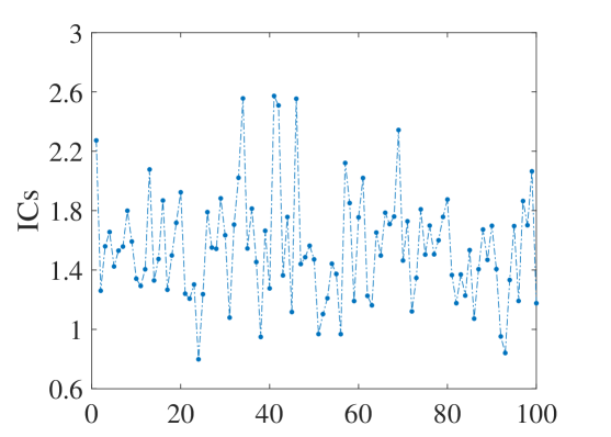
We performed a large number of numerical experiments to calculate the information content upper bound of the quantum system. We selected 100 random pure states, 50 random tensor product pure states, and 50 randomly rotated Bell states. Then the information content they contain is calculated respectively. The results of the numerical experiment on 2-qubit are shown in Fig. 1.

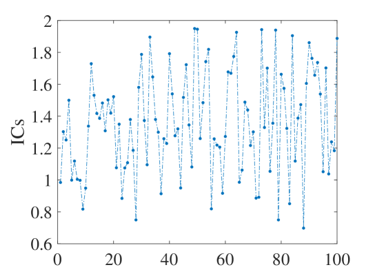
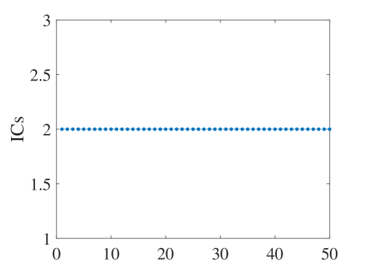
Refer to caption — (a) Information content of random pure states

Numerical experiments calculate the information content according to natural index order. In Fig.1, we can see that any state of different categories is consistent with the conclusion in Theorem 1. In particular, in Fig.1(b) we can see that when the system is a tensor product state, its information content is exactly equal to 2. At this time, the calculation result corresponds to the situation in the lemma 4.

Bell states serve as a typical example of quantum entanglement. We randomly select one of the four Bell states for calculation and the result is shown in Fig.1(c), and its information amount is exactly equal to 2. This corresponds to the situation in Lemma 3.

In the case of the 3-qubit quantum system, we also selected 100 random pure states, 50 random tensor product states and 50 random rotated three-valued Greenberger-Horne-Zeilinger (GHZ) states. The results of the numerical experiment are shown in Fig.2.

Comparing the case of 2-qubit systems, we obtained similar conclusions. In other words, the total amount of information contained in random quantum pure states is no more than 3 (that is shown in Fig.2(a)). When the selected state is a tensor product state or a 3-qubit GHZ state, we can always accurately obtain that the system information amount is exactly equal to 3 (shown in Fig.2(b) and 2(c)).

In fact, we have done many sets of numerical experiments, and have also done numerical experiments on 4-qubit systems and 5-qubit systems, all of which have given the same conclusion. Based on the conclusion given by the proposition 1, we generalized the Hypothesis 1 to $n$ -qubit system.

V Conclusion and outlook

We analyzes the posterior information and gives the information entropy contained in the parameters of the quantum state from a information divergence perspective. Based on the structural constraints of the quantum state, we obtained the upper bound of the posterior information content of the 2-qubit system, which is exactly equal to 2. And the hypothesis is extended to the $n$ -qubit system through the SDP proposition expressed by Bloch representation and numerical experiments: The posterior information content upper bound of $n$ -qubit system is $n$ (Hypothesis 1).

The work of this paper provides an important theoretical evidence for clarifying the consistency of classical systems and quantum systems in the information sense. If one similarly defines the posterior information of a classical bit system, in the same way as in the quantum case, the amount of a posterior information for $n$ classical bits is also precisely equal to $n$ . This is an elegant consistency. The posterior information upper bound hypothesis (Hypothesis 1) explicitly shows that the composite system constructed by quantum theory can ensure that the information carrying capacity will not lose control due to the nonlinear increase of parameters. The composite quantum system as an information carrying carrier can still comply with the basic constraints of information processing principles.

Especially in the realm of quantum state tomography, we noticed that hypothesis 1 has very striking connection with the work done by Huang et al., whose work related the classical and quantum worlds [14]. They present an efficient method named ”classical shadow”, which shows that $M$ functions defined on the quantum state can be accurately predicted with a very high probability of success only using measurements of order $O(\log M)$ , regardless of the dimensions of the quantum state. From the mathematical perspective, Huang’s method determines $M$ scalar parameters (i.e. the functions mentioned above) with measurements of order $O(\log M)$ . When $M=2^{n}$ , determining $M$ parameters requires at most $O(n)$ measurements. In this sense, a connection is established between the posterior information upper bound analysis and Huang’s work. (i.e. completely determining the density operator (containing $2^{n}$ scalar parameters) of an $n$ -dimensional quantum system requires at most $n$ classical bits.)

The posterior information upper bound hypothesis provides Huang’s work with clear theoretical evidence in terms of the information content of quantum states. The upper bound on the information content contained in a quantum state is also in principle the lower bound on an operational information theory of the quantum state. In other words, for an $n$ -qubit quantum state, at least $n$ measurements are required if this state is to be estimated by various methods. Similar to determining the state of a 2-qubit system, only at most 2 classical bits of information are needed. Therefore, for any 2-qubit quantum state $\psi$ clearly satisfies the numerical conclusion obtained by Huang’s work. In summary, the posterior information upper bound hypothesis gives a lower bound on the minimum number of normalized local measurements required to estimate the state of a quantum system. Its function is similar to the upper bound on the communication ratio of the noisy channel given by the Shannon–Hartley theorem [4].

More broadly, by analyzing the (classical) posterior information content contained in composite quantum systems, the posterior information upper bound hypothesis will provide perspectives and methods to analyze many challenging problems linking the relationship between the classical world and the quantum world. We think this will also be an inspiration for quantum information and quantum computing.

Acknowledgements.

This work is funded in part by the National Natural Science Foundation of China (61876129) and the European Unions Horizon 2020 research and innovation programme under the Marie Skodowska-Curie grant agreement No. 721321.

Appendix A The general form of a quantum pure state in Bloch representation

The Bloch formalization is equivalent to the density operator formalization, and its advantage is that it provides a more geometrically intuitive representation in low-dimensional cases and can more conveniently represent and analyze quantum correlations. The definition of the Bloch representation relies on the observables derived from a specific benchmark measurement. Typically, for a quantum bit, the following three Pauli observables (matrices) can be used:

\sigma_{1}=\begin{pmatrix}0&1\\ 1&0\end{pmatrix}\quad\sigma_{2}=\begin{pmatrix}0&-i\\ i&0\end{pmatrix}\quad\sigma_{3}=\begin{pmatrix}1&0\\ 0&-1\end{pmatrix}

(38)

For any 2-qubit composite system, if its density operator is expressed as $\rho$ , then its Bloch representation can be expressed as $\ \psi=(\bm{\alpha},\bm{\beta},C)$ . Among them, $\bm{\alpha}$ and $\bm{\beta}$ are

\bm{\alpha}=\begin{pmatrix}\operatorname{tr}((\sigma_{1}\otimes I)\rho)\\ \operatorname{tr}((\sigma_{2}\otimes I)\rho)\\ \operatorname{tr}((\sigma_{3}\otimes I)\rho)\end{pmatrix},\bm{\beta}=\begin{pmatrix}\operatorname{tr}((I\otimes\sigma_{1})\rho)\\ \operatorname{tr}((I\otimes\sigma_{2})\rho)\\ \operatorname{tr}((I\otimes\sigma_{3})\rho)\end{pmatrix}

(39)

and $C$ is a 3 × 3 correlation matrix defined as

C=\begin{pmatrix}\operatorname{tr}((\sigma_{1}\otimes\sigma_{1})\rho)&\operatorname{tr}((\sigma_{1}\otimes\sigma_{2})\rho)&\operatorname{tr}((\sigma_{1}\otimes\sigma_{3})\rho)\\ \operatorname{tr}((\sigma_{2}\otimes\sigma_{1})\rho)&\operatorname{tr}((\sigma_{2}\otimes\sigma_{2})\rho)&\operatorname{tr}((\sigma_{2}\otimes\sigma_{3})\rho)\\ \operatorname{tr}((\sigma_{3}\otimes\sigma_{1})\rho)&\operatorname{tr}((\sigma_{3}\otimes\sigma_{2})\rho)&\operatorname{tr}((\sigma_{3}\otimes\sigma_{3})\rho)\end{pmatrix}

(40)

In Bloch representation, the elements in $\alpha$ are usually defined as $b_{2}-b_{4}$ , the elements in $\beta$ are defined as $b_{5}-b_{7}$ , and the elements in $C$ are defined as $b_{8}-b_{16}$ in row-major order. In addition, $b_{1}=\operatorname{tr}((I\otimes I)\rho)=1$ .

For the detailed proof of Eq.1-3 in the main text, please refer to the Ref.[18]. We only give a general idea. There are unitary transformations between any pure states that allow them to be converted to each other, which means that all pure states can be generated through unitary transformations based on direct product states. In addition, local transformations do not change the form of the diagonal matrix of $C$ after SVD decomposition. This diagonal matrix can only be controlled by non-local transformations. Non-local transformations have the following general form:

\tilde{U}(\theta_{1},\theta_{2},\theta_{3})=\tilde{U}_{1}(\theta_{1})\tilde{U}_{2}(\theta_{2})\tilde{U}_{3}(\theta_{3})

(41)

where

\tilde{U}_{j}(\theta_{j})=\exp\left(\frac{\theta_{j}}{2}\sigma_{j}\otimes\sigma_{j}\right)

(42)

Acting on the pure state of the direct product of $\bm{\alpha}=(1,0,0)^{\mathrm{T}}$ and $\bm{\beta}=(1,0,0)^{\mathrm{T}}$ , we can obtain

\bm{\alpha}=\begin{pmatrix}\cos\theta\\ 0\\ 0\end{pmatrix},\bm{\beta}=\begin{pmatrix}\cos\theta\\ 0\\ 0\end{pmatrix},C=\left(\begin{array}[]{ccc}1&0&0\\ 0&0&\sin\theta\\ 0&\sin\theta&0\end{array}\right)

(43)

where $\theta=\theta_{2}-\theta_{3}$ .

Note that for the sake of discussion, the form of the pure state given by Eq.1-3 is not consistent with the form given by Eq.43. In fact, as long as the parameters in $O_{1}$ and $O_{2}$ are represented as:

\sin\omega=-1,\cos\varphi=1,\cos k=1

(44)

It gets the same form as in Eq.1-3.

On this basis, we can calculate that:

\alpha=\left(\begin{array}[]{c}\cos\theta\cos\phi\cos k\\ -\cos\theta\cos\phi\sin k\\ \cos\theta\sin\phi\\ \end{array}\right)\\ ,\beta=\left(\begin{array}[]{c}\cos\theta\cos\phi^{\prime}\cos k^{\prime}\\ -\cos\theta\cos\phi^{\prime}\sin k^{\prime}\\ \cos\theta\sin\phi^{\prime}\end{array}\right)

(45)

In particular, when $\cos\theta=0$ , $\bm{a},\bm{b}=\bm{0}$ . The parameters of the matrix C can be represented as:

\begin{split}c_{11}&=\cos\phi\cos k\cos\phi^{\prime}\cos k^{\prime}\\ &\quad+\sin\theta\left(\cos\omega\sin k+\sin\omega\sin\phi\cos k\right)\left(\cos\omega^{\prime}\sin k^{\prime}+\sin\omega^{\prime}\sin\phi^{\prime}\cos k^{\prime}\right)\\ &\quad-\sin\theta\left(\sin\omega\sin k-\cos\omega\sin\phi\cos k\right)\left(\sin\omega^{\prime}\sin k^{\prime}-\cos\omega^{\prime}\sin\phi^{\prime}\cos k^{\prime}\right)\\ &=\cos\phi\cos k\cos\phi^{\prime}\cos k^{\prime}\\ &\quad-\sin\theta\sqrt{1-\cos^{2}\phi\cos^{2}k}\sqrt{1-\cos^{2}\phi^{\prime}\cos^{2}k^{\prime}}\cos(\omega+\omega^{\prime}+\omega_{1}+\omega_{1}^{\prime})\end{split}

(46)

\begin{split}c_{12}&=-\cos\phi\cos k\cos\phi^{\prime}\sin k^{\prime}\\ &\quad+\sin\theta\left(\cos\omega\sin k+\sin\omega\sin\phi\cos k\right)\left(\cos\omega^{\prime}\cos k^{\prime}-\sin\omega^{\prime}\sin\phi^{\prime}\sin k^{\prime}\right)\\ &\quad-\sin\theta\left(\sin\omega\sin k-\cos\omega\sin\phi\cos k\right)\left(\sin\omega^{\prime}\cos k^{\prime}+\cos\omega^{\prime}\sin\phi^{\prime}\sin k^{\prime}\right)\\ &=-\cos\phi\cos k\cos\phi^{\prime}\sin k^{\prime}\\ &\quad+\sin\theta\sqrt{1-\cos^{2}\phi\cos^{2}k}\sqrt{1-\cos^{2}\phi^{\prime}\sin^{2}k^{\prime}}\sin(\omega+\omega^{\prime}+\omega_{1}+\omega_{2}^{\prime})\end{split}

(47)

where

		$\displaystyle\sin\omega_{1}=\frac{\sin k}{\sqrt{\sin^{2}k+\sin^{2}\phi\cos^{2}k}},\sin\omega_{1}^{{}^{\prime}}=\frac{\sin k^{{}^{\prime}}}{\sqrt{\sin^{2}k+\sin^{2}\phi^{{}^{\prime}}\cos^{2}k^{{}^{\prime}}}},\sin\omega_{2}^{{}^{\prime}}=\frac{\cos k^{{}^{\prime}}}{\sqrt{\cos^{2}k^{{}^{\prime}}+\sin^{2}\phi^{{}^{\prime}}\sin^{2}k^{{}^{\prime}}}}$		(48)
		$\displaystyle\cos\omega_{1}=\frac{\sin\phi\text{cos}k}{\sqrt{\sin^{2}k+\sin^{2}\phi\text{cos}^{2}k}},\cos\omega_{1}^{{}^{\prime}}=\frac{\sin\phi^{{}^{\prime}}\cos k^{{}^{\prime}}}{\sqrt{\sin^{2}k^{{}^{\prime}}+\sin^{2}\phi^{{}^{\prime}}\cos^{2}k^{{}^{\prime}}}},\cos\omega_{2}^{{}^{\prime}}=\frac{\sin\phi^{{}^{\prime}}\sin k^{{}^{\prime}}}{\sqrt{\cos^{2}k^{{}^{\prime}}+\sin^{2}\phi^{{}^{\prime}}\sin^{2}k^{{}^{\prime}}}}$		(48)

Appendix B The prior information of 2-qubit pure state

In order to clarify the information signification of pure state 2-quantum system, we will give a specific definition of prior information. For the pure state 2-qubit Bloch vector represented by Eq.4, its prior $\chi^{2}$ distance information is defined as:

I_{\chi^{2},prior}(\psi)=\sum_{i=2}^{16}D_{\chi^{2}}(\psi_{i},\mu_{2,2})

(49)

where $\mu_{2,2}$ is comparison benchmark of the prior $\chi^{2}$ distance information content [22].

Appendix C Pythagorean properties of $\chi^{2}$ divergence

Lemma 1 (Pythagorean properties).

Assume that $t_{1}$ , $t_{2}$ , $t_{3}$ are components of the Bloch vector, and $t_{1}^{2}=t_{2}^{2}+t_{3}^{2}$ . then:

D_{X^{2}}(t_{1},0)\equiv D_{X^{2}}(t_{2},0)+D_{X^{2}}(t_{3},0)

(50)

Proof.

From the relationship between probability and Bloch parameters, It can be given:

$\displaystyle D_{X^{2}}(t_{1},0)$	$\displaystyle=\frac{(\frac{t_{1}+1}{2})^{2}}{\frac{1}{2}}+\frac{(\frac{1-t_{1}}{2})^{2}}{\frac{1}{2}}-1$	(51)
	$\displaystyle=\frac{(t_{1}+1)^{2}}{2}+\frac{(1-t_{1})^{2}}{2}-1$
	$\displaystyle=\frac{t_{1}^{2}+2t_{1}+1}{2}+\frac{t_{1}^{2}-2t_{1}+1}{2}-1$
	$\displaystyle=t_{1}^{2}$

In the same way, the above calculation can be performed for $t_{2}$ and $t_{3}$ , and the lemma is proved. ∎

Appendix D The unique determination of pure states in 2-qubit systems

The Bloch representation of a quantum pure state involves many parameters and they are coupled to each other. This is not conducive to analyze information content. First notice, $\omega+\omega^{\prime}$ can be discussed as a whole parameter without discussing the values of $\omega$ and $\omega^{\prime}$ separately. then, We derive the following lemma.

Lemma 2 (Unique determination).

Proof.

Given $\bm{\alpha}$ and $\bm{\beta}$ ( $\cos{\theta}\geq 0$ ), then $\sin{\phi}$ and $\sin{\phi}^{\prime}$ can be uniquely determined, but the signs of the remaining trigonometric function values in $\bm{\alpha}$ and $\bm{\beta}$ cannot be uniquely determined. We can assume that $\cos\phi,\cos k,\sin k$ and $\cos\phi^{\prime},\cos k^{\prime},\sin k^{\prime}$ satisfy the constant value requirements of $\bm{\alpha}$ and $\bm{\beta}$ . Then $-\cos\phi,-\cos k,-\sin k$ and $-\cos\phi^{\prime},-\cos k^{\prime},-\sin k^{\prime}$ also satisfy requirements of $\bm{\alpha}$ and $\bm{\beta}$ . In other words, if $\phi,k$ and $\phi^{\prime},k^{\prime}$ satisfy the requirements, $\pi-\phi,\pi+k$ and $\pi-\phi^{\prime},\pi+k^{\prime}$ also satisfy the requirements without considering the period. Now, there are four sets of satisfying angles: $(\phi,k,\phi^{\prime},k^{\prime})$ , $(\pi-\phi,\pi+k,\phi^{\prime},k^{\prime}),(\phi,k,\pi-\phi^{\prime},\pi+k^{\prime})$ , and $(\pi-\phi,\pi+k,\pi-\phi^{\prime},\pi+k^{\prime})$ .

Next, we analyse the values of $c_{11}$ and $c_{12}$ . Assume that the current value of $\omega+\omega^{\prime}$ makes $c_{11}$ and $c_{12}$ the aforementioned constant values. According to the above analysis, the current values of the angle parameters are changed from $(\phi,k,\phi^{\prime},k^{\prime})$ to $(\pi-\phi,\pi+k,\phi^{\prime},k^{\prime})$ or $(\phi,k,\pi-\phi^{\prime},\pi+k^{\prime})$ , the values of $\bm{\alpha}$ and $\bm{\beta}$ remain unchanged. Correspondingly, when the above changes occur, the value of $\omega_{1}+\omega_{1}^{\prime}(\omega_{1}+\omega_{2}^{\prime})$ will become $\omega_{1}+\omega_{1}^{\prime}+\pi(\omega_{1}+\omega_{2}^{\prime}+\pi)$ within one cycle. At this time, the current values of $\omega$ and $\omega^{\prime}$ will no longer be able to keep $c_{11}$ and $c_{12}$ at constant values, and $\omega+\omega^{\prime}$ can only be modified to $\omega+\omega^{\prime}+\pi$ . By the same token, when $(\phi,k,\phi^{\prime},k^{\prime})$ changes into $(\pi-\phi,\pi+k,\pi-\phi^{\prime},\pi+k^{\prime})$ , to keep $c_{11}$ and $c_{12}$ as constant values, $\omega+\omega^{\prime}$ should be modified to $\omega+\omega^{\prime}+2\pi$ .

In summary, the same values of $\bm{\alpha}$ , $\bm{\beta}$ , $c_{11}$ and $c_{12}$ can be obtained at the same time for only the following four sets of rotated matrix angle with ignoring the cycles:

		$\displaystyle\left(\mathrm{a}\right)\phi,k,\phi^{\prime},k,\omega+\omega^{\prime}$		(52)
		$\displaystyle\left(\mathrm{b}\right)\pi-\phi,\pi+k,\phi^{\prime},k^{\prime},\omega+\omega^{\prime}+\pi$
		$\displaystyle\left(\mathrm{c}\right)\phi,k,\pi-\phi^{\prime},\pi+k^{\prime},\omega+\omega^{\prime}+\pi$
		$\displaystyle\left(\mathrm{d}\right)\pi-\phi,\pi+k,\pi-\phi^{\prime},\pi+k^{\prime},\omega+\omega^{\prime}+2\pi$

By calculating $\bm{C}$ through these four sets of values, it can be seen that $\bm{C}$ will not change. In other words, it can be considered that the trigonometric function values of $\phi$ , $k$ , $\phi^{\prime}$ , $k^{\prime}$ (including their signs) are determined(i.e. quantum state is uniquely determined), after given $\bm{\alpha}$ , $\bm{\beta}$ , $c_{11}$ and $c_{12}$ .

∎

Therefore, when $\cos^{2}\phi\cos^{2}k\neq 0$ or $\cos^{2}\phi^{\prime}\cos^{2}k^{\prime}\neq 0$ , to calculate the information content of a quantum state under the constraints of the pure state structure, only need to calculate the information contained in $\bm{\alpha}$ , $\bm{\beta}$ , $c_{11}$ and $c_{12}$ . More detailed analysis can be found in [23].

Appendix E The proof of proposition 1

We redescribe Proposition.1 in Section IV.

Proposition 1.

For any positive integer $n$ , any (standard) $n$ -qubit system, its first $k-1$ parameters $b_{i},\;1\leq i\leq k-1\leq{4^{n}}$ are given in the natural index order of the standard Bloch representation. Assume ${b_{k}}$ is the $k$ -th parameter, then the upper bound $U_{b_{k}}$ and the lower bound $L_{b_{k}}$ of parameter ${b_{k}}$ can be solved by the standard SDP.

•

For the lower bound problem:

$\begin{array}[]{rl}\min\limits&{b_{k}}\\ \text{subject to}&-1\leq{b_{k}},\cdots,{b_{{4^{n}}}}\leq 1\\ &Q\succeq 0\end{array}$ (53)

•

For the upper bound problem:

$\begin{array}[]{rl}\min\limits&{-b_{k}}\\ \text{subject to}&-1\leq{b_{k}},\cdots,{b_{{4^{n}}}}\leq 1\\ &Q\succeq 0\end{array}$ (54)

Proof.

According to the standard form of the SDP problem as follows:

\begin{array}[]{rl}\min\limits_{X\in S^{2^{n}}}&\langle C,X\rangle_{\mathbb{S}^{2^{n}}}\\ \text{subject to}&\langle A_{i},X\rangle_{\mathbb{S}^{2^{n}}}\leq d_{i},\\ &X\succeq 0\end{array}

(55)

If the above proposition is true, the objective function needs to satisfy $\langle C,Q\rangle=b_{k}$ , and the constraints need to satisfy $-1\leq\langle A_{i},Q\rangle=b_{i}\leq 1$ , $i\in[k,4^{n}]$ .

Therefore, it is only necessary to prove that for each $b_{k}$ corresponds to a matrix $C$ and a set of $A_{k}$ , and they are all Hermitian matrix, and make the formalization of Eq.(53) and (54) can be obtained.

In a $n$ -qubit composite system, the Bloch parameter $b_{k}$ can be determined from local fiducial measurements. Its measurement process can be expressed as:

\langle A_{k},Q\rangle=b_{k}

(56)

Where $A_{k}$ is a the measurement operator, and each Bloch parameter corresponds to a measurement operator $A_{k}$ . For example, taking the seventh parameter $b_{7}$ in the 2-qubit quantum system as an example, the measurement operator $A_{7}$ corresponding to the seventh parameter $b_{7}$ is ${\sigma_{1}}\otimes{\sigma_{1}}$ , and its matrix is expressed as

{\sigma_{1}}\otimes{\sigma_{1}}=\left[{\begin{array}[]{*{20}{c}}0&0&0&1\\ 0&0&1&0\\ 0&1&0&0\\ 1&0&0&0\end{array}}\right]

(57)

Because $A_{k}$ is a tensor matrix composed of ${\sigma_{i}},i\in\left\{{0,1,2,3}\right\}$ , it must be a Hermitian matrix.

When the $k$ -th Bloch parameter $b_{k}$ is calculated, it is obvious that the matrix $C$ should be equal to the measurement operator $A_{k}$ of $b_{k}$ .

Therefore, there is always a set of identical matrix $C$ and $A_{k}$ corresponding to each Bloch parameter $b_{k}$ , making the process of calculating the upper and lower bounds of the posterior information (Eq.(53) and (54)) into a standard SDP. ∎

The above proposition shows that even in a high-dimensional qubit space $(n>2)$ , the process of calculating the upper bound of the posterior information amount can always be analogized to the situation of solving the 2-qubit space, and it can be summarized as an SDP problem.

References

Heisenberg and Bohr [1958] W. Heisenberg and N. Bohr, Copenhagen interpretation, Physics and philosophy (1958).
Wheeler [2018] J. A. Wheeler, Information, physics, quantum: The search for links, Feynman and computation , 309 (2018).
Nielsen and Chuang [2010] M. A. Nielsen and I. L. Chuang, Quantum computation and quantum information (Cambridge university press, 2010).
Shannon [1948] C. E. Shannon, A mathematical theory of communication, The Bell system technical journal 27, 379 (1948).
Bengtsson and Życzkowski [2017] I. Bengtsson and K. Życzkowski, Geometry of quantum states: an introduction to quantum entanglement (Cambridge university press, 2017).
Banchi et al. [2021] L. Banchi, J. Pereira, and S. Pirandola, Generalization in quantum machine learning: A quantum information standpoint, PRX Quantum 2, 040321 (2021).
Ingarden et al. [2013] R. S. Ingarden, A. Kossakowski, and M. Ohya, Information dynamics and open systems: classical and quantum approach, Vol. 86 (Springer Science & Business Media, 2013).
Brydges et al. [2019] T. Brydges, A. Elben, P. Jurcevic, B. Vermersch, C. Maier, B. P. Lanyon, P. Zoller, R. Blatt, and C. F. Roos, Probing rényi entanglement entropy via randomized measurements, Science 364, 260 (2019).
Elben et al. [2019] A. Elben, B. Vermersch, C. F. Roos, and P. Zoller, Statistical correlations between locally randomized measurements: A toolbox for probing entanglement in many-body quantum states, Physical Review A 99, 052323 (2019).
Kalev et al. [2015] A. Kalev, R. L. Kosut, and I. H. Deutsch, Quantum tomography protocols with positivity are compressed sensing protocols, npj Quantum Information 1, 1 (2015).
Lloyd et al. [2014] S. Lloyd, M. Mohseni, and P. Rebentrost, Quantum principal component analysis, Nature Physics 10, 631 (2014).
Cavalcanti et al. [2022] P. J. Cavalcanti, J. H. Selby, J. Sikora, T. D. Galley, and A. B. Sainz, Post-quantum steering is a stronger-than-quantum resource for information processing, npj Quantum Information 8, 76 (2022).
Aaronson [2018] S. Aaronson, Shadow tomography of quantum states, in Proceedings of the 50th annual ACM SIGACT symposium on theory of computing (2018) pp. 325–338.
Huang et al. [2020] H.-Y. Huang, R. Kueng, and J. Preskill, Predicting many properties of a quantum system from very few measurements, Nature Physics 16, 1050 (2020).
Huang et al. [2021a] H.-Y. Huang, M. Broughton, M. Mohseni, R. Babbush, S. Boixo, H. Neven, and J. R. McClean, Power of data in quantum machine learning, Nature Communications 12, 2631 (2021a).
Lewis et al. [2023] L. Lewis, H.-Y. Huang, V. T. Tran, S. Lehner, R. Kueng, and J. Preskill, Improved machine learning algorithm for predicting ground state properties, arXiv preprint arXiv:2301.13169 (2023).
Huang et al. [2023] H.-Y. Huang, S. Chen, and J. Preskill, Learning to predict arbitrary quantum processes, PRX Quantum 4, 040337 (2023).
Gamel [2016] O. Gamel, Entangled bloch spheres: Bloch matrix and two-qubit state space, Physical Review A 93, 062320 (2016).
Rényi [1961] A. Rényi, On measures of entropy and information, in Proceedings of the Fourth Berkeley Symposium on Mathematical Statistics and Probability, Volume 1: Contributions to the Theory of Statistics, Vol. 4 (University of California Press, 1961) pp. 547–562.
Popescu et al. [2016] P. G. Popescu, S. S. Dragomir, E. I. Sluşanschi, and O. N. Stănăşilă, Bounds for kullback-leibler divergence, Electronic Journal of Differential Equations 2016 (2016).
Dragomir [2002] S. Dragomir, Upper and lower bounds for csiszár f-divergence in terms of hellinger discrimination and applications, in Nonlinear Analysis Forum, Vol. 7 (2002) pp. 1–14.
Masanes and Müller [2011] L. Masanes and M. P. Müller, A derivation of quantum theory from physical requirements, New Journal of Physics 13, 063001 (2011).
Zhang [2022] C. Zhang, The Application of Quantum-like Mechanisms in Pattern Recognition and Model Selection(in Chinese), Ph.D. thesis, College of Intelligence and Computing, Tianjin University, Tianjin (2022).
Wehrl [1979] A. Wehrl, On the relation between classical and quantum-mechanical entropy, Reports on Mathematical Physics 16, 353 (1979).
Floerchinger et al. [2022] S. Floerchinger, M. Gärttner, T. Haas, and O. R. Stockdale, Entropic entanglement criteria in phase space, Physical Review A 105, 012409 (2022).
Abanin et al. [2019] D. A. Abanin, E. Altman, I. Bloch, and M. Serbyn, Colloquium: Many-body localization, thermalization, and entanglement, Reviews of Modern Physics 91, 021001 (2019).
Huang et al. [2021b] S. Huang, Z.-B. Chen, and S. Wu, Entropic uncertainty relations for general symmetric informationally complete positive operator-valued measures and mutually unbiased measurements, Physical Review A 103, 042205 (2021b).
Takakura and Miyadera [2021] R. Takakura and T. Miyadera, Entropic uncertainty relations in a class of generalized probabilistic theories, Journal of Physics A: Mathematical and Theoretical 54, 315302 (2021).
Jevtic et al. [2014] S. Jevtic, M. Pusey, D. Jennings, and T. Rudolph, Quantum steering ellipsoids, Phys. Rev. Lett. 113, 020402 (2014).
Wehrl [1978] A. Wehrl, General properties of entropy, Reviews of Modern Physics 50, 221 (1978).
Nielsen [2000] M. A. Nielsen, Quantum information theory (2000), arXiv:quant-ph/0011036 [quant-ph] .

Information upper bounds in composite quantum systems

Abstract

I introduction

II PRELIMINARIES

II.1 General representation of 2-qubit pure states

II.2 Information divergence

Definition 1 (χ2\chi^{2} distance information content).

III The information upper bound of pure state in 2-qubit system

Definition 2 (The posterior χ2\chi^{2} divergence information content).

Remark.

Lemma 1 (Pythagorean properties).

Proof.

Lemma 2 (Unique determination).

Proof.

Lemma 3.

Proof.

Lemma 4.

Proof.

Lemma 5.

Proof.

Theorem 1.

IV The information upper bound of pure state in n-qubit system

Hypothesis 1 (The posterior information content upper bound).

Proposition 1 (Semi-definite Programming).

Remark.

Remark.

Proof.

V Conclusion and outlook

Acknowledgements.

Appendix A The general form of a quantum pure state in Bloch representation

Appendix B The prior information of 2-qubit pure state

Appendix C Pythagorean properties of χ2\chi^{2} divergence

Lemma 1 (Pythagorean properties).

Proof.

Appendix D The unique determination of pure states in 2-qubit systems

Lemma 2 (Unique determination).

Proof.

Appendix E The proof of proposition 1

Proposition 1.

Proof.

References

Definition 1 ( $\chi^{2}$ distance information content).

Definition 2 (The posterior $\chi^{2}$ divergence information content).

Appendix C Pythagorean properties of $\chi^{2}$ divergence