Influence Maximization in Hypergraphs
Abstract
Influence maximization in complex networks, i.e., maximizing the size of influenced nodes via selecting seed nodes for a given spreading process, has attracted great attention in recent years. However, the influence maximization problem in hypergraphs, in which the hyperedges are leveraged to represent the interactions among more than two nodes, is still an open question. In this paper, we propose an adaptive degree-based heuristic algorithm, i.e., Heuristic Degree Discount (HDD), which iteratively selects nodes with low influence overlap as seeds, to solve the influence maximization problem in hypergraphs. We further extend algorithms from ordinary networks as baselines and compare the performance of the proposed algorithm and baselines on both real data and synthetic hypergraphs. Results show that HDD outperforms the baselines in terms of both effectiveness and efficiency. Moreover, the experiments on synthetic hypergraphs indicate that HDD shows high performance especially in hypergraphs with heterogeneous degree distribution.
keywords:
complex networks , influence maximization , hypergraphs , spreading dynamics1 Introduction
As a classical optimization problem, influence maximization aims to find a set of initial spreaders that maximize the influence spread under a certain spreading dynamics in a network. Due to its abundant applications, e.g., the control of disease [1], the dissemination of information [2, 3] and viral marketing [4, 5], the problem is widely studied in recent years. Extensive researches of influence maximization are oriented to ordinary networks, where nodes represent individuals and edges represent pairwise interactions between individuals. The problem was first proposed to identify the most helpful customers in viral marketing [4]. Later on, Kempe et al. [6] used two popular diffusion models, Independent Cascade model and Linear Threshold model, in influence maximization. They modeled this problem as a combinatorial optimization problem, which is proved to be NP-hard, and proposed a greedy algorithm which can guarantee a approximation ratio for selecting the seed nodes to tackle it. In addition, the cost effective lazy forward method (CELF [7]) and its improved variant (CELF++ [8]) were designed respectively to improve the efficiency of the greedy algorithm. Moreover, there are many other methods proposed to improve the efficiency and the accuracy of influence maximization[9, 10, 11, 12], including maximum influence arborescence (MIA) [5], Prefix excluding MIA (PMIA) [13] and Two-phase Influence Maximization (TIM) [14].
In many real-world scenarios, an edge in ordinary networks with dyadic relationship could hardly characterize the interactions if the interactions involve more than two entities. For example, many users could form groups for information sharing in social platforms, more than two researchers may contribute to one scientific paper, and many people might be listed in mass emails. This kind of relations could be represented by a hypergraph [15, 16, 17], with hyperedges characterizing the polyadic interactions among more than two nodes [18]. In light of influence maximization in hypergraphs, it is still a mostly unexplored problem with only a few studies focusing on this field. For instance, Amato et al. [19] modelled the social media network via a hypergraph, in which user-to-multimedia relationships are represented by hyperedges. They further applied algorithms, such as TIM+ [14] and IMM [20], which were proposed to solve influence maximization problem in bipartite graphs, to tackle the influence maximization in a hypergraph after transforming it to a bipartite graph. Zhu et al.[21] proved that influence maximization in directed hypergraphs under independent cascade model is a NP-hard problem and designed a sandwich framework which provides a approximation ratio with high computational complexity to solve it. A ranking-based algorithm was proposed to solve the influence maximization problem under the HyperCascade model [22], where the model actually considers spreading process on the bipartite augment graph of a hypergraph. In addition, a set of greedy-based heuristic strategies were proposed to solve the minimum target set selection problem in hypergraphs [23]. However, the above researches either considered to transform hypergraphs to bipartite graphs or designed greedy algorithms to solve the influence maximization problem in hypergraphs, ignoring the basic hypergraph topological structures which may play a crucial role in solving the influence maximization problem. In this paper, we aim to explore how to utilize the basic topological properties of a hypergraph for influence maximization.
Degree centrality, as an essential topological property, was frequently used to characterize the node importance in a network [24, 25]. In this paper, we address the problem of how to choose the initial seeds for influence maximization in hypergraphs based on the node degree. Firstly, we design a discrete-time susceptible-infected (SI) model with Contact Process (CP) [26] to model the influence spreading process in hypergraphs. Then, we propose Heuristic Degree Discount (HDD) algorithm for influence maximization, which iteratively avoids choosing nodes that have large influence overlap with the existing seeds as the seed candidates. Experiments indicate that the proposed algorithm can achieve better performance efficiently and accurately compared with the baselines on both real-world data and synthetic hypergraphs.
The remainder of this paper is organized as follows. Section 2 presents preliminary definitions of a hypergraph and the description of real-world data. In Section 3, we illustrate the influence maximization problem in hypergraphs, the spreading model as well as the algorithms. Experimental results and analysis are given in Section 4. Finally, we conclude the paper in Section 5.
2 Representation of a Hypergraph
2.1 Definition of a Hypergraph
A hypergraph is represented as , in which is the node set and is the hyperedge set. An incidence matrix of is given by , where
| (1) |
Therefore, the adjacency matrix can be derived from ,
| (2) |
where is a diagonal matrix whose diagonal elements represent the number of hyperedges a node belongs to. The value of indicates the number of hyperedges that contain both node and node . An example of a hypergraph is given in Figure 1, which contains 5 nodes and 2 hyperedges. The incidence matrix and adjacency matrix are also given correspondingly.

Given the incidence matrix of a hypergraph, we can define the degree of a node in a hypergraph in two different ways [27], i.e., the degree and the hyperdegree. The degree of a node () indicates the number of neighboring nodes that is adjacent to, which can be expressed as follows:
| (3) |
where
| (4) |
The hyperdegree of node is defined as the number of hyperedges that node belongs to, which is given by the following equation:
| (5) |
According to the above definitions, we can calculate the degree and hyperdegree of the nodes in Figure 1. For instance, the degree of node is and the hyperdegree of node is .
2.2 Data description
We show the basic description and properties of eight hypergraphs generated by real-world datasets, which are collected from different domains111https://www.cs.cornell.edu/~arb/data/ 222http://bigg.ucsd.edu/. The hypergraphs will be used to evaluate the performance of our algorithms in the subsequent sections. The topological properties of them are given in Table 1. The detailed description of each data is given as follows:
cat-edge-algebra-questions dataset (Algebra) & cat-edge-geometry-questions dataset (Geometry). The two datasets contain interactions between users on the stack exchange web site Math Overflow. The interactions between users are mainly about comments, questions and answers on algebra (or geometry) problems. Each node represents a user on MathOverflow and hyperedges are sets of users who answered a certain question category (algebra or geometry).
cat-edge-madison-restaurant-reviews (Restaurant-Rev). The data indicates users who reviewed an establishment of a particular category (different types of restaurants in Madison, WI) within a month timeframe. Each node represents a user on Yelp and a hyperedge represents a set of users who reviewed a certain restaurant.
cat-edge-music-blues-reviews (Music-Rev). The data contains nodes representing users on Amazon, and hyperedges are sets of reviewers who reviewed a certain product category (different types of blues music) within a month timeframe.
cat-edge-vegas-bars-reviews (Bars-Rev). Each node in the dataset represents a user on Yelp, and a hyperedge is a set of users who reviewed a certain bar in Las Vegas, NV.
NDC-classes. The dataset contains nodes representing class labels, and a hyperedge is a drug which consists of a set of class labels.
iAF1260b. The data contains nodes representing reaction-based metabolics, and hyperedges are sets of metabolics which are applied to a certain reaction. The duplicate hyperedges are removed.
iJO1366. Similar to iAF1260b, this is also a metabolic hypergraph with each node representing a reaction-based metabolic, and hyperedges are sets of metabolics which are applied to a certain reaction. The duplicate hyperedges are removed.
| Data | |||||||||
|---|---|---|---|---|---|---|---|---|---|
| Algebra | 423 | 1268 | 78.90 | 19.53 | 6.52 | 0.79 | 1.95 | 5 | 0.19 |
| Restaurant-Rev | 565 | 601 | 79.75 | 8.14 | 7.66 | 0.54 | 1.98 | 5 | 0.14 |
| Geometry | 580 | 1193 | 164.79 | 21.53 | 10.47 | 0.82 | 1.75 | 4 | 0.28 |
| Music-Rev | 1106 | 694 | 167.87 | 9.49 | 15.13 | 0.62 | 1.99 | 8 | 0.15 |
| NDC-classes | 1161 | 1088 | 10.71 | 5.55 | 5.92 | 0.61 | 3.50 | 9 | 0.01 |
| Bars-Rev | 1234 | 1194 | 174.30 | 9.61 | 9.93 | 0.58 | 2.10 | 6 | 0.14 |
| iAF1260b | 1668 | 2351 | 13.26 | 5.46 | 3.87 | 0.55 | 2.67 | 7 | 0.007 |
| iJO1366 | 1805 | 2546 | 16.91 | 5.55 | 3.94 | 0.58 | 2.62 | 7 | 0.009 |
3 Models and Algorithms
3.1 Problem statement
Given a specific spreading model, the influence maximization problem[28] aims to identify spreaders (also called seed nodes) in a network that can maximize the expected number of influenced nodes. Mathematically, the problem can be described as follows,
| (6) |
where represents the expected influence of the seed node set , and the number of nodes in the seed set is the constraint condition of this problem.
It has been shown that the influence maximization problem in ordinary networks is NP-hard [6]. And the influence maximization problem in hypergraphs, which can be considered as the generalization of influence maximization in ordinary networks, is also NP hard [21]. That is to say, it cannot be solved in polynomial time. Therefore, we propose to use greedy and heuristic algorithms to approximate its optimal solution.
3.2 SI spreading model with Contact Process dynamics
To quantify the spreading influence of the seed nodes [29, 30], we propose to use a Susceptible-Infected (SI) model with Contact Process (CP) dynamics on a hypergraph [26, 31]. In the model, an individual can only take one of the two states, i.e., susceptible (S) or infected (I). An S-state node can be infected by each of its I-state neighbors with infection probability . The model is described as follows:
(i) Initially, nodes in the seed set are set to be I-state and the rest nodes are in S-state.
(ii) At each time step , we first find the I-state nodes. For each I-state node , we find all the hyperedges that node belongs to. Then a hyperedge is chosen from uniformly at random. For each of the S-state nodes in , it will be infected by node with infection probability .
(iii) We terminate the process until a specific time step reaches, where is a control parameter.
We show an illustrative example of the spreading process in Figure 2. At time step , node is in I-state. The hyperedge set that contains is . At time step , the S-state nodes, i.e., and in hyperedge , are infected by node . Subsequently, the I-state nodes , and infect the S-state nodes in hyperedges .

3.3 Degree-based heuristic algorithms
Given nodes and , we suppose that the influenced node sets at time step by setting node and as the seed node are given by and , respectively. Thus, the influence overlap at time step between and can be defined as . In Figure 3, we show the comparison between the influence overlap distribution of a neighboring node pair and a randomly selected node pair in various hypergraphs. In most of the datasets (i.e., Figure 3(a), (b), (e), (g) and (h)), the probability that a neighboring node pair have overlapped influence is always higher than that of a randomly selected node pair. It suggests that when we choose one node as the seed, the probability that its neighboring nodes are choosing as the seed should be lower to avoid overlapped influence. Based on this assumption, we propose an adaptive degree-based heuristic algorithm, i.e., Heuristic Degree Discount (HDD), to solve the influence maximization problem.

Heuristic Degree Discount (HDD). In HDD, we aim to punish nodes that have more neighbors in in each iteration. The details of HDD is shown in Algorithm 1. To conduct the algorithm, we first give the original degree vector of all the nodes as .
(i) At the initial step, a node that has the largest degree is chosen, i.e., , and added to the seed set . For every neighboring node of , we first find the neighbors of in and collect them as a set . Then the adaptive degree of node is updated as , where is the number of elements in . For the other nodes that are not the neighbors of , e.g., node , . After updating the adaptive degree of every node, we obtain an adaptive degree vector .
(ii) At step , the node that has the largest adaptive degree (denoted as ), i.e., , is chosen, and we add it to the seed set . For every neighboring node of , we first find the neighbors of in and collect them as a set . The adaptive degree of is further updated by , where is the number of elements in . For the other nodes that are not the neighbors of , e.g., node , . We obtain a new adaptive degree vector as after updating the adaptive degree of every node.
(iii) The algorithm is terminated when we obtain seed nodes.
We propose a simplified algorithm which considers to give an even penalty for every node in the iteration, i.e., at step , the adaptive degree of is further updated by , where . The simplified algorithm is named as Heuristic Single Discount (HSD), which we will use as a baseline for comparison. We show the details of HSD in Algorithm 2.
3.4 Baselines and Extended Algorithms
To verify the performance of our algorithms, we propose two algorithms extended from ordinary network, i.e., H-RIS and H-CI, and choose state-of-the-art algorithms, i.e., Greedy, Hyperdegree, Degree, proposed by other researchers as baselines. The details of each algorithm are given as follows.
Hyper Reverse Influence Sampling (H-RIS). Reverse Influence Sampling (RIS) algorithm was proposed to solve the influence maximization problem in an ordinary network [32]. In this work, we propose to extend the reverse influence sampling algorithm to a hypergraph by first introducing the following two definitions:
Definition 1
(HYPER REVERSE REACHABLE SET). Given a hypergraph , we remove each hyperedge from it with probability and obtain a sub-hypergraph . Given a node , we define the hyper reverse reachable (HRR) node set that can reach node in .
Definition 2
(RANDOM HRR SET). For a randomly selected node , a random HRR set is defined as a HRR set which is randomly sampled from the pruned hypergraph .
Based on the above definitions, we illustrate the details of the H-RIS algorithm in Algorithm 3, which mainly contains the following two steps:
(i) We generate random HRR sets, in which is a tunable parameter.
(ii) In each round of seed selection, we add node with the highest frequency in the generated HRR sets to the seed set . Then, the HRR sets that contain node are removed. The selection rounds will be terminated until seed nodes are selected.
The algorithm suggests that if a node appears more frequently in different HRR sets, it will have a higher probability to influence the other nodes. Correspondingly, the more HRR sets that the seed set covers, the more likely that will have a large expected influence. We set to conduct the experiments.
Hyper Collective Influence (H-CI). Collective Influence (CI) was first proposed to select seed nodes based on the degree of distant nodes in an ordinary network [33] . We extend the algorithm to a hypergraph by simply replacing node degree by the hyperdegree in the definition of hyper collective influence. A ball is defined as a set of nodes which contains nodes inside a ball of radius , where denotes as the shortest path from a node in to node . is the frontier of , i.e., the path length of any node inside to node equals to . We define the HCI of node , which is read as
| (7) |
where is the hyperdegree of node .
Given a specific value of , we calculate the HCI of every node in the hypergraph and choose top nodes that have the highest HCI value as the seeds for influence maximization problem. In this work, the tunable parameter is set as and , and we name the algorithms as H-CI and H-CI, respectively.
Greedy. Greedy algorithm gives a guaranteed approximation of influence spread by accurately approximating influence spread with high computational complexity. The algorithm can be extended to a hypergraph [6], which is shown in Algorithm 4. We denote as the seed nodes that are selected at round , the expected influence spread by is given by . The marginal influence spread by adding node to the seed set at round is given by . At the beginning of the algorithm, is set to be empty. At round , we calculate the expected influence spread for each , where . Node with the largest marginal influence contribution () is added to the seed set , i.e., . The algorithm is terminated until seed nodes are selected.
HyperDegree. We compute the hyperdegree of every node in a hypergraph and choose top nodes with the highest hyperdegree as the seeds for influence maximization problem.
Degree. Similar to HyperDegree, we calculate the degree of every node in a hypergraph and select top nodes with the highest degree into the seed set for influence maximization problem.
4. Results
In this section, extensive experiments on eight hypergraphs generated by real-world data are carried out to validate the effectiveness and efficiency of the proposed algorithms. Besides, we also test the robustness of our algorithms on synthetic hypergraphs generated by different degree heterogeneities.
3.5 Experimental Evaluation on Real Data
To compare the performance of different algorithms on solving the influence maximization problem, we use the seed set obtained by each algorithm as the seed nodes for the SI spreading model with contact process running on various hypergraphs. In the SI spreading model, we show the results of different combinations of infection probability and the termination step. The expected influence spread by seed set is given by the average of the outbreak sizes over realizations for each algorithm. In addition, the size of the seed set varies from to in our experiments. All the algorithms are written in Python language, and each of them independently runs on a sever with 2.20GHz Intel(R) Xeon(R) Silver 4114 CPU and 90G memory.
The influence spread results of different algorithms when are given in Figure 4, Table 2 and 6. In Figure 4, we depict the expected influence spread as a function of the seed set size , the area under each of the influence spread curve (AUC) is further given in Table 2. The best performance is obtained by Greedy algorithm, which comprehensively considers the topological and dynamical information. The algorithms (i.e., HDD and HSD) we proposed perform second best in almost all the hypergraphs, except for hypergraph Bars-Rev with AUC slightly lower than H-RIS (i.e., lower than H-RIS). As it is illustrated in Section 3.3, the basic assumption for HDD and HSD is that when we choose one node as the seed, the probability that its neighboring nodes are choosing as the seed should be lower to avoid overlapped influence. HDD, HSD and Degree are algorithms based on the node degree, but HDD, HSD perform much better than Degree algorithm in all the hypergraphs. In hypergraphs such as Algebra, Restaurant-Rev, NDC-classes, iAF1260b and iJO1366, the probability that a neighboring node pair have overlapped influence is higher than that of a randomly selected node pair (Figure 3). Accordingly, the AUC values in these hypergraphs derived from HDD, HSD are also relatively larger than other algorithms except Greedy, which is shown in Table 2. It suggests that the assumption of reducing influence overlap can help to improve the performance of influence maximization algorithms. The fact that HDD is superior to HSD in finding seed nodes further implies that considering an uneven penalty for each node in the design of the algorithm is more reasonable for influence maximization. H-CI(), H-CI() and H-Degree are algorithms based on the hyperdegrees of the nodes, and we find that H-CI() and H-CI() perform slightly better than H-Degree. It indicates that considering the hyperdegree of distant nodes can help to improve the selection of seeding nodes. The AUC values of the other combinations of and are given in Table 3, 4, 5, respectively, which is consistent with the results we obtained from .
We further show the time cost for singling out seed node set () in Table 6, where the time cost is the average over 10 realizations for each algorithm. We set . Even though Greedy algorithm performs the best for influence spread, it has the highest time cost, i.e., it takes a few hours or days for each realization. Besides, H-RIS and HCI() also have high computational complexity compared to the remaining algorithms. H-Degree and Degree take the least time cost but with low AUC. In contrast, HDD and HSD can achieve relatively high AUC with low time cost (within 50 seconds) in all the hypergraphs.

| hypergraph | AUC | ||||||
|---|---|---|---|---|---|---|---|
| HDD | HSD | H-RIS | H-CI() | H-CI() | H-degree | Degree | |
| Algebra | 0.2068∗∗ | 0.1668∗ | 0.1630 | 0.1155 | 0.1114 | 0.1132 | 0.1232 |
| Restaurant-Rev | 0.1549∗∗ | 0.1474∗ | 0.1453 | 0.1384 | 0.1315 | 0.1355 | 0.1471 |
| Geometry | 0.1501∗∗ | 0.1468 | 0.1487∗ | 0.1385 | 0.1386 | 0.1385 | 0.1388 |
| Music-Rev | 0.1474∗∗ | 0.1453∗ | 0.1407 | 0.1423 | 0.1386 | 0.1407 | 0.1449 |
| NDC-classes | 0.1601∗ | 0.1691∗∗ | 0.1438 | 0.1292 | 0.1311 | 0.1309 | 0.1359 |
| Bars-Rev | 0.1439 | 0.1433∗ | 0.1448∗∗ | 0.1420 | 0.1414 | 0.1416 | 0.1430 |
| iAF1260b | 0.2452∗∗ | 0.1680∗ | 0.1115 | 0.1184 | 0.1162 | 0.1164 | 0.1243 |
| iJO1366 | 0.2269∗∗ | 0.1751∗ | 0.1359 | 0.1166 | 0.1084 | 0.1109 | 0.1262 |
| hypergraph | AUC | ||||||
|---|---|---|---|---|---|---|---|
| HDD | HSD | H-RIS | H-CI() | H-CI() | H-degree | Degree | |
| Algebra | 0.2335∗∗ | 0.1702∗ | 0.1669 | 0.1067 | 0.1022 | 0.1048 | 0.1156 |
| Restaurant-Rev | 0.1606∗∗ | 0.1476 | 0.1528∗ | 0.1358 | 0.1255 | 0.1306 | 0.1471 |
| Geometry | 0.1576∗∗ | 0.1507 | 0.1514∗ | 0.1351 | 0.1351 | 0.1344 | 0.1357 |
| Music-Rev | 0.1554∗ | 0.1475 | 0.1562∗∗ | 0.1352 | 0.1279 | 0.1317 | 0.1462 |
| NDC-classes | 0.1547∗ | 0.1674∗∗ | 0.1315 | 0.1341 | 0.1356 | 0.1359 | 0.1408 |
| Bars-Rev | 0.1472∗∗ | 0.1470∗ | 0.1258 | 0.1453 | 0.1437 | 0.1444 | 0.1467 |
| iAF1260b | 0.2306∗∗ | 0.1605∗ | 0.1304 | 0.1190 | 0.1176 | 0.1181 | 0.1237 |
| iJO1366 | 0.2696∗∗ | 0.1890∗ | 0.0920 | 0.1121 | 0.1064 | 0.1067 | 0.1243 |
| hypergraph | AUC | ||||||
|---|---|---|---|---|---|---|---|
| HDD | HSD | H-RIS | H-CI() | H-CI() | H-degree | Degree | |
| Algebra | 0.2235∗∗ | 0.1717∗ | 0.1498 | 0.1132 | 0.1089 | 0.1107 | 0.1222 |
| Restaurant-Rev | 0.1562∗ | 0.1461 | 0.1586∗∗ | 0.1356 | 0.1266 | 0.1315 | 0.1455 |
| Geometry | 0.1536∗∗ | 0.1488 | 0.1496∗ | 0.1367 | 0.1370 | 0.1368 | 0.1375 |
| Music-Rev | 0.1497∗ | 0.1451 | 0.1585∗∗ | 0.1374 | 0.1312 | 0.1343 | 0.1438 |
| NDC-classes | 0.1645∗ | 0.1760∗∗ | 0.1025 | 0.1368 | 0.1382 | 0.1385 | 0.1435 |
| Bars-Rev | 0.1441∗∗ | 0.1440∗ | 0.1437 | 0.1422 | 0.1411 | 0.1415 | 0.1433 |
| iAF1260b | 0.2407∗∗ | 0.1652∗ | 0.1193 | 0.1185 | 0.1160 | 0.1165 | 0.1238 |
| iJO1366 | 0.2313∗∗ | 0.1693 | 0.1815∗ | 0.1048 | 0.0986 | 0.0995 | 0.1149 |
| hypergraph | AUC | ||||||
|---|---|---|---|---|---|---|---|
| HDD | HSD | H-RIS | H-CI() | H-CI() | H-degree | Degree | |
| Algebra | 0.2339∗∗ | 0.1714∗ | 0.1582 | 0.1088 | 0.1033 | 0.1069 | 0.1175 |
| Restaurant-Rev | 0.1582∗ | 0.1454 | 0.1657∗∗ | 0.1335 | 0.1233 | 0.1291 | 0.1448 |
| Geometry | 0.1600∗∗ | 0.1526∗ | 0.1513 | 0.1336 | 0.1339 | 0.1336 | 0.1350 |
| Music-Rev | 0.1593∗∗ | 0.1486 | 0.1568∗ | 0.1335 | 0.1256 | 0.1296 | 0.1466 |
| NDC-classes | 0.1571∗ | 0.1688∗∗ | 0.1257 | 0.1346 | 0.1361 | 0.1365 | 0.1412 |
| Bars-Rev | 0.1449∗ | 0.1451∗∗ | 0.1395 | 0.1432 | 0.1408 | 0.1416 | 0.1448 |
| iAF1260b | 0.2361∗∗ | 0.1634∗ | 0.1203 | 0.1197 | 0.1178 | 0.1181 | 0.1245 |
| iJO1366 | 0.2684∗∗ | 0.1873∗ | 0.1004 | 0.1104 | 0.1048 | 0.1064 | 0.1223 |
| hypergraph | Time cost (seconds) | |||||||
|---|---|---|---|---|---|---|---|---|
| HDD | HSD | H-RIS | H-CI() | H-CI() | Greedy | H-degree | Degree | |
| Algebra | 19.2191 | 1.7816 | 101.4887 | 1.4566 | 489.7527 | 15991.0652 | 0.0290 | 0.0216 |
| Restaurant-Rev | 9.9571 | 1.5490 | 79.2794 | 1.1639 | 219.7846 | 23630.6722 | 0.0434 | 0.0311 |
| Geometry | 46.6095 | 2.6269 | 173.1826 | 2.6695 | 2369.7399 | 53966.0565 | 0.0293 | 0.0294 |
| Music-Rev | 30.4322 | 3.4626 | 618.9846 | 3.6286 | 2164.4441 | 144976.2404 | 0.0623 | 0.0653 |
| NDC-classes | 8.7360 | 2.9378 | 4317.1805 | 1.3690 | 5748.8244 | 18891.5252 | 0.0560 | 0.0637 |
| Bar-Rev | 30.9617 | 3.6873 | 3472.9475 | 3.9713 | 12715.2541 | 131718.2580 | 0.0780 | 0.0621 |
| iAF1260b | 14.8016 | 4.1104 | 3532.0354 | 1.9957 | 92402.2618 | 15396.0684 | 0.1050 | 0.0885 |
| iJO1366 | 19.3894 | 4.5724 | 9123.7571 | 2.2732 | 91108.2699 | 30233.7775 | 0.0824 | 0.0943 |
3.6 Experimental Evaluation on Synthetic Hypergraphs
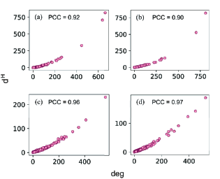
The influence maximization methods we proposed, i.e., HDD and HSD, are degree-based heuristic methods. To check the robustness of our method over the change of the degree heterogeneity [34], we evaluate the performance of our methods on synthetic hypergraphs. Figure 5 indicates that the node degree is positively correlated with the corresponding hyperdegree in the hypergraphs generated by real data, with the Pearson Correlation Coefficient (PCC) higher than 0.5. Therefore, we choose to use HyperCL [35], which is a random hypergraph generator, to generate hypergraph with a certain hyperdegree distribution. The details of HyperCL are given as follows:
Initially, we suppose the hyperdegree and the hyperedge size sequence of a hypergraph are given as and , respectively. For each , the nodes belong to are sampled independently. That is to say, we select node into with probability proportional to its hyperdegree (i.e., the probability is until the size of the hyperedge reaches . Specifically, duplicated nodes are ignored in each hyperedge generation. The algorithm is terminated until the size of each hyperedge reaches the pre-set size.
In the HyperCL, the hyperdegree sequence is generated by a hyperdegree distribution , where the exponent is a tunable parameter. As the value of exponent increases, the hyperdegree distribution would change from heterogeneous to homogeneous. In this work, the exponent value is set as and . The hyperedge size sequence generated by a uniform distribution with the minimum and maximal size setting as and , respectively. We use coefficient of variation (CV), which is defined as the ratio of the standard deviation to the mean, to measure the heterogeneity of the degree distribution of a synthetic hypergraph. In Figure 7, we show that as increases, the CV decreases, indicating that the degree distribution would be more homogeneous. We further show the correlation between the degree and hyperdegree of a node in the synthetic hypergraphs generated by HyperCL in Figure 6, where the PCC is higher than 0.9 in hypergraphs generated by different hyperdegree distribution.
We show the performance of our methods and the baselines on synthetic hypergraphs on influence maximization problem in Figure 7 and Table 7, respectively. We observe that HDD outperforms all the other methods in all the hypergraphs and H-RIS performs the second best. In addition, as decreases, i.e., the degree distribution is more heterogeneous, HDD can gain more improvement in AUC than H-RIS (Table 7). It suggests that HDD tends to be more suitable for solving influence maximization problem in hypergraphs with heterogeneous degree distribution, which is common in real world.


| Hypergraph | AUC | CV | Gain | ||||||
|---|---|---|---|---|---|---|---|---|---|
| HDD | HSD | H-RIS | H-CI() | H-CI() | H-degree | Degree | |||
| 0.1766∗∗ | 0.1540∗ | 0.1510 | 0.1293 | 0.1296 | 0.1293 | 0.1300 | 2.86 | 14.68% | |
| 0.1686∗∗ | 0.1411 | 0.1497∗ | 0.1349 | 0.1349 | 0.1349 | 0.1357 | 2.30 | 12.63% | |
| 0.1581∗∗ | 0.1398 | 0.1476∗ | 0.1387 | 0.1383 | 0.1382 | 0.1394 | 1.49 | 7.11% | |
| 0.1553∗∗ | 0.1405 | 0.1510∗ | 0.1384 | 0.1375 | 0.1384 | 0.1388 | 1.39 | 2.85% | |
5. Conclusions
Much effort has been devoted to find influential node set in ordinary networks. In this work, we tackle the challenge on influence maximization problem in hypergraphs, which aims to identify initial spreaders that can maximize the expected outbreak size of a certain spreading dynamics. We start with a simple spreading model, i.e., susceptible-infected (SI) model with contact process dynamics. Based on the fact that the influence overlap between a node and its neighboring nodes is usually high in hypergraphs generated by real data, we propose an algorithm called Heuristic Degree Discount (HDD) to solve the influence maximization problem in hypergraphs. The algorithm iteratively gives large penalty to nodes that have more neighbors in the existing seed set and thus these nodes are less likely to be chosen as seeds. To validate the effectiveness of our algorithm, we demonstrate a list of baseline algorithms, including the ones proposed by previous researchers as well as algorithms extended from ordinary networks. We perform the experiments on eight hypergraphs generated by real data from various domains. The results show that HDD is superior to the baselines in terms of accuracy (except Greedy) almost in all the hypergraphs with different infection probability. In addition, our algorithm also shows good performance in terms of efficiency. As HDD is based on the node degree, we further test the performance on synthetic hypergraphs generated by HyperCL, which can generate hypergraphs with different hyperdegrees. The results demonstrate HDD gains more AUC scores in hypergraphs with high degree heterogeneity.
Heuristic algorithms have been widely utilized to solve the influence maximization on ordinary networks due to its low computational complexity. In this work, we confine to use a simple heuristic from hypergraph, i.e., degree, to design algorithm for identifying seed node set, which shows high performance. We deem that more high-order properties from hypergraph could be used for influence maximization. Moreover, our algorithm framework could also be promising in solve influence maximization problem for other dynamic processes, such as threshold model [36], independent cascade model [22] and other epidemic models [37, 30].
Acknowledgements
This work was supported by Natural Science Foundation of Zhejiang Province (Grant Nos. LQ22F030008 and LR18A050001), the National Natural Science Foundation of China (Grant Nos. 92146001, 61873080 and 61673151), the Major Project of The National Social Science Fund of China (Grant No. 19ZDA324), and the Scientific Research Foundation for Scholars of HZNU (2021QDL030).
Author Contributions Statement
All authors planed the study. All authors performed the experiments and prepared the figures. All authors analyzed the results and wrote the manuscript. All authors read and approved the final manuscript.
Data and Code Availability
The data and code used in this work can be access via: https://github.com/DDMXIE/Influence-maximization-on-hypergraphs.
References
- [1] C.-H. Cheng, Y.-H. Kuo, Z. Zhou, Outbreak minimization vs influence maximization: an optimization framework, BMC Medical Informatics and Decision Making 20 (1) (2020) 1–13.
- [2] H. Zhang, S. Mishra, M. T. Thai, J. Wu, Y. Wang, Recent advances in information diffusion and influence maximization in complex social networks, Opportunistic Mobile Social Networks 37 (1.1) (2014) 37.
- [3] S. Lei, S. Maniu, L. Mo, R. Cheng, P. Senellart, Online influence maximization, in: Proceedings of the 21th ACM SIGKDD International Conference on Knowledge Discovery and Data Mining, 2015, pp. 645–654.
- [4] P. Domingos, M. Richardson, Mining the network value of customers, in: Proceedings of the seventh ACM SIGKDD International Conference on Knowledge Discovery and Data Mining, 2001, pp. 57–66.
- [5] W. Chen, C. Wang, Y. Wang, Scalable influence maximization for prevalent viral marketing in large-scale social networks, in: Proceedings of the 16th ACM SIGKDD International Conference on Knowledge Discovery and Data Mining, 2010, pp. 1029–1038.
- [6] D. Kempe, J. Kleinberg, É. Tardos, Maximizing the spread of influence through a social network, in: Proceedings of the ninth ACM SIGKDD International Conference on Knowledge Discovery and Data Mining, 2003, pp. 137–146.
- [7] J. Leskovec, A. Krause, C. Guestrin, C. Faloutsos, J. VanBriesen, N. Glance, Cost-effective outbreak detection in networks, in: Proceedings of the 13th ACM SIGKDD International Conference on Knowledge Discovery and Data Mining, 2007, pp. 420–429.
- [8] A. Goyal, W. Lu, L. V. Lakshmanan, Celf++ optimizing the greedy algorithm for influence maximization in social networks, in: Proceedings of the 20th International Conference Companion on World Wide Web, 2011, pp. 47–48.
- [9] A. Goyal, W. Lu, L. V. Lakshmanan, Simpath: An efficient algorithm for influence maximization under the linear threshold model, in: 2011 IEEE 11th International Conference on Data Mining, IEEE, 2011, pp. 211–220.
- [10] Y.-C. Chen, W.-Y. Zhu, W.-C. Peng, W.-C. Lee, S.-Y. Lee, Cim: community-based influence maximization in social networks, ACM Transactions on Intelligent Systems and Technology (TIST) 5 (2) (2014) 1–31.
- [11] H. T. Nguyen, M. T. Thai, T. N. Dinh, Stop-and-stare: Optimal sampling algorithms for viral marketing in billion-scale networks, in: Proceedings of the 2016 International Conference on Management of Data, 2016, pp. 695–710.
- [12] R. Narayanam, Y. Narahari, A shapley value-based approach to discover influential nodes in social networks, IEEE Transactions on Automation Science and Engineering 8 (1) (2010) 130–147.
- [13] C. Wang, W. Chen, Y. Wang, Scalable influence maximization for independent cascade model in large-scale social networks, Data Mining and Knowledge Discovery 25 (3) (2012) 545–576.
- [14] Y. Tang, X. Xiao, Y. Shi, Influence maximization: Near-optimal time complexity meets practical efficiency, in: Proceedings of the 2014 ACM SIGMOD International Conference on Management of data, 2014, pp. 75–86.
- [15] G. Cencetti, F. Battiston, B. Lepri, M. Karsai, Temporal properties of higher-order interactions in social networks, Scientific reports 11 (1) (2021) 1–10.
- [16] J.-G. Young, G. Petri, T. P. Peixoto, Hypergraph reconstruction from network data, Communications Physics 4 (1) (2021) 1–11.
- [17] M. Kitsak, I. Voitalov, D. Krioukov, Link prediction with hyperbolic geometry, Physical Review Research 2 (4) (2020) 043113.
- [18] X. Ouvrard, Hypergraphs: an introduction and review, arXiv preprint arXiv:2002.05014 (2020).
- [19] F. Amato, V. Moscato, A. Picariello, G. Sperlí, Influence maximization in social media networks using hypergraphs, in: International Conference on Green, Pervasive, and Cloud Computing, Springer, 2017, pp. 207–221.
- [20] Y. Tang, Y. Shi, X. Xiao, Influence maximization in near-linear time: A martingale approach, in: Proceedings of the 2015 ACM SIGMOD International Conference on Management of Data, 2015, pp. 1539–1554.
- [21] J. Zhu, J. Zhu, S. Ghosh, W. Wu, J. Yuan, Social influence maximization in hypergraph in social networks, IEEE Transactions on Network Science and Engineering 6 (4) (2018) 801–811.
- [22] A. MA, A. Rajkumar, Hyper-imrank: Ranking-based influence maximization for hypergraphs, in: 5th Joint International Conference on Data Science & Management of Data (9th ACM IKDD CODS and 27th COMAD), 2022, pp. 100–104.
- [23] A. Antelmi, G. Cordasco, C. Spagnuolo, P. Szufel, Social influence maximization in hypergraphs, Entropy 23 (7) (2021) 796.
- [24] L. Lü, D. Chen, X.-L. Ren, Q.-M. Zhang, Y.-C. Zhang, T. Zhou, Vital nodes identification in complex networks, Physics Reports 650 (2016) 1–63.
- [25] C. Stegehuis, T. Peron, Network processes on clique-networks with high average degree: the limited effect of higher-order structure, Journal of Physics: Complexity 2 (4) (2021) 045011.
- [26] Q. Suo, J.-L. Guo, A.-Z. Shen, Information spreading dynamics in hypernetworks, Physica A: Statistical Mechanics and its Applications 495 (2018) 475–487.
- [27] F. Battiston, G. Cencetti, I. Iacopini, V. Latora, M. Lucas, A. Patania, J.-G. Young, G. Petri, Networks beyond pairwise interactions: structure and dynamics, Physics Reports 874 (2020) 1–92.
- [28] Y. Li, J. Fan, Y. Wang, K.-L. Tan, Influence maximization on social graphs: A survey, IEEE Transactions on Knowledge and Data Engineering 30 (10) (2018) 1852–1872.
- [29] G. Ferraz de Arruda, M. Tizzani, Y. Moreno, Phase transitions and stability of dynamical processes on hypergraphs, Communications Physics 4 (1) (2021) 1–9.
- [30] G. F. de Arruda, G. Petri, Y. Moreno, Social contagion models on hypergraphs, Physical Review Research 2 (2) (2020) 023032.
- [31] X.-X. Zhan, Z. Li, N. Masuda, P. Holme, H. Wang, Susceptible-infected-spreading-based network embedding in static and temporal networks, EPJ Data Science 9 (1) (2020) 30.
- [32] C. Borgs, M. Brautbar, J. Chayes, B. Lucier, Maximizing social influence in nearly optimal time, in: Proceedings of the 25th annual ACM-SIAM symposium on Discrete algorithms, SIAM, 2014, pp. 946–957.
- [33] F. Morone, H. A. Makse, Influence maximization in complex networks through optimal percolation, Nature 524 (7563) (2015) 65–68.
- [34] G. St-Onge, I. Iacopini, V. Latora, A. Barrat, G. Petri, A. Allard, L. Hébert-Dufresne, Influential groups for seeding and sustaining nonlinear contagion in heterogeneous hypergraphs, Communications Physics 5 (1) (2022) 1–16.
- [35] G. Lee, M. Choe, K. Shin, How do hyperedges overlap in real-world hypergraphs?-patterns, measures, and generators, in: Proceedings of the Web Conference 2021, 2021, pp. 3396–3407.
- [36] X.-J. Xu, S. He, L.-J. Zhang, Dynamics of the threshold model on hypergraphs, Chaos: An Interdisciplinary Journal of Nonlinear Science 32 (2) (2022) 023125.
- [37] B. Jhun, M. Jo, B. Kahng, Simplicial SIS model in scale-free uniform hypergraph, Journal of Statistical Mechanics: Theory and Experiment 2019 (12) (2019) 123207.