Inference in parametric models with many L-moments

As in the previous section, we consider a setting where we have a sample with $T$ identically distributed observations, $Y_{1},Y_{2}\ldots Y_{T}$, $Y_{t}\sim F$ for $t=1,2\ldots T$, where $F$ belongs to a parametric family $\{F_{\theta}:\theta\in\Theta\}$, $\Theta\subseteq\mathbb{R}^{d}$; and $F=F_{\theta_{0}}$ for some $\theta_{0}\in\Theta$. We will analyse the behaviour of the estimator:

where $\hat{Q}_{Y}(\cdot)$ is the empirical quantile process given by (4); $Q_{Y}(\cdot|\theta)$ is the quantile function associated with $F_{\theta}$; $\{w_{k,l}^{R}\}_{1\leq k,l\leq R}$ are a set of (possibly estimated) weights; $\{P_{k}\}_{1\leq k\leq R}$ are a set of quantile “weighting” functions with $\int_{0}^{1}P_{k}(u)^{2}du=1$; and $0\leq\underline{p}<\bar{p}\leq 1$. This setting encompasses the generalised-method-of-L-moment estimatior discussed in the previous section. Indeed, by choosing $P_{k}(u)=\sqrt{2(2k-1)}\cdot P^{*}_{k-1}(u)$, where $P^{*}_{k}(u)$ are the shifted Legendre polynomials on $[0,1]$, and $0=\underline{p}<\bar{p}=1$, we have the generalised L-moment-based estimator in (6) using (3) as an estimator for the L-moments.⁷⁷7The rescaling by $\sqrt{2(2k-1)}$ is adopted so the polynomials have unit $L^{2}[0,1]$-norm. We leave $\underline{p}<\bar{p}$ fixed throughout.⁸⁸8In Remark 4 later on, we briefly discuss an extension to sample-size-dependent trimming. All limits are taken jointly with respect to $T$ and $R$.

To facilitate analysis, we let $\mathbf{P}^{R}(u)\coloneqq(P_{1}(u),P_{2}(u)\ldots P_{R}(u))^{\prime}$; and write $W^{R}$ for the $R\times R$ matrix with entry $W_{i,j}^{R}=w_{i,j}^{R}$. We may then rewrite our estimator in matrix form as:

In this section, we present conditions under which our estimator is consistent.

We impose the following assumptions on our environment. In what follows, we write $Q_{Y}(\cdot)=Q_{Y}(\cdot|\theta_{0})$.

1 is satisfied in a variety of settings. For example, if $Y_{1}$, $Y_{2}$ …$Y_{T}$ are iid and the family $\{F_{\theta}:\theta\in\Theta\}$ is continuous with a (common) compact support; then (8) follows with $\underline{p}=0$ and $\overline{p}=1$ (Ahidar-Coutrix and Berthet, 2016, Proposition 2.1.). Yoshihara (1995) and Portnoy (1991) provide sufficient conditions for uniform consistency (8) to hold when observations are dependent. We also note that, for the result in this section, it would have been sufficient to assume weak convergence in the $L^{2}(\underline{p},\bar{p})$ norm (see Mason (1984), Barrio et al. (2005) and references therein). We only state results in the $\sup$-norm because convergence statements regarding the empirical quantile process available in the literature are usually proved in $L^{\infty}(\underline{p},\bar{p})$.

2 is satisfied by (rescaled) shifted Legendre polynomials, shifted Jacobi polynomials and other weighting functions.

Next, we impose restrictions on the estimated weights. In what follows, we write, for a $c\times d$ matrix $A$, $\lVert A\rVert_{2}=\sqrt{\lambda_{\max}(A^{\prime}A)}$.

3 restricts the range of admissible weight matrices. Notice that $W^{R}=\Omega^{R}=\mathbb{I}_{R}$ trivially satisfies these assumptions. By the triangle inequality, 3 implies that $\lVert W^{R}\rVert_{2}=O_{P^{*}}(1)$.

Finally, we introduce our identifiability assumption. For some $X\in L^{2}[0,1]$, let $\lVert X\rVert_{L^{2}[0,1]}=\left(\int_{0}^{1}X(u)^{2}du\right)^{\frac{1}{2}}$:

The first part of this assumption is closely related to the usual notion of identifiability in parametric distribution models. Indeed, if $\Theta$ is compact, $\theta\mapsto\lVert Q(\cdot|\theta)\rVert_{L^{2}[0,1]}$ is continuous, $\underline{p}=0$, $\bar{p}=1$, the $\{P_{l}\}_{l}$ constitute an orthonormal basis in $L^{2}[0,1]$ (this is the case for shifted Legendre polynomials), and $W^{R}=\mathbb{I}_{R}$, then part 1 is equivalent to identifiability of the parametric family $\{F_{\theta}\}_{\theta}$.

As for the second part of the assumption, we note that boundedness of the $L^{2}$ norm of parametric quantiles uniformly in $\theta$ is satisfied in several settings. If the parametric family $\{F_{\theta}:\theta\in\Theta\}$ has common compact support, then the assumption is trivially satisfied. More generally, if we assume $\Theta$ is compact and $Q_{Y}(u|\theta)$ is jointly continuous and bounded on $[\underline{p},\bar{p}]\times\Theta$, then the condition follows immediately from Weierstrass’ theorem, as in this case: $\sup_{\theta\in\Theta}\lVert Q_{Y}(\cdot|\theta)\mathbbm{1}_{[\underline{p},\bar{p}]}\rVert_{L^{2}[0,1]}\leq\sqrt{\bar{p}-\underline{p}}\cdot\sup_{(\theta,u)\in\Theta\times[\underline{p},\bar{p}]}|Q_{Y}(u|\theta)|<\infty$.

Under the previous assumptions, the estimator is consistent.

In this section, we provide conditions under which the estimator admits an asymptotic linear representation. In what, follows, define $h^{R}(\theta):=\int_{\underline{p}}^{\bar{p}}\left(\hat{Q}_{Y}(u)-Q_{Y}(u|\theta)\right)\mathbf{P}^{R}(u)du$; and write $\nabla_{\theta^{\prime}}h^{R}(\tilde{\theta})$ for the Jacobian of $h^{R}$ with respect to $\theta$, evaluated at $\tilde{\theta}$. We assume that:

Assumption 5 requires $\theta_{0}$ to be an interior point of $\Theta$. It also implies the objective function is countinuously differentiable on a neighborhood of $\theta_{0}$, which enables us to linearise the first order condition satisfied with high probability by $\hat{\theta}$.

Weak convergence of the empirical quantile process (6) has been derived in a variety of settings, ranging from iid data (Vaart, 1998, Corollary 21.5) to nonstationary and weakly dependent observations (Portnoy, 1991). In the iid setting, if the family $\{F_{\theta}:\theta\in\Theta\}$ is continuously differentiable with strictly positive density $f_{\theta}$ over a (common) compact support; then weak-convergence holds with $\underline{p}=0$ and $\overline{p}=1$. In this case, the covariance kernel is $\Gamma(i,j)=\frac{(i\land j-ij)}{f_{Y}(Q_{Y}(i))f_{Y}(Q_{Y}(j))}$. Similarly to the discussion of Assumption 1, Assumption 6 is stronger than necessary: it would have been sufficient to assume $\lVert\sqrt{T}(Q_{Y}(\cdot)-\hat{Q}_{Y}(\cdot))\mathbbm{1}_{[\underline{p},\bar{p}]}\rVert_{L^{2}[0,1]}^{2}=O_{P^{*}}(1)$, which is implied by weak convergence in $L^{2}$.

7 is a technical condition which enables us to provide an upper bound to the linearisation error of the first order condition satisfied by $\hat{\theta}$.

8 is similar to the rank condition used in the proof of asymptotic normality of M-estimators (Newey and McFadden, 1994), which is known to be equivalent to a local identification condition under rank-regularity assumptions (Rothenberg, 1971). In our setting, where $R$ varies with sample size, we show in Supplemental LABEL:app_relation that a stronger version of 4 implies 8.

Under Assumptions 1-8, we have that:

In the next subsection, we work out an asymptotic approximation to the distribution of the leading term in (9).

Finally, to work out the asymptotic distribution of the proposed estimator, we rely on a strong approximation concept. The idea is to construct, in the same underlying probability space, a sequence of Brownian bridges that approximates, in the supremum norm, the empirical quantile process. This can then be used to conduct inference based on a Gaussian distribution. In Supplemental Appendix LABEL:app_inferece_bahadur, we alternatively show how a Bahadur-Kiefer representation of the quantile process can be used to conduct inference in the iid case. In this alternative, one approximates the distribution of the leading term of (9) by a transformation of independent Bernoulli random variables.

We first consider a strong approximation to a Gaussian process in the iid setting. We state below a classical result, due to Csorgo and Revesz (1978):

The above theorem is much stronger than the weak convergence of 6. Indeed, Theorem 1 requires variables to be defined in the same probability space and yields explicit bounds in the sup norm; whereas weak convergence is solely a statement on the convergence of integrals (Vaart and Wellner, 1996). Suppose the approximation (10)/(11) holds in our context. Let $B_{T}$ be as in the statement of the theorem, and assume in addition that $\int_{\underline{p}}^{\overline{p}}\frac{1}{f_{Y}(Q_{Y}(u))^{2}}du<\infty$. A simple application of Bessel’s inequality then shows that:

Note that the distribution of the leading term in the right-hand side is known (by Riemann integration, it is Gaussian) up to $\theta_{0}$. This representation could thus be used as a basis for inference. The validity of such approach can be justified by verifying that the Kolmogorov distance between the distribution of $\sqrt{T}(\hat{\theta}-\theta_{0})$ and that of the leading term of the representation goes to zero as $T$ and $R$ increase. We show that this indeed is true later on, where convergence in the Kolmogorov distance is obtained as a byproduct of weak convergence.

Next, we reproduce a strong approximation result in the context of dependent observations. The result is due to Fotopoulos and Ahn (1994) and Yu (1996).

A similar argument as the previous one then shows that, under the conditions of the theorem above:

Differently from the iid case, the distribution of the leading term on the right-hand side is now known up to $\theta_{0}$ and the covariance kernel $\Gamma$. The latter could be estimated with a Newey and West (1987) style estimator.

To conclude the discussion, we note that the strong representation (12) (resp. (14)) allows us to establish asymptotic normality of our estimator. Indeed, let $L_{T}$ be the leading term of the representation on the right-hand side of (12) (resp. (14)), and $V_{T,R}$ be its variance. Observe that ${V}_{T,R}^{-1/2}R_{T}$ is distributed according to a multivariate standard normal. It then follows by Slutsky’s theorem that $V_{T,R}^{-1/2}\sqrt{T}(\hat{\theta}-\theta_{0})\overset{d}{\to}N(0,\mathbb{I}_{d})$. Since pointwise convergence of cdfs to a continuous cdf implies uniform convergence (Parzen, 1960, page 438), and given that $V_{T,R}^{-1/2}$ is positive definite, we obtain that:

which justifies our approach to inference based on the distribution of the leading term on the right-hand side of (12) (resp. (14)).

We collect the main results in this subsection under the corollary below.

Supplemental Appendix LABEL:app_efficiency discusses efficiency of our proposed L-moment estimator. Specifically, we show that, when no trimming is adopted ($0=\underline{p}<\overline{p}=1$), the optimal weighting scheme (16) is used, the $\{P_{l}\}_{l}$ constitue an orthonormal basis in $L^{2}[0,1]$ (recall this is satisfied by shifted Legendre polynomials), and the data is iid, the generalised method of L-moments estimator is assymptotically efficient, in the sense that its asymptotic variance coincides with the inverse of the Fisher information matrix of the parametric model.¹⁰¹⁰10In the dependent case, “efficiency” should be defined as achieving the efficiency bound of the semiparametric model that parametrises the marginal distribution of the $Y_{t}$, but leaves the time series dependence unrestricted up to regularity conditions (Newey, 1990; Komunjer and Vuong, 2010). Indeed, in general, our L-moment estimator will be inefficient with respect to the MLE estimator that models the dependency structure between observations. See Carrasco and Florens (2014) for further discussion. We leave details to the Supplemental Appendix, though we briefly outline the argument here. The idea is to consider the alternative estimator:

for a grid of $G_{T}$ points $\mathcal{G}_{T}=\{g_{1},g_{2},\ldots,g_{G_{T}}\}\subseteq(0,1)$ and weights $\kappa_{i,j}$, $i,j\in\mathcal{G}_{T}$. This is a weighted version of a “percentile-based estimator”, which is used in contexts where it is difficult to maximise the likelihood (Gupta and Kundu, 2001). It amounts to choosing $\theta$ so as to match a weighted combination of the order statistics in the sample. In the Supplemental Appendix, we show that, under a suitable sequence of gridpoints and optimal weights, this estimator is asympotically efficient. We then show, by using the fact that the $\{P_{l}\}_{l}$ form an orthonormal basis, that estimator (17) can be seen as a generalised L-moment estimator that uses infinitely many L-moments. The final step of the argument then consists in showing that a generalised L-moment estimator that uses a finite but increasing number of L-moments is asymptotically equivalent to estimator (17), which implies that a generalised L-moment estimator under optimal weights is no less efficient than the (efficient) percentile estimator.

Following Hosking et al. (1985) and Hosking (1990), we consider the family of distributions

and $\theta_{0}=(0,1,-0.2)^{\prime}$.

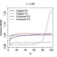
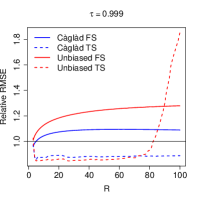
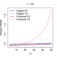
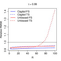
Table 1 reports the RMSE of each procedure, divided by the RMSE of the MLE, under the choice of $R$ that achieves the smallest RMSE. Values above 1 indicate the MLE outperforms the estimator in consideration; and values below 1 indicate the estimator outperforms MLE. The value of $R$ that minimises the RMSE is presented under parentheses. Some patterns are worth highlighting. Firstly, the L-moment estimator, under a proper choice of $R$ and (estimated) optimal weights (two-step estimators) is able to outperform MLE in most settings, especially at the tail of the distribution function. Reductions in these settings can be as large as $34\%$. At the median, two-step L-moment estimators behave similarly to the MLE. The performance of two-step càglàd and unbiased estimators is also quite similar. Secondly, the power of overidentifying restrictions is evident: except in four out of twenty-four cases, two-step L-moment estimators never achieve a minimum RMSE at $R=3$, the number of parameters. These exceptions are found at the smallest sample size ($T=50$), where the benefit of overidentifying restrictions may be outweighed by noisy estimation of the weighting matrix.¹³¹³13Indeed, as we discuss in Supplemental Appendix LABEL:app_selection, a higher-order expansion of our proposed estimator shows that correlation of the estimator of the optimal weighting matrix with sample L-moments plays a key role in the higher-order bias and variance of the two-step estimator. Thirdly, the relation between $T$ and $R$ in the two-step Càglàd estimator is monotonic, as expected from our theoretical discussion. Finally, the role of optimal weights is clear: first-step estimators tend to underperform the MLE as the sample size increases. In larger samples, and when optimal weights are not used, the best choice tends to be setting $R$ close to or equal to $3$, which reinforces the importance of weighting when overidentifying restrictions are included.

To better understand the patterns in the table, we report in Figure 1, the relative RMSE curve for different sample sizes and choices of $R$. The role of optimal weights is especially striking: first-step estimators usually exhibit an increasing RMSE, as a function of $R$. In contrast, two-step estimators are able to better control the RMSE across $R$. It is also interesting to note that the two-step unbiased L-moment estimator behaves poorly when $R$ is close to $T$. This suggests that, in settings where one may wish to make $R$ large, the càglád estimator is preferrable.¹⁴¹⁴14This is also in accordance with our theoretical results for the càglád-based estimator, which essentially place no restriction on the growth rate of $R$.

Following Hosking and Wallis (1987), we consider the family of distributions:

and $\theta_{0}=(1,-0.2)^{\prime}$.

Table 2 and Figure 2 summarise the results of our simulation. Overall patterns are similar to the ones obtained in the GEV simulations. Importantly, though, estimation of the optimal weighting matrix impacts two-step estimators quite negatively in this setup. As a consequence, we verify that the choice of $R=2$ (i.e. a just-identified estimator that effectively does not rely on the weights) is optimal for TS estimators at eight out of the sixteen cases in sample sizes smaller than $500$. This behaviour also leads to FS estimators, which do not use estimated weights, outperforming TS estimators at the $0.99$ and $0.999$ quantiles when $T=50$, and only slightly underperforming TS estimators at some quantiles in larger sample sizes. The latter phenomenon is also partly explained by the just-identified choice $R=2$ improving upon the MLE even in the largest sample size. In all settings, L-moment estimators compare favourably to the MLE.

References

- Abadie et al. (2023) Abadie, A., J. Gu, and S. Shen (2023). Instrumental variable estimation with first-stage heterogeneity. Journal of Econometrics.
- Ahidar-Coutrix and Berthet (2016) Ahidar-Coutrix, A. and P. Berthet (2016). Convergence of multivariate quantile surfaces. arXiv:1607.02604.
- Ai and Chen (2003) Ai, C. and X. Chen (2003). Efficient estimation of models with conditional moment restrictions containing unknown functions. Econometrica 71(6), 1795–1843.
- Alvarez and Biderman (2024) Alvarez, L. and C. Biderman (2024). The learning effects of subsidies to bundled goods: a semiparametric approach.
- Alvarez and Orestes (2023) Alvarez, L. and V. Orestes (2023). Quantile mixture models: Estimation and inference. Technical report.
- Anderson and Hsiao (1982) Anderson, T. and C. Hsiao (1982). Formulation and estimation of dynamic models using panel data. Journal of Econometrics 18(1), 47–82.
- Arellano and Bond (1991) Arellano, M. and S. Bond (1991, 04). Some Tests of Specification for Panel Data: Monte Carlo Evidence and an Application to Employment Equations. The Review of Economic Studies 58(2), 277–297.
- Athey et al. (2023) Athey, S., P. J. Bickel, A. Chen, G. W. Imbens, and M. Pollmann (2023, 07). Semi-parametric estimation of treatment effects in randomised experiments. Journal of the Royal Statistical Society Series B: Statistical Methodology 85(5), 1615–1638.
- Athey et al. (2019) Athey, S., J. Tibshirani, and S. Wager (2019). Generalized random forests. The Annals of Statistics 47(2), 1148 – 1178.
- Barrio et al. (2005) Barrio, E. D., E. Giné, and F. Utzet (2005). Asymptotics for L2 functionals of the empirical quantile process, with applications to tests of fit based on weighted Wasserstein distances. Bernoulli 11(1), 131 – 189.
- Belloni et al. (2012) Belloni, A., D. Chen, V. Chernozhukov, and C. Hansen (2012). Sparse models and methods for optimal instruments with an application to eminent domain. Econometrica 80(6), 2369–2429.
- Belloni et al. (2019) Belloni, A., V. Chernozhukov, D. Chetverikov, and I. Fernández-Val (2019). Conditional quantile processes based on series or many regressors. Journal of Econometrics 213(1), 4 – 29. Annals: In Honor of Roger Koenker.
- Biderman (2018) Biderman, C. (2018, October). E-hailing and last mile connectivity in sao paulo. American Economic Association Registry for Randomized Controlled Trials. AEARCTR-0003518.
- Billingsley (2012) Billingsley, P. (2012). Probability and Measure. Wiley.
- Boulange et al. (2021) Boulange, J., N. Hanasaki, D. Yamazaki, and Y. Pokhrel (2021). Role of dams in reducing global flood exposure under climate change. Nature communications 12(1), 1–7.
- Broniatowski and Decurninge (2016) Broniatowski, M. and A. Decurninge (2016). Estimation for models defined by conditions on their L-moments. IEEE Transactions on Information Theory 62(9), 5181–5198.
- Carrasco and Florens (2014) Carrasco, M. and J.-P. Florens (2014). On the asymptotic efficiency of gmm. Econometric Theory 30(2), 372–406.
- Castellacci (2012) Castellacci, G. (2012). A formula for the quantiles of mixtures of distributions with disjoint supports. Available at SSRN 2055022.
- Chernozhukov et al. (2018) Chernozhukov, V., D. Chetverikov, M. Demirer, E. Duflo, C. Hansen, W. Newey, and J. Robins (2018, 01). Double/debiased machine learning for treatment and structural parameters. The Econometrics Journal 21(1), C1–C68.
- Chernozhukov et al. (2022) Chernozhukov, V., J. C. Escanciano, H. Ichimura, W. K. Newey, and J. M. Robins (2022). Locally robust semiparametric estimation. Econometrica 90(4), 1501–1535.
- Chernozhukov and Fernández-Val (2011) Chernozhukov, V. and I. Fernández-Val (2011). Inference for extremal conditional quantile models, with an application to market and birthweight risks. The Review of Economic Studies 78(2), 559–589.
- Crump et al. (2009) Crump, R. K., V. J. Hotz, G. W. Imbens, and O. A. Mitnik (2009, 01). Dealing with limited overlap in estimation of average treatment effects. Biometrika 96(1), 187–199.
- Csorgo and Revesz (1978) Csorgo, M. and P. Revesz (1978, 07). Strong approximations of the quantile process. Annals of Statistics 6(4), 882–894.
- Das (2021) Das, S. (2021). Extreme rainfall estimation at ungauged locations: information that needs to be included in low-lying monsoon climate regions like bangladesh. Journal of Hydrology 601, 126616.
- Dey et al. (2018) Dey, S., J. Mazucheli, and S. Nadarajah (2018, may). Kumaraswamy distribution: different methods of estimation. Computational and Applied Mathematics 37(2), 2094–2111.
- Donald et al. (2003) Donald, S. G., G. W. Imbens, and W. K. Newey (2003). Empirical likelihood estimation and consistent tests with conditional moment restrictions. Journal of Econometrics 117(1), 55–93.
- Donald et al. (2009) Donald, S. G., G. W. Imbens, and W. K. Newey (2009). Choosing instrumental variables in conditional moment restriction models. Journal of Econometrics 152(1), 28–36.
- Donald and Newey (2001) Donald, S. G. and W. K. Newey (2001). Choosing the number of instruments. Econometrica 69(5), 1161–1191.
- Ferrari and Yang (2010) Ferrari, D. and Y. Yang (2010, 04). Maximum l q -likelihood estimation. Annals of Statistics 38(2), 753–783.
- Foss et al. (2011) Foss, S., D. Korshunov, S. Zachary, et al. (2011). An introduction to heavy-tailed and subexponential distributions, Volume 6. Springer.
- Fotopoulos and Ahn (1994) Fotopoulos, S. and S. Ahn (1994). Strong approximation of the quantile processes and its applications under strong mixing properties. Journal of Multivariate Analysis 51(1), 17–45.
- Freyberger and Rai (2018) Freyberger, J. and Y. Rai (2018). Uniform confidence bands: Characterization and optimality. Journal of Econometrics 204(1), 119–130.
- Götze et al. (2019) Götze, F., A. Naumov, V. Spokoiny, and V. Ulyanov (2019). Large ball probabilities, Gaussian comparison and anti-concentration. Bernoulli 25(4A), 2538 – 2563.
- Gourieroux and Jasiak (2008) Gourieroux, C. and J. Jasiak (2008). Dynamic quantile models. Journal of Econometrics 147(1), 198–205.
- Guerre and Sabbah (2012) Guerre, E. and C. Sabbah (2012). Uniform bias study and bahadur representation for local polynomial estimators of the conditional quantile function. Econometric Theory 28(1), 87–129.
- Gupta and Kundu (2001) Gupta, R. D. and D. Kundu (2001). Generalized exponential distribution: Different method of estimations. Journal of Statistical Computation and Simulation 69(4), 315–337.
- Hahn et al. (2002) Hahn, J., G. Kuersteiner, and W. Newey (2002). Higher order properties of bootstrap and jackknife bias corrected maximum likelihood estimators. Unpublished manuscript.
- Han and Phillips (2006) Han, C. and P. C. B. Phillips (2006). Gmm with many moment conditions. Econometrica 74(1), 147–192.
- Hansen (1982) Hansen, L. P. (1982). Large sample properties of generalized method of moments estimators. Econometrica 50(4), 1029–1054.
- Hosking (1986) Hosking, J. R. (1986). The theory of probability weighted moments. IBM Research Division, TJ Watson Research Center New York, USA.
- Hosking (2007) Hosking, J. R. (2007). Some theory and practical uses of trimmed L-moments. Journal of Statistical Planning and Inference 137(9), 3024–3039.
- Hosking (1990) Hosking, J. R. M. (1990, sep). L-Moments: Analysis and Estimation of Distributions Using Linear Combinations of Order Statistics. Journal of the Royal Statistical Society: Series B (Methodological) 52(1), 105–124.
- Hosking and Wallis (1987) Hosking, J. R. M. and J. R. Wallis (1987). Parameter and quantile estimation for the generalized pareto distribution. Technometrics 29(3), 339–349.
- Hosking et al. (1985) Hosking, J. R. M., J. R. Wallis, and E. F. Wood (1985). Estimation of the generalized extreme-value distribution by the method of probability-weighted moments. Technometrics 27(3), 251–261.
- Ichimura and Newey (2022) Ichimura, H. and W. K. Newey (2022). The influence function of semiparametric estimators. Quantitative Economics 13(1), 29–61.
- Kennedy (2023) Kennedy, E. H. (2023). Semiparametric doubly robust targeted double machine learning: a review.
- Kerstens et al. (2011) Kerstens, K., A. Mounir, and I. V. De Woestyne (2011). Non-parametric frontier estimates of mutual fund performance using C- and L-moments: Some specification tests. Journal of Banking and Finance 35(5), 1190–1201.
- Koenker and Machado (1999) Koenker, R. and J. A. Machado (1999). Gmm inference when the number of moment conditions is large. Journal of Econometrics 93(2), 327–344.
- Komunjer and Vuong (2010) Komunjer, I. and Q. Vuong (2010). Semiparametric efficiency bound in time-series models for conditional quantiles. Econometric Theory 26(2), 383–405.
- Kreyszig (1989) Kreyszig, E. (1989). Introductory Functional Analysis with Applications. Wiley.
- Landwehr et al. (1979) Landwehr, J. M., N. C. Matalas, and J. R. Wallis (1979). Probability weighted moments compared with some traditional techniques in estimating gumbel parameters and quantiles. Water Resources Research 15(5), 1055–1064.
- Li et al. (2021) Li, C., F. Zwiers, X. Zhang, G. Li, Y. Sun, and M. Wehner (2021). Changes in annual extremes of daily temperature and precipitation in cmip6 models. Journal of Climate 34(9), 3441–3460.
- Luo et al. (2015) Luo, Y. et al. (2015). High-dimensional econometrics and model selection. Ph. D. thesis, Massachusetts Institute of Technology.
- Mason (1984) Mason, D. M. (1984, 02). Weak convergence of the weighted empirical quantile process in . Annals of Probability 12(1), 243–255.
- Meinshausen (2006) Meinshausen, N. (2006). Quantile regression forests. Journal of Machine Learning Research 7(35), 983–999.
- Newey (1990) Newey, W. K. (1990). Semiparametric efficiency bounds. Journal of Applied Econometrics 5(2), 99–135.
- Newey and McFadden (1994) Newey, W. K. and D. McFadden (1994). Chapter 36 large sample estimation and hypothesis testing. In Handbook of Econometrics, Volume 4, pp. 2111 – 2245. Elsevier.
- Newey and Smith (2004) Newey, W. K. and R. J. Smith (2004). Higher order properties of gmm and generalized empirical likelihood estimators. Econometrica 72(1), 219–255.
- Newey and West (1987) Newey, W. K. and K. D. West (1987). A simple, positive semi-definite, heteroskedasticity and autocorrelation consistent covariance matrix. Econometrica 55(3), 703–708.
- Okui (2009) Okui, R. (2009). The optimal choice of moments in dynamic panel data models. Journal of Econometrics 151(1), 1–16.
- Parzen (1960) Parzen, E. (1960). Modern probability theory and its applications. Wiley.
- Pfanzagl and Wefelmeyer (1978) Pfanzagl, J. and W. Wefelmeyer (1978). A third-order optimum property of the maximum likelihood estimator. Journal of Multivariate Analysis 8(1), 1–29.
- Portnoy (1991) Portnoy, S. (1991). Asymptotic behavior of regression quantiles in non-stationary, dependent cases. Journal of Multivariate Analysis 38(1), 100 – 113.
- Rothenberg (1971) Rothenberg, T. J. (1971). Identification in parametric models. Econometrica 39(3), 577–91.
- Sankarasubramanian and Srinivasan (1999) Sankarasubramanian, A. and K. Srinivasan (1999). Investigation and comparison of sampling properties of L-moments and conventional moments. Journal of Hydrology 218(1-2), 13–34.
- Šimková (2017) Šimková, T. (2017). Statistical inference based on L-moments. Statistika 97(1), 44–58.
- Vaart (1998) Vaart, A. W. v. d. (1998). Asymptotic Statistics. Cambridge Series in Statistical and Probabilistic Mathematics. Cambridge University Press.
- Vaart and Wellner (1996) Vaart, A. W. V. d. and J. A. Wellner (1996). Weak convergence and empirical processes. Springer.
- Wang and Hutson (2013) Wang, D. and A. D. Hutson (2013). Joint confidence region estimation of L-moment ratios with an extension to right censored data. Journal of Applied Statistics 40(2), 368–379.
- Wang (1997) Wang, Q. J. (1997). LH moments for statistical analysis of extreme events. Water Resources Research 33(12), 2841–2848.
- Wooldridge (2010) Wooldridge, J. (2010). Econometric analysis of cross section and panel data. Cambridge, Mass: MIT Press.
- Yang et al. (2021) Yang, J., Z. Bian, J. Liu, B. Jiang, W. Lu, X. Gao, and H. Song (2021). No-reference quality assessment for screen content images using visual edge model and adaboosting neural network. IEEE Transactions on Image Processing 30, 6801–6814.
- Yoshihara (1995) Yoshihara, K. (1995). The bahadur representation of sample quantiles for sequences of strongly mixing random variables. Statistics & Probability Letters 24(4), 299 – 304.
- Yu (1996) Yu, H. (1996). A note on strong approximation for quantile processes of strong mixing sequences. Statistics & Probability Letters 30(1), 1 – 7.
- Yu and Jones (1998) Yu, K. and M. C. Jones (1998). Local linear quantile regression. Journal of the American Statistical Association 93(441), 228–237.
See pages - of supplemental.pdf