Inertial range statistics of the Entropic Lattice Boltzmann in 3D turbulence
Abstract
We present a quantitative analysis of the inertial range statistics produced by Entropic Lattice Boltzmann Method (ELBM) in the context of 3d homogeneous and isotropic turbulence. ELBM is a promising mesoscopic model particularly interesting for the study of fully developed turbulent flows because of its intrinsic scalability and its unconditional stability. In the hydrodynamic limit, the ELBM is equivalent to the Navier-Stokes equations with an extra eddy viscosity term Malaspinas2008 . From this macroscopic formulation, we have derived a new hydrodynamical model that can be implemented as a Large-Eddy Simulation (LES) closure. This model is not positive definite, hence, able to reproduce backscatter events of energy transferred from the subgrid to the resolved scales. A statistical comparison of both mesoscopic and macroscopic entropic models based on the ELBM approach is presented and validated against fully resolved Direct Numerical Simulations (DNS). Besides, we provide a second comparison of the ELBM with respect to the well known Smagorinsky closure. We found that ELBM is able to extend the energy spectrum scaling range preserving at the same time the simulation stability. Concerning the statistics of higher order, inertial range observables, ELBM accuracy is shown to be comparable with other approaches such as Smagorinsky model.
I Introduction
Turbulence is common in nature and its unpredictable behavior has fundamental consequences on the understanding and control of various systems, from smaller engineering devices dumitrescu2004rotational ; Davidson2015 ; Pope2001 , up to the larger scales geophysical and astrophysical flows gill2016atm ; alexakis2018 ; barnes2001 . Turbulent flows are described by the Navier-Stokes equations (NSE),
| (1) |
which give the evolution of the incompressible velocity field , with kinematic viscosity , subject to a pressure field and to an external forcing . However, even though the equations of motion are known since almost two hundred years a direct analytical approach remains elusive Frisch1995 . To overcome mathematical difficulties, scientists, helped by the exponential growth of the computational power, have tried to search for approximate solutions using numerical algorithms fox2003computational ; Pope2001 ; ishihara2009study . Unfortunately, also in this direction not every effort were successful. Indeed, the NSE have a very rich non-linear dynamics, where a large range of scales from the domain size up to the small scales fluctuations, are coupled together. This results in a very high dimensional problem, with the dimensionality proportional to the range of active scales Frisch1995 , and with highly intermittent statistics dominated by the presence of extreme and rare fluctuations yeung2015extreme ; benzi2010inertial ; iyer2017reynolds . As a consequence, no matter how powerful new-supercomputers are, numerical algorithms cannot handle all the degrees of freedom involved in the dynamics Davidson2015 . The way out is to introduce a scale separation and compute only the dynamics of degrees of freedom belonging to a subset of scales while neglecting the other ones Meneveau2000 ; filippova2001multiscale ; Dong2008a ; Dong2008b . However due to the non-linearity of NSE there is never a real scale separation in the equations of motion bohr2005dynamical ; Frisch1995 , and the small-scale effects on the scales of interest need to be compensated by the introduction of a model. In other words, the benefit of multi-scale modeling is to achieve a scale separation, and the main challenge is to find a “closure”, which guaranties the numerical stability being at the same time the most accurate as possible in reproducing the coupling of the missing scales on the resolved ones. This is the principle behind the celebrated Large-Eddy simulations (LES), which actually solve the flow only on a subset of “large” scales by filtering each term of the NSE and replacing with a closure the non-linear coupling term between the resolved and the sub-grid scales (SGS) Pope2001 ; Lesieur2005 . One of the most important differences between the real coupling term coming from the filtered NSE and the common LES closures used in the literature is for the latter to be purely dissipative to ensure the simulation stability, see Meneveau2000 . As a consequence, it is impossible for the closures to reproduce the backscatter events of energy going from the SGS to the large scales, with important consequences on the statistics of the resolved velocity field. Another possible numerical approach, who has gained particular popularity, consists in solving the flow’s macroscopic hydrodynamical properties as an approximation of its mesoscopic behaviour de2013non . The Lattice Boltzmann Method (LBM) falls into that category benzi1992lattice ; Succi2001 . In LBM, the flow is simulated by evolving the Boltzmann equation for the single phase density function, . The idea is to evolve the streaming and collision of particles distribution functions, where the possible velocities are restricted on a subset of discrete lattice directions frisch1986lattice ; Wolf-Gladrow2000 . It is crucial to choose the collision operator so that macroscopically, (in the limit of small Knudsen number), the dynamics described by the NSE is recovered qian1995recent ; chen1998lattice . The most common collision operator is the Bhatnagar-Gross-Krook model (BGK), see Bhatnagar1954 , corresponding to the relaxation towards an equilibrium distribution, , taken to be a discrete Maxwellian, with a fixed relaxation time, ,
| (2) | ||||
Here, , is a term introduced to model a macroscopic external forcing Succi2001 , and , indexes the different velocity directions on the lattice. Eq. (2) is obtained discretizing the Boltzmann equation and selecting the lattice spacing, , such as divided by the time step, , they are equal to the lattice velocity . From those mesoscopic quantities, it is then possible to recover the macroscopic velocity and density fields by following the perturbative Chapman-Enskog expansion Wolf-Gladrow2000 . It can be shown that evolving Eq. 2 is equivalent, up to approximations, to evolving the weakly compressible NSE for a flow with a density , a velocity and a viscosity directly related to the relaxation time Wolf-Gladrow2000 ,
| (3) |
where, , is the speed of sound, and is the adimensional relaxation time. A numerical validation of the hydrodynamic recovery of BGK-LBM in the context of 2D homogeneous isotropic turbulence (HIT) was performed in Tauzin2018 showing good agreement with DNS either in decaying that in forced regimes. Although this method is adapted to describing various physics of multi-phase and flows with complex boundaries in a highly scalable fashion, the BGK-LBM model suffers of numerical instabilities when, , i.e. , which has made the study of turbulent flows highly prohibitive for this method Tauzin2018 . To push LBM towards more turbulent regimes a number of collision operators have been proposed, see eggels1996direct ; yu2006turbulent ; sagaut2010toward ; malaspinas2012consistent . Here we focus on the Entropic LBM (ELBM) Karlin1999 ; ansumali2002single , which tackles the stability issue by equipping LBM with an H-theorem. To achieve this results the ELBM differs from BGK-LBM by two major aspects. First, the equilibrium distribution is not anymore a discretization of the Maxwell-Boltzmann distribution, but it is calculated as the extremum of a discretized H-function defined as;
| (4) |
where are the weights associated to each lattice direction, under the constraints of mass and momentum conservation, see Ansumali2003 . The second difference in ELBM, is that the relaxation time is not a constant anymore but is modified at every time step in order to enforce the non-monotonicity of H after the collision. This results in an apparent unconditional stability as Karlin2015 . It follows that ELBM evolution equations are,
| (5) | ||||
where is constant, while the new relaxation time, , fluctuates in time and space through the definition of an entropic parameter . More recently the ELBM method has been extended to a family of multi-relaxation time (MRT) lattice Boltzmann models dorschner2016entropic ; dorschner2017transitional ; dorschner2018fluid . Note that can be computed as the solution of the entropic equation which represents the maximum H-function variation due to a collision, with . Following this approach the computation of can be performed via an expensive Newton-Raphson algorithm for every grid and at every time step of ELBM. To alleviate this problem, after the original ELBM formulation Karlin1999 , a new version has been proposed where the computation of the entropic parameter is based on an analytical formulation derived as an first order expansion of the original model karlin2014gibbs ; bosch2015entropic . However, to our knowledge, a study of high-order structure functions in the context of forced 3D HIT, has never been attempted before using the ELBM original model. In this regard, and also aiming to measure high-order, extremely sensitive statistical observables, we implemented the ELBM original formulation, relying on the least number of approximations, even though computationally more expensive. More details about ELBM will be given in section II. Let us notice that BGK-LBM is recovered from Eq. (5) with and the specific Maxwellian expression of . It is important to stress that the bridge relation described in Eq. (3) connecting viscosity and relaxation time still holds for fluctuating quantities, hence we can write,
| (6) | ||||
where represents the constant kinematic viscosity and is the fluctuating term. Following this idea, it has been shown that ELBM is implicitly enforcing a SGS model of an eddy-viscosity type Malaspinas2008 ; Karlin2015 . In particular, as initially done in Malaspinas2008 , and then rederived in chapter 4 of tauzin2019implicit , performing a third-order Chapman-Enskog perturbative expansion in the limit of small Knudsen number (Kn), it is possible to obtain a macroscopic approximation of , which can be written as,
| (7) |
where is the strain rate tensor.
The entropic eddy viscosity in Eq. (7) is particularly interesting because it is not positive definite and can reproduce events of energy backscatter, which is generally not the case among the other LES closures, i.e. see the Smagorinsky eddy viscosity Smagorinsky1963 .
After the introduction of the new LES model, see section II, we compare it with standard Smagorinsky closure and with fully resolved data obtained from DNS. At the same time, we also present for the first time a quantitative investigation of the inertial range statistics provided by the mesoscopic ELBM approach in the context of 3d turbulence.
Results provide evidence that ELBM is a good approximation of the 3d flows up to turbulent regimes never reachable with the standard BGK-LBM. We found that ELBM guaranties the simulation stability producing a considerable extension of the inertial range scaling, i.e. the extension of the energy spectrum power law. Measuring statistical properties of higher order observables such as the structure functions, we found that ELBM is also able to reproduce qualitatively the intermittent features of real 3d turbulent flows with an accuracy comparable to the Smagorinsky model. To get a more accurate estimation of the anomalous exponents more refined models are required biferale2019self .
The paper is organized as follows. In section II we introduce the details of the ELBM and the LES models considered in this work. In section III we present the set of simulations performed. In sect. IV we evaluate the quality of the two LES closures by comparing them with the real SGS energy transfer measured from fully resolved DNS. In sect. V we focus on the intermittent properties by analysing high-order inertial range statistics Arneodo2008 ; benzi2010inertial . In sect. VI we discuss our conclusions.
II Turbulence Modelling
In this section we give a description of the SGS modelling approaches considered in this work. We start discussing the mesoscopic ELBM approach highlighting the differences with respect to the standard BGK-LBM. Following we discuss the new hydrodynamic LES closure inspired by the ELBM macroscopic approximation first derived in Malaspinas2008 . In the end of this section we briefly recall the well known Smagorinsky model.
II.1 Entropic Lattice Boltzmann Method
Using the same formalism as in Karlin1999 , the ELBM, Eq. (5), can be rewritten as,
| (8) | ||||
where the fluctuating relaxation time is , with and where is the time and space dependent, locally-calculated, entropic parameter. The post-collision distribution, , can be understood as a convex combination between the pre-collision distribution, , and the so-called mirror distribution, , with , the non-equilibrium part of . This convex combination is parametrized by the parameter in the range for which we have . From the definition of the H-functional given in Eq. (4) the discrete H-theorem can then be expressed as a the local decrease of the H-functional between the pre-collision and post-collision distributions,
| (9) | ||||
The equilibrium distribution function can be calculated as the extremum of the convex H-functional introduced in Eq. (4), which has an analytical solution for the D1Q3 lattice, whose tensorial product is solution for three D2Q9 and the D3Q27 lattice,
| (10) | ||||
where is the dimension of the DdQq lattice, is the speed of sound, are the weights associated with each lattice direction and is the flow macroscopic velocity. It is important to remark that the first three moments of the entropic equilibrium distribution Eq. (10) are exactly the same as the one coming from the 3rd order Hermite polynomial expansion of the Maxwell-Boltzmann equilibrium distribution, namely,
| (11) | ||||
therefore, it allows the recovery of the same athermal weakly compressible NSE as in the case of BGK-LBM Ansumali2003 . This recovery, obtained by performing a Chapman-Enskog expansion at the second order in Kn, is also valid for ELBM as fluctuation of around leads to higher-order terms in Kn, absorbed in tauzin2019implicit . In this work, following the approach used in Karlin1999 , we calculate as the solution of,
| (12) |
which can be estimated via the popular Newton-Raphson algorithm. In this way, being a convex combination between two distributions, and of equal H-value, and being H at the same time a convex functional, the monotonic decrease of the H is ensured. Let us stress that, as it was shown in tauzin2019implicit , the ELBM equation cannot be considered macroscopically as an approximation to the weakly compressible NSE with the addiction of a sole eddy viscosity term of the form of Eq. (7). Indeed, this term appears in a macroscopic equation of motion that requires a Chapman-Enskog expansion of third order in the Knudsen number, while the NSE are recovered at the second order. As a consequence a number of extra third-order terms are part of the implicit ELBM SGS model. This makes the actual ELBM closure even more complex than a simple eddy viscosity, and in principle, able to outperform standard methods. On top of this, as already discussed in the introduction, the macroscopic approximation of the ELBM eddy viscosity, Eq. (7), has itself a very interesting formulation, being similar to a Smagorinsky eddy viscosity Smagorinsky1963 , but being not positive-definite and therefore allows events of energy backscatter, i.e. energy transfer from the unresolved to the resolved scales. Indeed, while energy in 3d turbulence is on average cascading from the large towards the small scales, in real flows there are local events of energy going backward with non-trivial implications on the statistical properties of the resolved scales.
II.2 Large-Eddy Simulations
The LES governing equations can be directly derived by filtering each term of the incompressible NSE, see Lesieur2005 ; Meneveau2000 . The filtering operation consist in a convolution between the full velocity field and a filter kernel. There are several choices that can be made for the filter kernel, see Pope2001 , in this work, we consider a “sharp spectral cutoff” in Fourier space. This choice is convenient for two reasons, first, the sharp cutoff produces a clear separation between resolved and sub-grid scales, defined respectively as all scales above and below the cutoff wavenumber, . Second, it is a Galerkin projector that produces the same results when operating multiple times on a field, which allows to have a clear scale separation also in a dynamical sense, namely it projects on the same support all terms (non-linear ones included) of the equations of motion, see buzzicotti2018effect . In the following we briefly sketch the main operations required to arrive at the LES equations. Given a filter kernel , the filtered velocity can be defined by the following convolution operation,
| (13) | ||||
where is the Fourier transform of , and , is the filter cutoff scale, see Pope2001 . Applying the filtering operation to all terms in the Navier-Stokes equations we get,
| (14) |
Here, we have introduced the SGS tensor, , defined as,
| (15) |
which is the only term of Eq. (14) that depends on SGS scales. Hence, it is the only term that needs to be replaced by a model to close the equations in terms of the resolved-scales dynamics. From , we can easily get the exact formulation of the SGS energy transfer , namely, the energy transfer across the filter scale produced by the real non-linear coupling in the NSE. To do so we need to multiply with a scalar product each term of Eq. (14) and the velocity field to obtain the filtered energy balance equations;
| (16) |
The terms on the lhs of Eq. (16) are defined respectively as and .
| ID | Eddy viscosities | Stress tensors | Energy transfers | ||||
|---|---|---|---|---|---|---|---|
| DNS | — | ||||||
| S-LES | |||||||
| E-LES | |||||||
| ELBM |
As shown in leonard1974energy ; buzzicotti2018effect , to get the correct contribution to the energy transfer, it is important to distinguish between and the actual SGS energy transfer because the former depends only on resolved-scales quantities and does not contribute to the mean energy flux across the cutoff scale. On the other hand,
| (17) |
is the flux which depends on both the SGS and the resolved scales. In this work, as already mentioned, we consider as possible closure the Smagorinsky LES model (referred to as S-LES in the sequel), , which aims to model the deviatoric part of the stress tensor, , as follows,
| (18) |
where, , is the resolved scales strain-rate tensor, is the Smagorinsky eddy viscosity depending on the filter cutoff scale and the non-dimensional factor . From the definition of the macroscopic approximation of the ELBM eddy viscosity in Eq. (7), we can now define the hydrodynamic ELBM-LES model (called E-LES in the sequel),
| (19) |
where is the entropic dimensionless coefficient. Comparing the definition of with , in Eq. (7), we can see that they both have the same functional dependency on the strain-rate tensor, but different signs and multiplicative constants. In particular, the minus sign of the E-LES closure has been absorbed in the definition of to align with the Smagorinsky closure formulation. Let us stress that the E-LES model has the same scaling as the Smagorinsky model, proportional to the strain rate, but it is not positive definite. From the above definitions of the S-LES and E-LES models the two corresponding SGS energy transfers can be written as,
| (20) |
To compare the behaviour of the mesoscopic ELBM model with respect to the two hydrodynamical approaches just introduced, we can approximate the SGS energy transfer from the ELBM as,
| (21) |
where stands for ELBM SGS energy transfer and is the mesoscopic fluctuating viscosity depending on . The strain rate tensor can be measured from the ELBM data after the calculation of the macroscopic velocity in terms of the mesoscopic ones, namely, . A summary of these SGS energy transfer definitions with their respective SGS tensors, eddy viscosities is given in table 1. It is worth noting that the ELBM in the limit of small Knudsen numbers is not equivalent to the entropic LES. Indeed, as previously mentioned, the eddy viscosity term appears in the Chapman-Enskog expansion at the third order in Kn along with various extra terms that are not contained in the entropic LES formulation.
III Numerical Simulations
All simulations performed in this work are intended to model HIT on a three dimensional domain with periodic boundary conditions. In the following we provide some details about the sets of simulations performed with the different modelling techniques. Concerning the lattice Boltzmann simulation with entropic formulation of the relaxation time, ELBM, we have conducted a set of 3d simulations with a number of collocation points along each spatial direction. To reach stationarity the flow is forced at large scales, with a constant and isotropic forcing. More precisely we have used in all simulations the same forcing, defined in Fourier space with constant phases and amplitudes, added isotropically to all wave-vectors at large-scales. To ensure incompressibility the forcing is projected on its solenoidal component. The ELBM simulation uses a lattice with 27 discrete velocities (see Fig. 1), the D3Q27 Succi2001 ; Wolf-Gladrow2000 ; Kruger2017 . The spectral forcing is implemented using the exact-difference method forcing scheme Kuperstokh2004 for a relaxation time corresponding to .

Considering the LES we have performed two sets of pseudo-spectral fully dealiased simulations on a domain with periodic boundary conditions both at the resolution of grid points. The first LES is equipped with the Smagorinsky model (S-LES), see Eq. (18), and a second with the macroscopic formulation of the entropic eddy viscosity, see Eq. (19), (E-LES). As discussed above, all simulations are forced with the same isotropic constant forcing mechanisms acting only on the larger system scales (). In the expression of Smagorinsky eddy viscosity Eq. (18), we use the standard value of , while for the entropic eddy viscosity Eq. (19), we use , found to be optimal values for the best compromise between the maximization of inertial range extension and the minimization of spurious effects produced by the model buzzicotti2020synch . For both we have with , which comes from the rule for the dealiasing projection Patterson71 . Additionally, as a reference, we have run a pseudo-spectral fully resolved DNS of the NSE with the same forcing scheme on the same 3d domain , using a number of (DNSx1) and (DNSx2) collocation points. The resolution in both DNS is kept such as , where is the grid spacing and is the Kolmogorov microscale Borue95 with denoting the mean energy dissipation rate. In order to create ensembles of statistically independent data all the ELBM, LES and DNS are sampled on time intervals of one large-scale eddy turnover time after reaching a statistically stationary state. It is worth mentioning that both the ELBM and E-LES simulations remain stable even though their modeling terms are not purely dissipative being their eddy viscosities not positive definite. In Fig. 2 we show the time-averaged energy spectra, , for all simulations. It is visible that all modelled simulations have an extended inertial range with respect to DNS at the same resolution (DNSx1) with an inertial range slope close to the Kolmogorov prediction of Frisch1995 . Let us stress that the ELBM spectrum reaches a maximum wavenumber higher than the pseudo-spectral data, this is because in the ELBM simulations there is not any dealiasing operation. Anyway also in the ELBM case the spectrum loses the Kolmogorov inertial range scaling at wavenumber larger that the pseudo-spectral dealiasing cutoff.

IV SGS energy transfer analysis
In this section we provide a statistical comparison of the SGS energy transfers measured in the modelled simulations together with the original SGS transfer measured a priori from higher resolution DNS, see Table 1. Before staring the comparison between macroscopic and mesoscopic simulations, we analyse the quality of the approximation made in the Chapman-Enskog expansion to obtain the macroscopic formulation of the ELBM eddy viscosity Malaspinas2008 . In this direction, we have computed the SGS energy transfer defined in Eq. (21) using the two different definitions of the fluctuating viscosity. Namely, either the correct definition, , depending on the entropic parameter or its third order expansion in the limit of small Kn, see Eq. (7). Their statistical comparison is shown in Fig. 3, where on the left panel we show the probability density functions (PDF) measured from the ELBM SGS energy transfer using the two different formulations. Here we can see that the PDFs once re-scaled by their standard deviations have almost an identical shape. From the center and right panels of the same figure, we can qualitatively see two visualizations of the SGS energy transfers measured by selecting the same plane of the velocity field. From these visualizations we can appreciate that there is a very high spatial correlation between them. These results suggest that the approximation of neglecting the extra third order terms coming from Chapman-Enskog expansion is a good approximation of the ELBM eddy viscosity.


Let us now analyse the statistics of the SGS energy transfers, comparing them also with the statistics of the real SGS energy transfer, see Eq. (17), measured a priori from fully resolved DNSx2. To obtain the a priori we filter the velocity field with a sharp projector in Fourier space with a cutoff at the maximum wavenumber allowed in the modelled simulations, which corresponds to the dealiasing cutoff (). As known, the presence of a forward energy cascade, as in 3d turbulence, reflects in a skewed PDF of the a priori , see gotoh2005statistics ; buzzicotti2018energy ; buzzicotti2018effect , see Fig. 4. Instead, the negative tail describes the presence of intense backscattering events with fluctuations up to two orders of magnitude larger than the standard deviation. The main remarkable difference between the different models considered here is that, as expected, the ELBM and E-LES produce backscatter events, while the Smagorinsky model is positive definite in its energy formulation and it produces a zero tail in the negative region. Let us notice that ELBM mesoscopic model shows qualitatively a better overlap with respect to the DNS data.

V Inertial range statistics
In this last section we analyse the inertial range statistics by measuring the longitudinal velocity increments defined as . In this way we can quantify the effects produced by the different models at different scales, , hence, we can get an accurate estimation of the quality of the models in capturing the correct intermittent properties of the NSE. We study the scaling properties of the longitudinal structure functions (SF) defined as,
| (22) |
where the angular brackets indicate the ensemble average, that assuming spatio-temporal ergodicity can be evaluated averaging over space and time, . In the limit of large Reynolds number, where can be taken arbitrarily small the structures function follows a powerlaw scaling behavior, Frisch1995 , where a p-th order scaling exponent that, according to the phenomenological theory of Kolmogorov (K41) Kolmogorov1941 , is . Nevertheless, both experimental and numerical studies have highlighted as bi-product of intermittency the presence of anomalous exponents in turbulent data, with important deviations from the K41 predicted values Gotoh2002 ; sinhuber2017dissipative ; benzi2010inertial ; biferale2019self . On the other hand, to get an accurate measurement of these exponents is extremely difficult. The reason is twofold, first it is required to have large scaling range (very well resolved simulations) and second it is simultaneously required to have large statistical ensemble. The first question we ask here is connected to the first of the aforementioned problems, namely whether those models are able or not to extend the length of inertial range of scales in our simulations. To answer this in the left column of Fig. 5 we show the 2nd and 4th order structure functions measured from all modelled and fully resolved simulations. In the right column on the same figure we show the local scaling exponents,
measured form the structure functions shown on the left side. From these plots it is evident that all modelled simulations present an extension of the inertial range with respect to the same resolution, similar to the inertial range observed in the simulations with a number of grid points two times larger along each spatial direction, DNSx2.

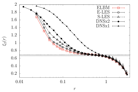


Which means that the models allows to save a factor in terms of the number of degrees of freedom required in the simulations. Considering that also the time-step needs to be changed accordingly in the higher resolution DNS to resolve the smaller time-scales, it means that the modelled simulations are more than an order of magnitude cheaper than a DNS with the same inertial range. On the other hand, by measuring the local scaling exponents as reported on the right column of Fig. 5, we can see that the inertial range extension produced by the model is not as accurate as the fully resolved DNS. This is a problem if we want the model to correctly describe intermittency. Let us stress that the correction to the K41 prediction at the level of the second and fourth order exponents is very small, hence a model needs to be extremely accurate to correctly capture the intermittent scaling biferale2019self . In both right panels of Fig. 5 we report with solid line the value of the K41 prediction, and with dotted lines the values measured from DNS as reported in Gotoh2002 ; sinhuber2017dissipative . To highlight intermittency we can look at the ratio between SF at different orders. In particular, any systematic non-linear dependency of vs , will introduce a scale-dependency in the Kurtosis, defined by the dimensionless ratio among fourth and second order SF,
| (23) |
In Fig. 6 we see that in all simulations, at large scales the increments are Gaussian (), while the Kurtosis quickly increases, decreasing the scale. This observation shows non-self similarity in the statistics of all data. It is interesting to observe that at this level the inertial range of scale observed in the DNSx2 simulation are well captured by all closures up to the dissipative scales where deviations from the DNSs and models arise.

Going further, we measure the most refined quantity we can observe to quantify intermittency, namely the local scaling exponent in Extended Self-Similarity Benzi1993 ,
| (24) |
A linear K41 behavior would recover in the inertial range a plateau value of equal to . The correction, accounting for intermittency, measured in both experimental and DNS data gives the plateau for at the value of Gotoh2002 ; sinhuber2017dissipative ; biferale2019self . As we can see in Fig. 7, all models show deviations from the K41 self-similar prediction meaning that they all capture the non-self-similarity of the turbulent inertial range. However none of them is really accurate enough to extend the length of the plateau displayed, hence to improve the prediction obtainable from the DNS at the same resolution. Indeed, if we compare the modelled data with the fully resolved simulations we can see that former are not showing any flat plateau in the inertial range and we cannot estimate precisely the correction to K41 of the structure function scaling exponents.

It is interesting to point out that the models show a very similar accuracy up to this last analysis. This suggest the backscatter events of energy introduced by the entropic closures are not accurate enough to improve quantitatively the statistics of the Smagorinsky model. This results supports the observation that intermittency in turbulent flows comes as a result of highly non-trivial correlations among all degrees of freedom at different scales buzzicotti2016phase ; buzzicotti2016lagrangian ; lanotte2015turbulence . The observation that for all models we have a very similar inertial range statistics goes in agreement with the common property of these models to have the same scaling, proportional to the strain rate tensor.
VI Conclusions
In this paper, we performed a quantitative assessment of the ELBM capabilities in the modelling of 3d homogeneous isotropic turbulent flows by comparing the inertial range statistics of ELBM data with the one of high resolution DNS of the NSE. We also compared the quality of ELBM with respect to the hydrodynamical Smagorinsky model, popular in the realm of LES. Furthermore, in this work we have proposed and investigated for the first time, a new hydrodynamical closure for LES simulation inspired from the macroscopic approximation of the ELBM model introduce by Malaspinas2008 . We found that ELBM extends the length of the inertial range with respect to the fully resolved DNS, allowing to reduce the computational cost by an order of magnitude and at the same time preserving the simulation stability. Results showed that, in both the macroscopic and mesoscopic formulations, ELBM is able to reproduce an inertial range with a non self-similar dynamics. ELBM captures the correct deviations from the large scales Gaussian statistics as observed in the fully resolved DNS, with an accuracy comparable to the one produced by the Smagorinsky model. From the measure of the structure functions scaling exponents in ESS, we have highlighted the limitations of these models to get with high accuracy the turbulence corrections to the Kolmogorov scaling. In this context we found that the modelled data are not producing the same inertial range plateau as observed in the fully resolved DNS and experiments. To conclude, we found that ELBM suffers in the modeling of extreme and rare intermittent fluctuations, while on the other hand it is very efficient in modeling the mean properties of 3d turbulence. Which makes ELBM a good candidate for the modeling of 3d turbulent flows in complex geometries.
Acknowledgement
The authors thank Prof. Luca Biferale for inspiration and many useful discussions. This work was supported also by the European Unions Framework Programme for Research and Innovation Horizon 2020 (2014-2020) under the Marie Skłodowska-Curie grant [grant number 642069] and by the European Research Council under the ERC grant [grant number 339032]. The authors would like to thanks Prof. Dirk Pleiter as well as the Juelich Supercomputing Center for providing access to the JURON cluster.
References
- [1] O. Malaspinas, M. Deville, and B. Chopard. Towards a physical interpretation of the entropic Lattice Boltzmann method. Physical Review E, 78(6):066705, 2008.
- [2] Horia Dumitrescu and Vladimir Cardos. Rotational effects on the boundary-layer flow in wind turbines. AIAA journal, 42(2):408–411, 2004.
- [3] P. A. Davidson. Turbulence: An Introduction for Scientists and Engineers. Oxford University Press, 2015.
- [4] S. B. Pope. Turbulent Flows. Cambridge University press, 2000.
- [5] Adrian E Gill. Atmosphere—ocean dynamics. Elsevier, 2016.
- [6] Alexandros Alexakis and Luca Biferale. Cascades and transitions in turbulent flows. Physics Reports, 767:1–101, 2018.
- [7] Sydney A Barnes. An assessment of the rotation rates of the host stars of extrasolar planets. The Astrophysical Journal, 561(2):1095, 2001.
- [8] U. Frisch. Turbulence : the legacy of A.N. Kolmogorov. Cambridge University Press, 1995.
- [9] Rodney O Fox. Computational models for turbulent reacting flows. Cambridge university press, 2003.
- [10] Takashi Ishihara, Toshiyuki Gotoh, and Yukio Kaneda. Study of high–reynolds number isotropic turbulence by direct numerical simulation. Annual Review of Fluid Mechanics, 41:165–180, 2009.
- [11] PK Yeung, XM Zhai, and Katepalli R Sreenivasan. Extreme events in computational turbulence. Proceedings of the National Academy of Sciences, 112(41):12633–12638, 2015.
- [12] R Benzi, L Biferale, R Fisher, D Lamb, and F Toschi. Inertial range eulerian and lagrangian statistics from numerical simulations of isotropic turbulence. 2010.
- [13] Kartik P Iyer, Katepalli R Sreenivasan, and PK Yeung. Reynolds number scaling of velocity increments in isotropic turbulence. Physical Review E, 95(2):021101, 2017.
- [14] C. Meneveau and J. Katz. Scale-invariance and turbulence models for large-eddy simulation. Annual Review of Fluid Mechanics, 32(1):1–32, 2000.
- [15] Olga Filippova, Sauro Succi, Francesco Mazzocco, Cinzio Arrighetti, Gino Bella, and Dieter Hänel. Multiscale lattice boltzmann schemes with turbulence modeling. Journal of Computational Physics, 170(2):812–829, 2001.
- [16] Y.-H. Dong and P. Sagaut. A study of time correlations in Lattice Boltzmann-based large-eddy simulation of isotropic turbulence. Physics of Fluids, 20(3):035105, 2008.
- [17] Y.-H. Dong, P. Sagaut, and S. Marie. Inertial consistent subgrid model for large-eddy simulation based on the Lattice Boltzmann method. Physics of Fluids, 20(3):035104, 2008.
- [18] Tomas Bohr, Mogens H Jensen, Giovanni Paladin, and Angelo Vulpiani. Dynamical systems approach to turbulence. Cambridge University Press, 2005.
- [19] M. Lesieur, O. Métais, and P. Comte. Large-eddy simulations of turbulence. Cambridge University Press, 2005.
- [20] Sybren Ruurds De Groot and Peter Mazur. Non-equilibrium thermodynamics. Courier Corporation, 2013.
- [21] Roberto Benzi, Sauro Succi, and Massimo Vergassola. The lattice boltzmann equation: theory and applications. Physics Reports, 222(3):145–197, 1992.
- [22] S. Succi. The Lattice Boltzmann Equation for Fluid Dynamics and Beyond. Oxford University Press, 2001.
- [23] Uriel Frisch, Brosl Hasslacher, and Yves Pomeau. Lattice-gas automata for the navier-stokes equation. Physical review letters, 56(14):1505, 1986.
- [24] D. A. Wolf-Gladrow. Lattice-gas cellular automata and Lattice Boltzmann models : an introduction. Springer, 2000.
- [25] Yue-Hong Qian, S Succi, and SA Orszag. Recent advances in lattice boltzmann computing. In Annual reviews of computational physics III, pages 195–242. World Scientific, 1995.
- [26] Shiyi Chen and Gary D Doolen. Lattice boltzmann method for fluid flows. Annual review of fluid mechanics, 30(1):329–364, 1998.
- [27] P. L. Bhatnagar, E. P. Gross, and M. Krook. A model for collision processes in gases. I. Small amplitude processes in charged and neutral one-component systems. Phys. Rev., 94:511–525, 1954.
- [28] G. Tauzin, L. Biferale, M. Sbragaglia, A. Gupta, F. Toschi, A. Bartel, and M. Ehrhardt. A numerical tool for the study of the hydrodynamic recovery of the Lattice Boltzmann method. Computers & Fluids, 172:241 – 250, 2018.
- [29] Jack GM Eggels. Direct and large-eddy simulation of turbulent fluid flow using the lattice-boltzmann scheme. International journal of heat and fluid flow, 17(3):307–323, 1996.
- [30] Huidan Yu, Li-Shi Luo, and Sharath S Girimaji. Les of turbulent square jet flow using an mrt lattice boltzmann model. Computers & Fluids, 35(8-9):957–965, 2006.
- [31] Pierre Sagaut. Toward advanced subgrid models for lattice-boltzmann-based large-eddy simulation: Theoretical formulations. Computers & Mathematics with Applications, 59(7):2194–2199, 2010.
- [32] Orestis Malaspinas and Pierre Sagaut. Consistent subgrid scale modelling for lattice boltzmann methods. Journal of Fluid Mechanics, 700:514–542, 2012.
- [33] I. V. Karlin, A. Ferrante, and H. C. Öttinger. Perfect entropy functions of the Lattice Boltzmann method. Europhysics Letters (EPL), 47(2):182–188, 1999.
- [34] Santosh Ansumali and Iliya V Karlin. Single relaxation time model for entropic lattice boltzmann methods. Physical Review E, 65(5):056312, 2002.
- [35] S. Ansumali, I. V. Karlin, and H. C. Öttinger. Minimal entropic kinetic models for hydrodynamics. Europhysics Letters (EPL), 63(6):798–804, 2003.
- [36] I. V. Karlin, F. Bösch, S. S. Chikatamarla, and S. Succi. Entropy-assisted computing of low-dissipative systems. Entropy, 17(12):8099–8110, 2015.
- [37] Benedikt Dorschner, Fabian Bösch, Shyam S Chikatamarla, Konstantinos Boulouchos, and Ilya V Karlin. Entropic multi-relaxation time lattice boltzmann model for complex flows. Journal of Fluid Mechanics, 801:623, 2016.
- [38] Benedikt Dorschner, Shyam S Chikatamarla, and Iliya V Karlin. Transitional flows with the entropic lattice boltzmann method. Journal of Fluid Mechanics, 824:388, 2017.
- [39] Benedikt Dorschner, Shyam S Chikatamarla, and Ilya V Karlin. Fluid-structure interaction with the entropic lattice boltzmann method. Physical Review E, 97(2):023305, 2018.
- [40] Ilya V Karlin, Fabian Bösch, and SS Chikatamarla. Gibbs’ principle for the lattice-kinetic theory of fluid dynamics. Physical Review E, 90(3):031302, 2014.
- [41] Fabian Bösch, Shyam S Chikatamarla, and Ilya V Karlin. Entropic multirelaxation lattice boltzmann models for turbulent flows. Physical Review E, 92(4):043309, 2015.
- [42] Guillaume Tauzin. Implicit Sub-Grid Scale Modeling within the Entropic Lattice Boltzmann Method in Homogeneous Isotropic Turbulence. PhD thesis, Universität Wuppertal, Fakultät für Mathematik und Naturwissenschaften …, 2019.
- [43] J. Smagorinsky. General circulation experiments with the primitive equations. 91(3):99–194, 1963.
- [44] Luca Biferale, Fabio Bonaccorso, Michele Buzzicotti, and Kartik P Iyer. Self-similar subgrid-scale models for inertial range turbulence and accurate measurements of intermittency. Physical review letters, 123(1):014503, 2019.
- [45] A. Arnèodo, R. Benzi, J. Berg, L. Biferale, E. Bodenschatz, A. Busse, E. Calzavarini, B. Castaing, M. Cencini, L. Chevillard, R. T. Fisher, R. Grauer, H. Homann, D. Lamb, A. S. Lanotte, E. Lévèque, B. Lüthi, J. Mann, N. Mordant, W.-C. Müller, S. Ott, N. T. Ouellette, J.-F. Pinton, S. B. Pope, S. G. Roux, F. Toschi, H. Xu, and P. K. Yeung. Universal intermittent properties of particle trajectories in highly turbulent flows. Phys. Rev. Lett., 100:254504, 2008.
- [46] M Buzzicotti, M Linkmann, H Aluie, L Biferale, J Brasseur, and C Meneveau. Effect of filter type on the statistics of energy transfer between resolved and subfilter scales from a-priori analysis of direct numerical simulations of isotropic turbulence. Journal of Turbulence, 19(2):167–197, 2018.
- [47] A Leonard et al. Energy cascade in large-eddy simulations of turbulent fluid flows. Adv. Geophys. A, 18(A):237–248, 1974.
- [48] T. Krüger, H. Kusumaatmaja, A. Kuzmin, O. Shardt, G. Silva, and E. M. Viggen. The Lattice Boltzmann Method. Graduate Texts in Physics. Springer International Publishing, Cham, 2017.
- [49] A. L. Kuperstokh. New method of incorporating a body force term into the Lattice Boltzmann equation. In Proceedings of the 5th International EDH Workshop, pages 241–246, Poitiers, France, 2004.
- [50] Michele Buzzicotti and Patricio Clark Di Leoni. Synchronizing subgrid scale models of turbulence to data. Physics of Fluids, 32(12):125116, 2020.
- [51] G. S. Patterson and S. A. Orszag. Spectral Calculations of Isotropic Turbulence: Efficient Removal of Aliasing Interactions. Phys. Fluids, 14:2538–2541, 1971.
- [52] V. Borue and S. A. Orszag. Self-similar decay of three-dimensional homogeneous turbulence with hyperviscosity. Phys. Rev. E, 51:2859(R), 1995.
- [53] Toshiyuki Gotoh and Takeshi Watanabe. Statistics of transfer fluxes of the kinetic energy and scalar variance. Journal of Turbulence, (6):N33, 2005.
- [54] Michele Buzzicotti, Hussein Aluie, Luca Biferale, and Moritz Linkmann. Energy transfer in turbulence under rotation. Physical Review Fluids, 3(3):034802, 2018.
- [55] A. N. Kolmogorov. The local structure of turbulence in incompressible viscous fluid for very large Reynolds numbers. In Dokl. Akad. Nauk SSSR, volume 30, pages 301–305. JSTOR, 1941.
- [56] T. Gotoh, D. Fukayama, and T. Nakano. Velocity field statistics in homogeneous steady turbulence obtained using a high-resolution direct numerical simulation. Physics of Fluids (1994-present), 14(3):1065–1081, 2002.
- [57] Michael Sinhuber, Gregory P Bewley, and Eberhard Bodenschatz. Dissipative effects on inertial-range statistics at high reynolds numbers. Physical review letters, 119(13):134502, 2017.
- [58] R. Benzi, S. Ciliberto, R. Tripiccione, C. Baudet, F. Massaioli, and S. Succi. Extended self-similarity in turbulent flows. Phys. Rev. E, 48:R29–R32, 1993.
- [59] Michele Buzzicotti, Brendan P Murray, Luca Biferale, and Miguel D Bustamante. Phase and precession evolution in the burgers equation. The European Physical Journal E, 39(3):1–9, 2016.
- [60] Michele Buzzicotti, Akshay Bhatnagar, Luca Biferale, Alessandra S Lanotte, and Samriddhi Sankar Ray. Lagrangian statistics for navier–stokes turbulence under fourier-mode reduction: fractal and homogeneous decimations. New Journal of Physics, 18(11):113047, 2016.
- [61] Alessandra S Lanotte, Roberto Benzi, Shiva K Malapaka, Federico Toschi, and Luca Biferale. Turbulence on a fractal fourier set. Physical review letters, 115(26):264502, 2015.