Indicators of Attack Failure: Debugging and Improving Optimization of Adversarial Examples

Maura Pintor
University of Cagliari, Italy
Pluribus One, Italy
[email protected] &Luca Demetrio
University of Genoa, Italy
Pluribus One, Italy
[email protected] Angelo Sotgiu
University of Cagliari, Italy
[email protected] &Ambra Demontis
University of Cagliari, Italy
[email protected] &Nicholas Carlini
Google
[email protected] Battista Biggio
University of Cagliari, CINI, Italy
Pluribus One, Italy
[email protected] &Fabio Roli
University of Genoa, CINI, Italy
Pluribus One, Italy
[email protected]

Abstract

Evaluating robustness of machine-learning models to adversarial examples is a challenging problem. Many defenses have been shown to provide a false sense of robustness by causing gradient-based attacks to fail, and they have been broken under more rigorous evaluations. Although guidelines and best practices have been suggested to improve current adversarial robustness evaluations, the lack of automatic testing and debugging tools makes it difficult to apply these recommendations in a systematic manner. In this work, we overcome these limitations by: (i) categorizing attack failures based on how they affect the optimization of gradient-based attacks, while also unveiling two novel failures affecting many popular attack implementations and past evaluations; (ii) proposing six novel indicators of failure, to automatically detect the presence of such failures in the attack optimization process; and (iii) suggesting a systematic protocol to apply the corresponding fixes. Our extensive experimental analysis, involving more than 15 models in 3 distinct application domains, shows that our indicators of failure can be used to debug and improve current adversarial robustness evaluations, thereby providing a first concrete step towards automatizing and systematizing them. Our open-source code is available at: https://github.com/pralab/IndicatorsOfAttackFailure.

1 Introduction

Despite their unprecedented success in many different applications, machine-learning models have been shown to be vulnerable to adversarial examples [40, 4], i.e., inputs intentionally crafted to mislead such models at test time. While hundreds of defenses have been proposed to overcome this issue [46, 29, 43, 36], many of them turned out to be ineffective, as their robustness to adversarial inputs was significantly overestimated. In particular, some defenses were evaluated by running existing attacks with inappropriate hyperparameters (e.g., using an insufficient number of iterations), while others were implicitly obfuscating gradients, thereby causing the optimization of gradient-based attacks to fail. Such defenses have been shown to yield much lower robustness under more rigorous robustness evaluations and using attacks carefully adapted to evade them [10, 2].

To prevent such evaluation mistakes, and help develop better defenses, evaluation guidelines and best practices have been described in recent work [11]. However, they have been mostly neglected as their application is non-trivial; in fact, 13 defenses published after the release of these guidelines were found again to be wrongly evaluated, reporting overestimated adversarial robustness values [41]. It has also been shown that, even when following such guidelines, robustness can still be overestimated [33]. Finally, while recently-proposed frameworks combining diverse attacks seem to provide more reliable adversarial robustness evaluations [13, 44], it is still unclear whether and to what extent the considered attacks can also be affected by subtle failures.

To address these limitations, in this work we propose the first testing approach aimed to debug and automatically detect misleading adversarial robustness evaluations. The underlying idea, similar to traditional software testing, is to lower the entry barrier for researchers and practitioners towards performing more reliable robustness evaluations. To this end, we provide the following contributions: (i) we categorize four known attack failures by connecting them to the optimization process of gradient-based attacks, which enabled us also to identify two additional, never-before-seen failures affecting many popular attack implementations and past evaluations (Sect. 2.1); (ii) we propose six indicators of attack failures (IoAF), i.e., quantitative metrics derived by analyzing the optimization process of gradient-based attacks, which can automatically detect the corresponding failures (Sect. 2.2); and (iii) we suggest a systematic, semi-automated protocol to apply the corresponding fixes (Sect. 2.3). We empirically validate our approach on three distinct application domains (images, audio, and malware), showing how recently-proposed, wrongly-evaluated defenses could have been evaluated correctly by monitoring the IoAF values and following our evaluation protocol (Sect. 3). We also open source our code and data to enable reproducibility of our findings at https://github.com/pralab/IndicatorsOfAttackFailure. We conclude by discussing related work (Sect. 4), limitations, and future research directions (Sect. 5).

2 Debugging Adversarial Robustness Evaluations

We introduce here our automated testing approach for adversarial robustness evaluations, based on the design of novel metrics, referred to as Indicators of Attack Failure (IoAF), each aimed to detect a specific failure within the optimization process of gradient-based attacks.

2.1 Optimizing Gradient-based Attacks

Before introducing the IoAF, we discuss how gradient-based attacks are optimized, and provide a generalized attack algorithm that will help us to identify the main attack failures. In particular, we consider attacks that solve the following optimization problem:

	$\displaystyle\min_{\boldsymbol{\delta}}$		$\displaystyle L(\boldsymbol{x}+\boldsymbol{\delta},y_{t};\boldsymbol{\theta}),$		(1)
	$\displaystyle{\rm s.t.}$		$\displaystyle\\|\boldsymbol{\delta}\\|_{p}\leq\epsilon,\;\;{\rm and}\;\;\;\boldsymbol{x}+\boldsymbol{\delta}\in[0,1]^{d},$		(2)

where $\boldsymbol{x}\in[0,1]^{d}$ is the $d$ -dimensional input sample, $y_{t}\in\mathcal{Y}=\{1,\ldots,c\}$ is the target class label (chosen to be different from the true label $y$ of the input sample), $\boldsymbol{\delta}\in\mathbb{R}^{d}$ is the perturbation applied to the input sample during the optimization, and $\boldsymbol{\theta}$ are the parameters of the model. The loss function $L$ is defined such that minimizing it amounts to having the perturbed sample $\boldsymbol{x}+\boldsymbol{\delta}$ misclassified as $y_{t}$ . Typical examples include the Cross-Entropy (CE) loss, or the so-called logit loss [10], i.e., $L(\boldsymbol{x}+\boldsymbol{\delta},y_{t},\boldsymbol{\theta})=\max_{k\neq y_{t}}f_{k}(\boldsymbol{x}+\boldsymbol{\delta},\boldsymbol{\theta})-f_{y_{t}}(\boldsymbol{x}+\boldsymbol{\delta},\boldsymbol{\theta})$ , being $f_{i}(\cdot,\boldsymbol{\theta})$ the model’s prediction (logit) for class $i$ .¹¹1Note that, while Eq. (1) describes targeted attacks, untargeted attacks can be easily accounted for by substituting $y_{t}$ with $y$ and changing the sign of $L$ . Let us finally discuss the constraints in Eq. (2). While the $\ell_{p}$ -norm constraint $\|\boldsymbol{\delta}\|_{p}\leq\epsilon$ bounds the maximum perturbation size, the box constraint $\boldsymbol{x}+\boldsymbol{\delta}\in[0,1]^{d}$ ensures that the perturbed sample stays withing the given (normalization) bounds.

Transfer Attacks. When the target model is either non-differentiable or not sufficiently smooth [2], a surrogate model $\hat{\boldsymbol{\theta}}$ can be used to provide a smoother approximation of the loss $L$ , and facilitate the attack optimization. The attack is thus optimized on the surrogate model, and then evaluated against the target model. If the attack is successful, then it is said to correctly transfer to the target [30].

Input :

\boldsymbol{x}

, the initial sample;

y_{t}

, the target class label;

n

, the number of iterations;

\alpha

, the step size;

\boldsymbol{\theta}

, the target model;

L

the loss function;

\Pi

, the projection operator enforcing the constraints in Eq. (2).

Output :

\boldsymbol{x}^{\star}

, the solution found by the algorithm

\boldsymbol{x}_{0}\leftarrow

initialize

(\boldsymbol{x})

\triangleright

Initialize starting point

\hat{\boldsymbol{\theta}}\leftarrow

approximation

(\boldsymbol{\theta})

\triangleright

Use surrogate model (if required)

\boldsymbol{\delta}_{0}\leftarrow\boldsymbol{0}

\triangleright

Initialize

\delta

1 for $i\in[1,n]$ do

\boldsymbol{\delta}_{i}\leftarrow\boldsymbol{\delta}_{i-1}-\alpha\nabla_{\boldsymbol{x}}L(\boldsymbol{x}+\boldsymbol{\delta}_{i-1},y_{t};\hat{\boldsymbol{\theta}})

\triangleright

Compute gradient update(s)

\boldsymbol{\delta}_{i}\leftarrow\Pi(\boldsymbol{x},\boldsymbol{\delta}_{i})

\triangleright

Project

\boldsymbol{\delta}

onto the feasible domain (Eq. 2)

return

\boldsymbol{x}^{\star}\leftarrow

\boldsymbol{x}

+ best

(\boldsymbol{\delta}_{0},...,\boldsymbol{\delta}_{n})

\triangleright

Return best solution

Algorithm 1 Generalized gradient-based attack for optimizing adversarial examples.

Generalized Attack Algorithm. We provide here a generalized algorithm, given as Algorithm 1, which summarizes the main steps followed by gradient-based attacks to solve Problem (1)-(2). The algorithm starts by defining an initialization point (line 1), which can be the input sample $\boldsymbol{x}$ , a randomly-perturbed version of it, or even a sample from the target class [5]. If the target model $\boldsymbol{\theta}$ is either non-differentiable or not sufficiently smooth, a surrogate model $\hat{\boldsymbol{\theta}}$ can be used to approximate it, and perform a transfer attack (line 1). The attack then iteratively updates the point to find an adversarial example (line 1), computing one (or more) gradient updates in each iteration (line 1), while the perturbation $\boldsymbol{\delta}_{i+1}$ is projected onto the feasible domain (i.e., the intersection of the constraints in Eq. 2) via a projection operator $\Pi$ (line 1). The algorithm finally returns the best perturbation across the whole attack path, i.e., the perturbed sample that evades the (target) model with the lowest loss (line 1). This generalized attack algorithm provides the basis for identifying known and novel attack failures, by connecting each failure to a specific step of the algorithm, as discussed in the next section.

Other Perturbation Models. We conclude this section by remarking that, even if we consider additive $\ell_{p}$ -norm perturbations in our formulation, the proposed approach can be easily extended to more general perturbation models (e.g., represented as $\boldsymbol{x}^{\prime}=h(\boldsymbol{x},\boldsymbol{\delta})$ , being $\boldsymbol{x}^{\prime}$ the perturbed feature representation of a valid input sample, and $h$ a manipulation function parameterized by $\boldsymbol{\delta}$ , as in [17]). In fact, our approach can be used to debug and evaluate any attack as long as it is optimized via gradient descent, regardless of the given perturbation model and constraints, as also demonstrated in our experiments (A.3,A.4, A.5).

2.2 Indicators of Attack Failure

We introduce here our approach, compactly represented in Fig. 1, by describing the identified attack failures, along with the corresponding indicators and mitigation strategies. We describe two main categories of failures, respectively referred to as loss-landscape and attack-optimization failures.

Loss-landscape Failures, Mitigations, and Indicators. The first category of failures depends on the choice of the loss function $L$ and of the target model $\boldsymbol{\theta}$ , regardless of the specific attack implementation. In fact, it has been shown that the objective function in Eq. (1) may exhibit obfuscated gradients [10, 2], which prevent gradient-based attacks to find adversarial examples even when they exist within the feasible domain. We report two known failures linked to this issue, referred as F₁ and F₂ below.
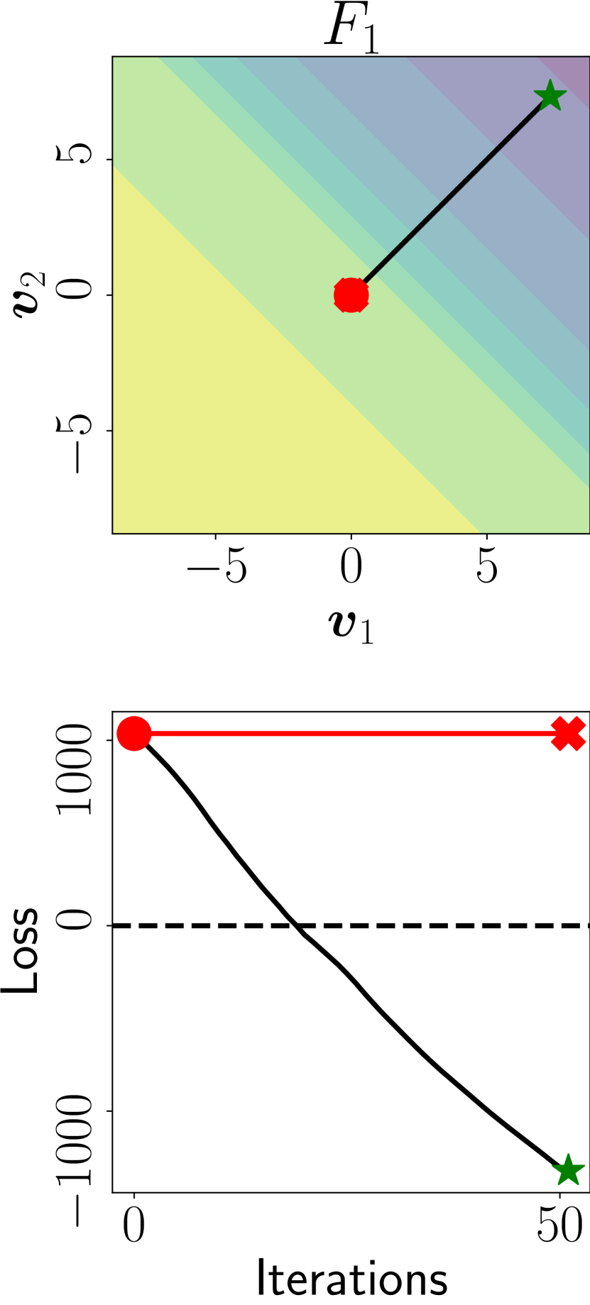
F₁: Shattered Gradients. This failure is reported in [3, 8]. It compromises the computation of the input gradient $\nabla_{\boldsymbol{x}}L$ , and the whole execution of the attack, when at least one of the model’s components (e.g., a specific layer) is non-differentiable or causes numerical instabilities (F₁ in Fig. 3).
M₁: Use BPDA. This failure can be overcome using the Backward Pass Differentiable Approximation (BPDA) [3, 41], i.e., replacing the derivative of the problematic components with the identity matrix.
I₁: Unavailable Gradients. Despite the failure and mitigation being known, no automated, systematic approach has ever been proposed to detect F₁. This newly-proposed indicator is able to automatically detect the presence of non-differentiable components and numerical instabilities when computing gradients; in particular, for each given input $\boldsymbol{x}$ , if the input gradient $\nabla_{\boldsymbol{x}}L(\boldsymbol{x},y_{t},\boldsymbol{\theta})$ has zero norm, or if its computation returns an error, we set $I_{1}(\boldsymbol{x})=1$ (and $0$ otherwise).

F₂: Stochastic Gradients. This failure is reported in [2, 41]. The input gradients can be computed, but their value is uninformative, as following the gradient direction does not correctly minimize the loss function $L$ . Such issue arises when models introduce randomness in the inference process [22], or when their training induces noisy gradients [43] (F₂ in Fig. 3).
M₂: Use EoT. Previous work mitigates this failure using Expectation over Transformation (EoT) [2, 41], i.e., by averaging the loss $L$ over the same transformations performed by the randomized model, or over random perturbations of the input (sampled from a given distribution).
I₂: Unstable Predictions. Despite the failure and mitigation being known, no automated, systematic approach has been considered to automatically detect F₂. This novel indicator measures the relative variability $V(\boldsymbol{x})$ of the loss function $L$ around the input samples. Given an input sample $\boldsymbol{x}$ , we draw $s$ perturbed inputs uniformly from a small $\ell_{2}$ ball centered on $\boldsymbol{x}$ , with radius $r$ , and compute $V(\boldsymbol{x})=\min(\frac{1}{s}\sum_{i=1}^{s}|(L_{0}-L_{i})/L_{0}|,1)\in[0,1]$ , where $L_{0}$ is the loss obtained at $\boldsymbol{x}$ , $L_{1},...,L_{s}$ are the loss values computed on the perturbed samples, and the $\min$ operator is used to upper bound $V(\boldsymbol{x})\leq 1$ . We then set $I_{2}(\boldsymbol{x})=1$ if $V(\boldsymbol{x})\geq\tau$ (and $0$ otherwise). In our experiments, we set the parameters of this indicator as $s=100$ , $r=10^{-}3$ and $\tau=10\%$ , as explained in Sect. 3.

Refer to caption — Figure 1: Indicators of Attack Failure (IoAF). We show the connections among the distinct attack failures (top), the proposed IoAF (center), and the corresponding mitigations (bottom). The novel failures, indicators, and mitigations found in this work are highlighted in bold and marked with “ $\ast$ ”.

Attack-optimization Failures, Mitigations, and Indicators. The second category of failures is connected to problems encountered when running a gradient-based attack to solve Problem (1)-(2) with Algorithm 1. This category encompasses failures $F_{3}$ - $F_{6}$ in Fig. 3.
F₃: Implementation Errors. We are the first to identify and characterize this failure, which affects many widely-used attack implementations and past evaluations. In particular, we find that many attacks return the last sample of the attack path (line 1 of Algorithm 2.1) even if it is not adversarial, discarding valid adversarial examples found earlier in the attack path (F₃ in Fig. 3). This issue affects: (i) the PGD attack implementations [25] currently used in the four most-used Python libraries for crafting adversarial examples, i.e., Foolbox, CleverHans, ART, and Torchattacks (for further details, please refer to A.6); and also (ii) AutoAttack [13], as it returns the initial sample if no adversarial example is found, leading to flawed evaluations when used in transfer settings [15].
M₃: Fix Attack Implementation. To fix the issue, we propose to modify the optimization algorithm to return the best result. This mitigation can also be automated using the same mechanism used to automatically evaluate the IoAF, i.e., by wrapping the attack algorithm with a function that keeps track of the best sample found during the attack optimization and eventually returns it.
I₃: Silent Success. We design $I_{3}(\boldsymbol{x})$ as a binary indicator that is set to $1$ when the final point in the path is not adversarial, but an adversarial example is found along the attack path (and $0$ otherwise).

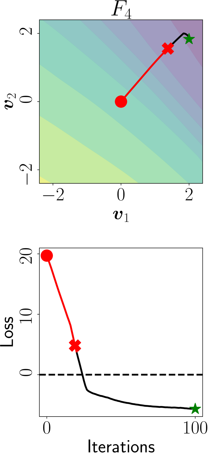
F₄: Non-converging Attack. This failure is reported in [41], noting that the flawed evaluations performed by Buckman et al. [6] and Pang et al. [28], respectively, used only 7 and 10 steps of PGD for testing their defenses. More generally, attacks may not reach convergence (F₄ in Fig. 3) due to inappropriate choices of their hyperparameters, including not only an insufficient number of iterations $n$ (line 1 of Algorithm 1), but also an inadequate step size $\alpha$ (line 1 of Algorithm 1).

M₄: Tune Step Size and Iterations. The failure can be patched by increasing either the step size $\alpha$ or the number of iterations $n$ .
I₄: Incomplete Optimization. To automatically evaluate if the attack has not converged, we propose a novel indicator that builds a monotonically decreasing curve $\hat{L}$ for the loss, by keeping track of the best minimum found at each attack iteration (a.k.a. cumulative minimum curve, shown in black in Fig. 2). Then, we compute the relative loss decrement $D(\boldsymbol{x})$ in the last $k$ iterations (out of $n$ ) as: $D(\boldsymbol{x})=|\hat{L}^{(n)}-\hat{L}^{(n-k)}|/(\max_{i}\hat{L}^{(i)}-\min_{i}\hat{L}^{(i)})\in[0,1]$ . We set $I_{4}(\boldsymbol{x})=1$ if $D(\boldsymbol{x})\geq\mu$ (and 0 otherwise). In our experiments, we set the parameters $k=10$ and $\mu=1\%$ , as detailed in Sect. 3.

F₅: Non-adaptive attack. This failure is only qualitatively discussed in [3, 11, 41], showing that many previously-published defenses can be broken by developing adaptive attacks that specifically target the given defense mechanism. However, to date, it is still unclear how to evaluate if an attack is really adaptive or not (as it is mostly left to a subjective judgment). We try to shed light on this issue below. We first note that this issue arises when existing attacks are executed against defenses that may either have non-differentiable components [16] or use additional detection mechanisms [26]. In both cases, the attack is implicitly executed in a transfer setting against a surrogate model which retains the main structure of the target, but ignores the problematic components/detectors; e.g., Das et al. [16] simply removed the JPEG compression component from the model. However, it should be clear that optimizing the attack against such a bad surrogate $\hat{\boldsymbol{\theta}}$ (line 1 of Algorithm 1) is not guaranteed to also bypass the target model $\boldsymbol{\theta}$ (F₅ in Fig. 3).
M₅: Change Loss (Adaptive). Previous work [3, 11, 41] applied custom fixes by using better approximations of the target, i.e., loss functions and surrogate models that consider all the components of the defense in the attack optimization. This is unfortunately a non-trivial step to automate.
I₅: Transfer Failure. Despite the failure and some qualitative ideas to implement mitigations being known, it is unclear how to measure and evaluate if an attack is really adaptive. To this end, we propose an indicator that detects F₅ by evaluating the misalignment between the loss $L$ optimized by the attack on the surrogate $\hat{\boldsymbol{\theta}}$ and the same function evaluated on the target $\boldsymbol{\theta}$ . We thus set $I_{5}(\boldsymbol{x})=1$ if the attack sample bypasses the surrogate but not the target model (and $0$ otherwise).

F₆: Unreachable Misclassification. We are the first to identify and characterize this failure. It assumes that gradient-based attacks can get stuck in bad local minima (e.g., characterized by flat regions), where no adversarial example is found (F₆ in Fig. 3). When this failure is present, unconstrained attacks (i.e., attacks with $\epsilon\rightarrow\infty$ in Eq. 2) are also expected to fail, even if adversarial examples exist for sure in this setting (since the feasible domain includes samples from all classes).
M₆: Change Loss (Bad Local Minimum). We argue that this failure can be fixed by modifying the loss function optimized by the attack, to avoid attack paths that lead to bad local minima. However, similarly to M₅, this is not a trivial issue to fix, and it is definitely not easy to automate.
I₆: Unconstrained Attack Failure. Despite being difficult to find a suitable mitigation for F₆, detecting it is straightforward. To this end, we run an unconstrained attack on the given input $\boldsymbol{x}$ , and we set $I_{6}(\boldsymbol{x})=1$ if such an attack fails (and $0$ otherwise).

2.3 How to Use Our Framework

We summarize here the required steps that developers and practitioners should follow to debug their robustness evaluations with our IoAF.

•

Initialize Evaluation. The evaluation is initialized with a chosen attack, along with its hyperparameters, number of samples, and the model to evaluate.
•

Mitigate Loss-landscape Failures. Before computing the attack, the evaluation should get rid of loss-landscape failures, by computing I₁ and I₂, and applying M₁ and M₂ accordingly. These indicators are computed on a small random subset of $N$ samples, as the presence of either F₁ or F₂ would render useless the execution of the attack on all points. Both F₁ and F₂ are reported if they are detected on at least one sample in the given subset.
•

Run the Attack. If F₁ and F₂ are absent or have been fixed, the attack can be run on all samples.
•

Mitigate Attack-specific Failures. Once the attack completes its execution, indicators I₃, I₄ and I₅ should be checked. Depending on their output, M₃, M₄, and M₅ are applied, and the attack is repeated (on the affected samples). If no failures are found, but the attack is still failing, the value of I₆ should be checked, and M₆ applied if needed. As I₁ and I₂, I₆ is also computed on a subset of $N$ samples to avoid unnecessary computations. The failure is reported if $\textit{I\textsubscript{6}}=1$ for at least one sample.

Let us finally remark that when no indicator triggers, one should not conclude that robustness may not be worsened by a different, more powerful attack. This is indeed a problem of any empirical evaluation, including software testing – which does not ensure that software is bug-free, but only that some known issues get fixed. Our methodology, similarly, highlights the presence of known failures in adversarial robustness evaluations and suggests how to mitigate them with a systematic protocol, taking a first concrete step toward making robustness evaluations more systematic and reliable.

3 Experiments

In this section, we demonstrate the effectiveness of our approach by re-evaluating the robustness of $7$ defenses, and using our IoAF framework to fix them. Additionally, we evaluate 6 more robust image classification models from a widely-used benchmark, discovering that their robustness claims might be unreliable. We also conduct the following additional experiments, reported in the appendix: (i) we describe how we set the thresholds $\tau$ for I₂ and $\mu$ for I₄ in A.2; and (ii) we offer evidence that IoAF can encompass perturbation models beyond $\ell_{p}$ norms by analyzing the robustness evaluations of one Windows malware detector in A.3, one Android malware detector in A.4, and one audio keyword-spotting model in A.4.

Experimental Setup. We run our attacks on an Intel^® Xeon^® CPU E5-2670 v3, with 48 cores, 128 GB of RAM, equipped with a Nvidia Quadro M6000 with 24 GB of memory, and we leverage the SecML library [32] to implement our methodology. We show failures of gradient-based attacks on 7 previously published defenses [16, 22, 29, 43, 28, 45, 38, 21, 47], by inspecting them with our IoAF, and most of them [16, 22, 29, 43, 28, 45] are characterized by wrong robustness evaluations. We choose these defenses because it is known that their original evaluations are incorrect [2, 41]; our goal here is to show that IoAF would have identified and mitigated such errors. We include the evaluation of an adversarial detector [38] to highlight that IoAF is able to detect possible failures of this family of classifiers. We include the robustness evaluations of a Wide-ResNet [47] and an adversarially-trained model [21], to highlight that our indicators do not trigger when they inspect sound evaluations. We defer details of the selected original evaluations to A.1. Lastly, to demonstrate that automated attacks do not provide guarantees on performing correct evaluations (without human intervention), we apply the AutoPGD attack [13] with Cross-Entropy loss (APGD_CE) and the Difference of Logits Ratio (APGD_DLR). Robustness is computed with the robust accuracy (RA) metric, quantified as the ratio of samples classified correctly within a given perturbation bound $\epsilon$ . For I₁, I₂, and I₆ we set $N=10$ , and for I₄ we set $k=10$ . For I₂, we set the number of sampled neighboors $s=100$ , and the radius of the $\ell_{2}$ ball $r=10^{-3}$ , to match the step size $\alpha$ of the evaluations. The thresholds $\tau$ of I₂ and $\mu$ of I₄ are set to $10\%$ and $1\%$ respectively (details about their calibration in A.2). All the robustness evaluations are performed on 100 samples from the test dataset of the considered model, and for each attack we evaluate the robust accuracy with $\epsilon=8/255$ for CIFAR models, and $\epsilon=0.5$ for the MNIST ones. The step size $\alpha$ is set to match the original evaluations (as detailed in A.1).

Table 1: Indicator values (cols.) computed on the selected models (rows) using different attacks. The robust accuracy (RA) is reported in the last column (best values in bold). The symbol "Tr" denotes a transfer attack. The

\checkmark

represents the detection of a specific failure. We report in parentheses the fraction of samples for which indicators I₂, I₃, I₄, and I₆ are active.

Model	Attack	I₁	I₂	I₃	I₄	I₅	I₆	RA
ST	PGD							0.00
ADV-T	PGD							0.48
DIST	Original	$\checkmark$					$\checkmark$ (10/10)	0.95
	APGD_CE	$\checkmark$					$\checkmark$ (10/10)	0.99
	APGD_DLR							0.00
	Patched							0.01
k-WTA	Original		$\checkmark$ (10/10)	$\checkmark$ (23%)	$\checkmark$ (11%)		$\checkmark$ (4/10)	0.67
	APGD_CE		$\checkmark$ (10/10)		$\checkmark$ (21%)		$\checkmark$ (2/10)	0.35
	APGD_DLR		$\checkmark$ (10/10)				$\checkmark$ (4/10)	0.28
	Patched				$\checkmark$ (6%)		$\checkmark$ (2/10)	0.09
IT	Original		$\checkmark$ (10/10)	$\checkmark$ (33%)	$\checkmark$ (90%)			0.32
	APGD_CE		$\checkmark$ (10/10)	$\checkmark$ (3% )			$\checkmark$ (2/10)	0.12
	APGD_DLR		$\checkmark$ (10/10)	$\checkmark$ (5%)			$\checkmark$ (1/10)	0.12
	Patched				$\checkmark$ (3%)			0.00
EN-DV	Original				$\checkmark$ (100%)		$\checkmark$ (3/10)	0.48
	APGD_CE							0.00
	APGD_DLR							0.00
	Patched							0.00
TWS	Original				$\checkmark$ (74%)	$\checkmark$ (6%)	$\checkmark$ (8/10)	0.77
	APGD_CE							0.03
	APGD_DLR						$\checkmark$ (7/10)	0.68
	Patched				$\checkmark$ (1%)			0.01
JPEG-C	Original	$\checkmark$						0.85
	Original (Tr)					$\checkmark$ (78%)		0.74
	APGD_CE (Tr)					$\checkmark$ (62%)		0.51
	APGD_DLR (Tr)					$\checkmark$ (85%)		0.70
	Patched							0.01
DNR	Original				$\checkmark$ (100%)		$\checkmark$ (10/10)	0.75
	APGD_CE				$\checkmark$ (3%)			0.02
	APGD_DLR						$\checkmark$ (2/10)	0.20
	Patched				$\checkmark$ (1%)			0.03

Identifying and Fixing Attack Failures. We now delve into the description of the considered evaluations, which failures we detect and how we mitigate them, reporting the results in Table 1.

Correct Evaluations (ST, ADV-T). We first evaluate the robustness analysis of the Wide-ResNet and the adversarially-trained model, by applying PGD with CE loss, with $n=100$ (number of steps) and $\alpha=0.03$ (step size). Since no gradient obfuscation techniques have been used, the loss landscape indicators do not trigger. Also, since the attacks smoothly converge, these evaluations do not trigger any attack optimization indicator. Their robust accuracy is, respectively, 0% and 48%.

Defensive Distillation (DIST). Papernot et al. [29] use distillation to train a classifier to saturate the last layer of the network, making the computations of gradients numerically unstable and impossible to calculate, triggering the I₁ indicator, but also I₆ indicator as the optimizer can not explore the space. To patch this evaluation, we apply M₁ to overcome the numerical instability caused by DIST, forcing the attack to leverage the logits of the model instead of computing the softmax. Such a fix reduces the robust accuracy from 95% to 1%. In contrast, APGD_DLR manages to decrease the robust accuracy to 0%, as it avoids the saturation issue by considering only the logits of the model, while APGD_CE triggers the same issues of the original evaluation.

k-Winners Take All (k-WTA). Xiao et al. [43] develop a classifier with a very noisy loss landscape, that destroys the meaningfulness of the directions of computed gradients. The original evaluation triggers I₂, since the loss landscape is characterized by frequent fluctuations, but also I₃, as the applied PGD [25] returns the last point of the attack discarding adversarial examples found within the path. Moreover, due to the noise, the attack is not always reaching convergence, as signaled by I₄, also performing little exploration of the space, as flagged by I₆. Hence, we apply M₂, performing EoT on the PGD loss, sampling 2000 points from a Normal distribution $\mathcal{N}(0,\sigma^{2}\mathbf{I})$ , with $\sigma=8/255$ . We fix the implementation with M₃, and increase the iterations with M₄, thus reducing the robust accuracy from 67% to 9%. However, our evaluation still triggers I₄ and I₆, implying that for some points the result can be improved further by increasing the number of steps or the smoothing parameter $\gamma$ . Both APGD_CE and APGD_DLR trigger I₂, since they are not applying EoT, and they partially activate I₆, similarly to the original evaluation. Interestingly, APGD_DLR converges better than APGD_CE, as the latter triggers I₄. Both attacks decrease the robust accuracy to 35% and 28%, a worst estimate than the one computed with the patched attack that directly handles the presence of the gradient obfuscation.

Input Transformations (IT). Guo et al. [22] apply random affine input transformations to input images, producing a noisy loss landscape that varies at each prediction, thus its original robustness evaluation I₂, I₃, and I₄ indicators, for the same reasons of k-WTA. Again, we apply M₂, M₃ and M₄, using EoT with $\gamma=200$ and $\sigma=8/255$ , decreasing the robust accuracy from 32% to 0%. Still, for some points (even if adversarial) the objective could still be improved, as I₄ is active for them. Both APGD_CE and APGD_DLR are able to slightly decrease the robust accuracy to 12%, but they both trigger the I₂ and I₆ indicator since they are not addressing the high variability of the loss landscape.

Ensemble Diversity (EN-DV). Pang et al. [28] propose an ensemble model, evaluated with only 10 steps of PGD, thus triggers the I₅ indicator since the attack is not reaching convergence. As a consequence, also the unbounded attack is failing, thus triggering I₆. We apply the M₄ mitigation and we set $n=100$ , as already done by previous work [41]. This fix changes the robust accuracy from 48% to 0%. Not surprisingly, both APGD_CE and APGD_DLR are able to bring the robust accuracy to 0%, since they both automatically modulate the step size.

Turning a Weakness into a Strength (TWS). Yu et al. [45] propose an adversarial example defense, composed of different detectors. For simplicity, we only consider one of these, and we repeat their original evaluation with PGD without the normalization operation on the computed gradients, and $n=50$ . This attack does not converge, triggering I₄, and if fails to navigate the loss landscape due to the very small gradients, triggering also I₆. We apply M₄, by setting $n=100$ , and we use the original implementation of PGD (with the normalization step), hence applying also M₆, achieving a drop in the robust accuracy from 77% to 1%. For only one point, our evaluation triggers I₄, as better convergence could be achieved. Moving forward, APGD_CE finds a robust accuracy of 3%, as it is modulating the step size along with using the normalization of the gradient. On the other hand, APGD_DLR triggers the I₆ indicator and the robust accuracy remains at 68%, as the attack is not able to avoid the rejection applied by the model.

JPEG Compression (JPEG-C). Das et al. [16] pre-process all input samples using JPEG compression, before feeding the input to the undefended network. We apply this defense on top of a model with a reverse sigmoid layer [23], as was done in [44]. The authors firstly state that they can not directly attack the defense due to its non-differentiability (thus triggering I₁), then they apply the DeepFool [27] attack against the undefended model. This attack has low transferability, as it is not maximizing the misclassification confidence [18]. The robustness evaluation triggers I₅ since the attack computed on the undefended model is not successful on the real defense. To patch this evaluation, we apply M₁, approximating the back-propagation of the JPEG compression and the reverse sigmoid layers with BPDA [41], and we apply M₅ by using PGD to maximize the misclassification confidence of the model. This fix is sufficient to reduce its robust accuracy from 74% to 0.01%. Since APGD can not attack non-differentiable models, we run the attack against the undefended target and we transfer the adversarial examples on the defense. However, both of them trigger I₅ as transfer attacks are not effective, keeping the robust accuracy to 51% and 70%.

Deep Neural Rejection (DNR). Sotgiu et al. [38] propose an adversarial detector encoding it as an additional class that captures the presence of attacks. Similarly to TWS, it was evaluated with PGD with no normalization of the norms of gradients. The attack does not converge, as it triggers I₄, but also sometimes gets trapped inside the rejection class, triggering I₆. Hence, we apply both M₄ and M₆, by increasing the number of iterations and considering an attack that avoids minimizing the score of the rejection class. These fixes reduce the robust accuracy from 75% to 3%. Interestingly, only APGD_CE is able to reduce the robust accuracy to 2%, also noting that it might be still beaten since it is triggering I₄. On the contrary, APGD_DLR is reducing the robust accuracy only to 20%, by also triggering I₆. By manually inspecting the outputs of the model, we found that its scores tend to have all the same values, due to the SVM-RBF kernel that assigns low prediction outputs to samples that are outside the distributions of the training samples. This causes the DLR loss to saturate due to the denominator becoming extremely small, making this attack weak against the DNR defense.

Evaluation of Robust Image Classification Models. We evaluate 6 defenses recently published on top-tier venues, available through RobustBench [12, 37, 42, 20, 35] or their official repository [39], by applying APGD_CE and APGD_DLR, using an $\ell_{\infty}$ perturbation bounded by $\epsilon=8/255$ . We report the results in Table 2. Interestingly, we found that all these evaluations are unreliable, as they trigger the I₆ indicator. Hence, even without bounds on the perturbation model, the optimizer is unable to reach regions where adversarial examples are found. This suggests that applying M₆, i.e. making the attacks adaptive, can improve the trustworthiness of these robustness evaluations.

Table 2: Indicator values (cols.) computed on the robust models (rows), using the APGD_CE and APGD_DLR attacks [13]. The robust accuracy (RA) is reported in the last column.

Model	Attack	I₆	RA
Stutz et al. [39]	APGD_CE	✓(10/10)	0.90
Stutz et al. [39]	APGD_DLR	✓(10/10)	0.90
Carmon et al. [12]	APGD_CE	✓(4/10)	0.59
Carmon et al. [12]	APGD_DLR	✓(3/10)	0.55
Sehwag et al. [37]	APGD_CE	✓(4/10)	0.62
Sehwag et al. [37]	APGD_DLR	✓(4/10)	0.57
Wu et al. [42]	APGD_CE	✓(4/10)	0.62
Wu et al. [42]	APGD_DLR	✓(3/10)	0.59
Ding et al. [20]	APGD_CE	✓(2/10)	0.47
Ding et al. [20]	APGD_DLR	✓(2/10)	0.49
Rebuffi et al. [35]	APGD_CE	✓(4/10)	0.64
Rebuffi et al. [35]	APGD_DLR	✓(5/10)	0.65

4 Related Work

Robustness Evaluations. Prior work focused on re-evaluating already-published defenses [9, 2, 41, 11], showing that their adversarial robustness was significantly overestimated. The authors then suggested qualitative guidelines and best practices to avoid repeating the same evaluation mistakes in the future. However, the application of such guidelines remained mostly neglected, due to the inherent difficulty of applying them in an automated and systematic manner. To overcome this issue, in this work we have provided a systematic approach to debug adversarial robustness evaluations via the computation of the IoAF, which identify and characterize the main causes of failure of gradient-based attacks known to date. In addition, we have provided a semi-automated protocol that suggests how to apply the corresponding mitigations in the right order, whenever possible.

Benchmarks. Instead of re-evaluating robustness of previously-proposed defenses with an ad-hoc approach, as the aforementioned papers do, some more systematic benchmarking approaches have been proposed. Ling et al. [24] have proposed DEEPSEC, a benchmark that tests several attacks against a wide range of defenses. However, this framework was shown to be flawed by several implementation issues and problems in the configuration of the attacks [7]. Croce et al. [14] have proposed RobustBench, a benchmark that accepts state-of-the-art models as submissions, and tests them automatically with AutoAttack [13]. The same authors have also recently introduced some textual warnings when executing AutoAttack, which are displayed if the strategy encounters specific issues (e.g., randomness and zero gradients), taking inspiration from what we have done more systematically in this paper. Yao et al. [44] have proposed an approach referred to as Adaptive AutoAttack, which automatically tests a variety of attacks, by applying different configurations of parameters and objective functions. This approach has been shown to outperform AutoAttack by some margin, but at the expense of being much more computationally demanding.

While all these approaches are able to automatically evaluate adversarial robustness, they mostly blindly apply different attacks to show that the robust accuracy of some models can be decreased by a small fraction. None of the proposed benchmarks has implemented any mechanisms to detect known failures of gradient-based attacks and use them to patch the evaluations, except for the aforementioned warnings present in AutoAttack, and a recent flag added to RobustBench. This flag reports a potentially flawed evaluation when the black-box (square) attack finds lower robust accuracy values than the gradient-based attacks APGD_CE, APGD_DLR, and FAB. However, this is not guaranteed to correctly detect all flawed evaluations, as finding adversarial examples with black-box attacks is even more complicated and computationally demanding. Our approach finds the same issues without running any computationally-demanding black-box attack, but just inspecting the failures in the optimization process of gradient-based attacks. For these reasons, we firmly believe that our approach based on the IoAF will be extremely useful not only to debug in a more systematic and automated manner future robustness evaluations, but also to improve the current benchmarks.

5 Conclusions and Future Work

In this work, we have proposed the first automated testing approach that helps debug adversarial robustness evaluations, by characterizing and quantifying four known and two novel causes of failures of gradient-based attacks. To this end, we have developed six Indicators of Attack Failure (IoAF), and connected them with the corresponding (semi-automated) fixes. We have demonstrated the effectiveness of our methodology by analyzing more than 15 models on three different domains, showing that most of the reported evaluations were flawed, and how to fix them with the systematic protocol we have defined. An interesting direction for future work would be to define mitigations that can be applied in a fully-automated way, including how to make attacks adaptive. Still, our work provides a set of debugging tools and systematic procedures that aim to significantly reduce the number of manual interventions and the required skills to detect and fix flawed robustness evaluations.

To conclude, we firmly believe that integrating our work in current attack libraries and benchmarks will help avoid factual mistakes in adversarial robustness evaluations which have substantially hindered the development of effective defense mechanisms against adversarial examples thus far.

Acknowledgements

This work has been partly supported by the PRIN 2017 project RexLearn (grant no. 2017TWNMH2), funded by the Italian Ministry of Education, University and Research; and by BMK, BMDW, and the Province of Upper Austria in the frame of the COMET programme managed by FFG in the COMET module S3AI; by the TESTABLE project, funded by the European Union’s Horizon 2020 research and innovation programme (grant no. 101019206); and by the ELSA project, funded by the European Union’s Horizon Europe research and innovation programme (grant no. 101070617).

References

Arp et al. [2014] D. Arp, M. Spreitzenbarth, M. Hübner, H. Gascon, and K. Rieck. Drebin: Efficient and explainable detection of android malware in your pocket. In Proc. 21st Annual Network & Distributed System Security Symposium (NDSS). The Internet Society, 2014.
Athalye et al. [2018a] A. Athalye, N. Carlini, and D. A. Wagner. Obfuscated gradients give a false sense of security: Circumventing defenses to adversarial examples. In ICML, volume 80 of JMLR Workshop and Conference Proceedings, pages 274–283. JMLR.org, 2018a.
Athalye et al. [2018b] A. Athalye, L. Engstrom, A. Ilyas, and K. Kwok. Synthesizing robust adversarial examples. In ICLR, 2018b.
Biggio et al. [2013] B. Biggio, I. Corona, D. Maiorca, B. Nelson, N. Šrndić, P. Laskov, G. Giacinto, and F. Roli. Evasion attacks against machine learning at test time. In H. Blockeel, K. Kersting, S. Nijssen, and F. Železný, editors, Machine Learning and Knowledge Discovery in Databases (ECML PKDD), Part III, volume 8190 of LNCS, pages 387–402. Springer Berlin Heidelberg, 2013.
Brendel et al. [2019] W. Brendel, J. Rauber, M. Kümmerer, I. Ustyuzhaninov, and M. Bethge. Accurate, reliable and fast robustness evaluation, 2019.
Buckman et al. [2018] J. Buckman, A. Roy, C. Raffel, and I. Goodfellow. Thermometer encoding: One hot way to resist adversarial examples. In International Conference on Learning Representations, 2018.
Carlini [2019] N. Carlini. A critique of the deepsec platform for security analysis of deep learning models, 2019.
Carlini and Wagner [2016] N. Carlini and D. Wagner. Defensive distillation is not robust to adversarial examples, 2016.
Carlini and Wagner [2017a] N. Carlini and D. A. Wagner. Adversarial examples are not easily detected: Bypassing ten detection methods. In B. M. Thuraisingham, B. Biggio, D. M. Freeman, B. Miller, and A. Sinha, editors, 10th ACM Workshop on Artificial Intelligence and Security, AISec ’17, pages 3–14, New York, NY, USA, 2017a. ACM.
Carlini and Wagner [2017b] N. Carlini and D. A. Wagner. Towards evaluating the robustness of neural networks. In IEEE Symposium on Security and Privacy, pages 39–57. IEEE Computer Society, 2017b.
Carlini et al. [2019] N. Carlini, A. Athalye, N. Papernot, W. Brendel, J. Rauber, D. Tsipras, I. Goodfellow, A. Madry, and A. Kurakin. On evaluating adversarial robustness, 2019.
Carmon et al. [2019] Y. Carmon, A. Raghunathan, L. Schmidt, J. C. Duchi, and P. S. Liang. Unlabeled data improves adversarial robustness. Advances in Neural Information Processing Systems, 32, 2019.
Croce and Hein [2020] F. Croce and M. Hein. Reliable evaluation of adversarial robustness with an ensemble of diverse parameter-free attacks. In ICML, 2020.
Croce et al. [2021] F. Croce, M. Andriushchenko, V. Sehwag, E. Debenedetti, N. Flammarion, M. Chiang, P. Mittal, and M. Hein. Robustbench: a standardized adversarial robustness benchmark. In Thirty-fifth Conference on Neural Information Processing Systems Datasets and Benchmarks Track (Round 2), 2021. URL https://openreview.net/forum?id=SSKZPJCt7B.
Croce et al. [2022] F. Croce, S. Gowal, T. Brunner, E. Shelhamer, M. Hein, and T. Cemgil. Evaluating the adversarial robustness of adaptive test-time defenses. arXiv preprint arXiv:2202.13711, 2022.
Das et al. [2018] N. Das, M. Shanbhogue, S.-T. Chen, F. Hohman, S. Li, L. Chen, M. E. Kounavis, and D. H. Chau. Shield: Fast, practical defense and vaccination for deep learning using jpeg compression. In Proceedings of the 24th ACM SIGKDD International Conference on Knowledge Discovery & Data Mining, pages 196–204, 2018.
Demetrio et al. [2021] L. Demetrio, S. E. Coull, B. Biggio, G. Lagorio, A. Armando, and F. Roli. Adversarial exemples: A survey and experimental evaluation of practical attacks on machine learning for windows malware detection. ACM Transactions on Privacy and Security (TOPS), 24(4):1–31, 2021.
Demontis et al. [2019] A. Demontis, M. Melis, M. Pintor, M. Jagielski, B. Biggio, A. Oprea, C. Nita-Rotaru, and F. Roli. Why do adversarial attacks transfer? explaining transferability of evasion and poisoning attacks. In 28th USENIX security symposium (USENIX security 19), pages 321–338, 2019.
Demontis et al. [In press] A. Demontis, M. Melis, B. Biggio, D. Maiorca, D. Arp, K. Rieck, I. Corona, G. Giacinto, and F. Roli. Yes, machine learning can be more secure! a case study on android malware detection. IEEE Trans. Dependable and Secure Computing, In press.
Ding et al. [2019] G. W. Ding, Y. Sharma, K. Y. C. Lui, and R. Huang. Mma training: Direct input space margin maximization through adversarial training. In International Conference on Learning Representations, 2019.
Engstrom et al. [2019] L. Engstrom, A. Ilyas, H. Salman, S. Santurkar, and D. Tsipras. Robustness (python library), 2019. URL https://github.com/MadryLab/robustness.
Guo et al. [2018] C. Guo, M. Rana, M. Cisse, and L. van der Maaten. Countering adversarial images using input transformations. In International Conference on Learning Representations, 2018.
Lee et al. [2019] T. Lee, B. Edwards, I. Molloy, and D. Su. Defending against neural network model stealing attacks using deceptive perturbations. In 2019 IEEE Security and Privacy Workshops (SPW), pages 43–49, 2019. doi: 10.1109/SPW.2019.00020.
Ling et al. [2019] X. Ling, S. Ji, J. Zou, J. Wang, C. Wu, B. Li, and T. Wang. Deepsec: A uniform platform for security analysis of deep learning model. In 2019 IEEE Symposium on Security and Privacy (SP), pages 673–690, 2019. doi: 10.1109/SP.2019.00023.
Madry et al. [2018] A. Madry, A. Makelov, L. Schmidt, D. Tsipras, and A. Vladu. Towards deep learning models resistant to adversarial attacks. In ICLR, 2018.
Meng and Chen [2017] D. Meng and H. Chen. MagNet: a two-pronged defense against adversarial examples. In 24th ACM Conf. Computer and Comm. Sec. (CCS), 2017.
Moosavi-Dezfooli et al. [2016] S.-M. Moosavi-Dezfooli, A. Fawzi, and P. Frossard. Deepfool: a simple and accurate method to fool deep neural networks. In IEEE Conf. Computer Vision and Pattern Recognition (CVPR), pages 2574–2582, 2016.
Pang et al. [2019] T. Pang, K. Xu, C. Du, N. Chen, and J. Zhu. Improving adversarial robustness via promoting ensemble diversity. In K. Chaudhuri and R. Salakhutdinov, editors, Proceedings of the 36th International Conference on Machine Learning, volume 97 of Proceedings of Machine Learning Research, pages 4970–4979. PMLR, 09–15 Jun 2019. URL http://proceedings.mlr.press/v97/pang19a.html.
Papernot et al. [2016a] N. Papernot, P. McDaniel, X. Wu, S. Jha, and A. Swami. Distillation as a defense to adversarial perturbations against deep neural networks. In 2016 IEEE Symposium on Security and Privacy (SP), pages 582–597, May 2016a. doi: 10.1109/SP.2016.41.
Papernot et al. [2016b] N. Papernot, P. D. McDaniel, and I. J. Goodfellow. Transferability in machine learning: from phenomena to black-box attacks using adversarial samples. ArXiv e-prints, abs/1605.07277, 2016b.
Perraudin et al. [2013] N. Perraudin, P. Balazs, and P. L. Søndergaard. A fast griffin-lim algorithm. In 2013 IEEE Workshop on Applications of Signal Processing to Audio and Acoustics, pages 1–4. IEEE, 2013.
Pintor et al. [2022] M. Pintor, L. Demetrio, A. Sotgiu, M. Melis, A. Demontis, and B. Biggio. secml: Secure and explainable machine learning in python. SoftwareX, 18:101095, 2022. ISSN 2352-7110. doi: https://doi.org/10.1016/j.softx.2022.101095. URL https://www.sciencedirect.com/science/article/pii/S2352711022000656.
[33] N. Popovic, D. P. Paudel, T. Probst, and L. Van Gool. Gradient obfuscation checklist test gives a false sense of security.
Raff et al. [2018] E. Raff, J. Barker, J. Sylvester, R. Brandon, B. Catanzaro, and C. K. Nicholas. Malware detection by eating a whole EXE. In Workshops at the Thirty-Second AAAI Conference on Artificial Intelligence, 2018.
Rebuffi et al. [2021] S.-A. Rebuffi, S. Gowal, D. A. Calian, F. Stimberg, O. Wiles, and T. A. Mann. Data augmentation can improve robustness. Advances in Neural Information Processing Systems, 34:29935–29948, 2021.
Roth et al. [2019] K. Roth, Y. Kilcher, and T. Hofmann. The odds are odd: A statistical test for detecting adversarial examples. In International Conference on Machine Learning, pages 5498–5507. PMLR, 2019.
Sehwag et al. [2020] V. Sehwag, S. Wang, P. Mittal, and S. Jana. Hydra: Pruning adversarially robust neural networks. Advances in Neural Information Processing Systems (NeurIPS), 7, 2020.
Sotgiu et al. [2020] A. Sotgiu, A. Demontis, M. Melis, B. Biggio, G. Fumera, X. Feng, and F. Roli. Deep neural rejection against adversarial examples. EURASIP Journal on Information Security, 2020(1):1–10, 2020.
Stutz et al. [2020] D. Stutz, M. Hein, and B. Schiele. Confidence-calibrated adversarial training: Generalizing to unseen attacks. In International Conference on Machine Learning, pages 9155–9166. PMLR, 2020.
Szegedy et al. [2014] C. Szegedy, W. Zaremba, I. Sutskever, J. Bruna, D. Erhan, I. Goodfellow, and R. Fergus. Intriguing properties of neural networks. In International Conference on Learning Representations, 2014. URL http://arxiv.org/abs/1312.6199.
Tramer et al. [2020] F. Tramer, N. Carlini, W. Brendel, and A. Madry. On adaptive attacks to adversarial example defenses. Advances in Neural Information Processing Systems, 33, 2020.
Wu et al. [2020] D. Wu, S.-T. Xia, and Y. Wang. Adversarial weight perturbation helps robust generalization. Advances in Neural Information Processing Systems, 33:2958–2969, 2020.
Xiao et al. [2020] C. Xiao, P. Zhong, and C. Zheng. Resisting adversarial attacks by $k$ -winners-take-all. 2020.
Yao et al. [2021] C. Yao, P. Bielik, P. Tsankov, and M. Vechev. Automated discovery of adaptive attacks on adversarial defenses. Advances in Neural Information Processing Systems, 34, 2021.
Yu et al. [2019] T. Yu, S. Hu, C. Guo, W. Chao, and K. Weinberger. A new defense against adversarial images: Turning a weakness into a strength. In Proceedings of the 33rd Conference on Neural Information Processing Systems (NeurIPS 2019), Oct. 2019.
Yuan et al. [2019] X. Yuan, P. He, Q. Zhu, and X. Li. Adversarial examples: Attacks and defenses for deep learning. IEEE Transactions on Neural Networks and Learning Systems, 30(9):2805–2824, 2019. doi: 10.1109/TNNLS.2018.2886017.
Zagoruyko and Komodakis [2016] S. Zagoruyko and N. Komodakis. Wide residual networks. In E. R. H. Richard C. Wilson and W. A. P. Smith, editors, Proceedings of the British Machine Vision Conference (BMVC), pages 87.1–87.12. BMVA Press, September 2016. ISBN 1-901725-59-6. doi: 10.5244/C.30.87. URL https://dx.doi.org/10.5244/C.30.87.

Appendix A Appendix

A.1 Additional Details on Models and Original Evaluations

We collect here the implementation details of the models considered in our experimental analysis, along with their original evaluations used to determine their adversarial robustness.

Distillation (DIST). Papernot et al. [29], develop a model to have zero gradients around the training points. However, this technique causes the loss function to saturate and produces zero gradients for the Cross-Entropy loss, but the defense was later proven ineffective when removing the Softmax layer [8]. We re-implemented such defense, by training a distilled classifier on the MNIST dataset to mimic the original evaluation. Then, we apply the original evaluation, by using $\ell_{\infty}$ -PGD [25], with step size $\alpha=0.01$ , maximum perturbation $\epsilon=0.3$ for 50 iterations on 100 samples, resulting in a robust accuracy of 95%.

k-Winners-Take-All (k-WTA). Xiao et al. [43] propose a defense that applies discontinuities on the loss function, by keeping only the top-k outputs from each layer. This addition causes the output of each layer to drastically change even for very close points inside the input space. Unfortunately, this method only causes gradient obfuscation that prevents the attack optimization to succeed, but it was proven to be ineffective by leveraging more sophisticated attacks [41]. We leverage the implementation provided by Tramèr et al.. [41] trained on CIFAR10, and we replicate the original evaluation by attacking it with $\ell_{\infty}$ -PGD [25] with a step size of $\alpha=0.003$ , maximum perturbation $\epsilon=0.031$ and 50 iterations, scoring a robust accuracy of 67% on 100 samples.

Input-transformation Defense (IT). Guo et al. [22] propose to preprocess input images with random affine transformations, and later feed them to the neural network. This preprocessing step is differentiable, thus training is not affected by these perturbations, and the network should be more resistant to adversarial manipulations. Similarly to k-WTA, this model is also affected by a highly-variable loss landscape, leading to gradient obfuscation [3], again proven to be ineffective as a defense [41]. We replicate the original evaluation, by attacking this defense with PGD [25] with $\alpha=0.003$ , with 10 iterations and a maximum perturbation of $0.031$ , scoring 32% of robust accuracy.

Ensemble diversity (EN-DV). Pang et al. [28] propose a defense that is composed of different neural networks, trained with a regularizer that encourages diversity. This defense was found to be evaluated with a number of iterations not sufficient for the attack to converge [41]. We adopt the implementation provided by Tramèr et al. [41]. Then, following its original evaluation, we apply $\ell_{\infty}$ -PGD [25], with step size $\alpha=0.003$ , maximum perturbation $\epsilon=0.031$ for 10 iterations on 100 samples, resulting in a robust accuracy of 48%.

Turning a Weakness into a Strength (TWS). Yu et al. [45] propose a defense that applies a mechanism for detecting the presence of adversarial examples on top of an undefended model, measuring how much the decision changes locally around a sample. The authors evaluated this model with a self-implemented version of PGD that does not apply the sign operator to the gradients and hinders the optimization performance as the magnitude of the gradients is too small for the attack to improve the objective [41]. We apply this defense on a VGG model trained on CIFAR10, provided by PyTorch torchvision module ²²2https://pytorch.org/. Following the original evaluation, we attack this model with $\ell_{\infty}$ -PGD without the normalization of the gradients, with step size $\alpha=0.01$ , maximum perturbation $\epsilon=0.031$ for 50 iterations on 100 samples, and then we query the defended model with all the computed adversarial examples, scoring a robust accuracy of 77%.

JPEG Compression (JPEG-C). Das et al. [16] propose a defense that applies the JPEG compression to input images, before feeding them to a convolutional neural network. We combine this defense with a defense from Lee et al. [23], originally proposed against black-box model-stealing attacks. This defense adds a reverse sigmoid layer after the model, causing the gradients to be misleading. This model was evaluated first directly, raising errors because of the non-differentiable transformation applied to the input, then re-evaluated with BPDA but with DeepFool, a minimum-distance attack, and finally found vulnerable to maximum-confidence attacks [3]. We attack this model by replicating the original evaluation proposed by the author, and we first apply a standard PGD [25] attack that triggers the F₁ failures (as also mentioned by the author of the defense). Hence, we continue the original evaluation by applying the DeepFool attack against a model without the compression, with maximum perturbation $\epsilon=0.031$ , 100 iterations on 100 samples. These samples are transferred to the defended model, scoring a robust accuracy of 85%.

Deep Neural Rejection (DNR). Sotgiu et al. [38] propose an adversarial detector built on top of a pretrained network, by adding a rejection class to the original output. The defense consists of several SVMs trained on top of the learned feature representation of selected internal layers of the original neural network, and they are combined to compute the rejection score. If this score is higher than a threshold, the rejection class is chosen as the output of the prediction. The defense was evaluated, similarly to TWS, with a PGD implementation not using the sign operator, leading the sample to reach regions where the gradients become unusable for improving the objective. This model was never found vulnerable by others, hence we are the first to show its evaluation issues. Following the original evaluation, we apply PGD without the normalization of gradients, with $\alpha=0.3$ , 50 iterations with maximum perturbation $\epsilon=0.031$ , and the scored robust accuracy is 75%.

A.2 Thresholding Indicators I₂ and I₄

We discuss here how to set the threshold values $\tau$ and $\mu$ , respectively used to compute I₂ and I₄.³³3Let us remark indeed that the other indicators are already binary and do not require any thresholding.

For I₂, we report the value of $V(\boldsymbol{x})$ for each model, averaged over the considered $N=10$ samples (along with its standard deviation) in Table LABEL:tab:i2_values. As one may notice, models with unstable/noisy gradients exhibit values higher than $0.4$ , whereas non-obfuscated models exhibit values that are very close to $0$ (and the standard deviations are negligible). We set $\tau=10\%$ as the per-sample threshold in this case, but any other value between $0.1$ and $0.3$ would still detect the failure correctly on all samples. This threshold is thus not tight, but a conservative choice is preferred, given that missing a flawed evaluation would be far more problematic than detecting a non-flawed evaluation.

For I₄, we report the mean value (and standard deviation) of $D(\boldsymbol{x})$ for each model and averaged over $N=10$ samples, in Table LABEL:tab:i4_values. Here, attacks that use few iterations (EN-DV), and attacks that use PGD without the step normalization (TWS, DNR) trigger the indicator. The evaluations that trigger already I₂ are not trusted as it is not worth checking convergence for models that present obfuscated gradients. Again, we used for I₄ a very conservative threshold to avoid missing the failure.

Table 3: Analysis of the threshold values

\tau

and

\mu

for indicators I₂ and I₄.

	Mean $V(\boldsymbol{x})$	$I_{2}:V(\boldsymbol{x})$ $>\tau=10\%$
ST	0.02162 $\pm$ 0.00122
ADV-T	0.00059 $\pm$ 0.00003
DIST	0.00000 $\pm$ 0.00000
k-WTA	0.40732 $\pm$ 0.03256	$\checkmark$ (10/10)
IT	1.00000 $\pm$ 0.00000	$\checkmark$ (10/10)
EN-DV	0.00014 $\pm$ 0.00001
TWS	0.00862 $\pm$ 0.00080
JPEG-C	0.03129 $\pm$ 0.00152
DNR	0.00000 $\pm$ 0.00000

(a)

	Mean $D(\boldsymbol{x})$	$I_{4}:D(\boldsymbol{x})$ $>\mu=1\%$
ST	0.00279 $\pm$ 0.00778
ADV-T	0.00000 $\pm$ 0.00000
DIST	0.00000 $\pm$ 0.00000
k-WTA	0.04345 $\pm$ 0.10144	not trusted (I₂ $\checkmark$ )
IT	0.00623 $\pm$ 0.01869	not trusted (I₂ $\checkmark$ )
EN-DV	1.00000 $\pm$ 0.00000	$\checkmark$
TWS	0.16835 $\pm$ 0.10307	$\checkmark$
JPEG-C	0.00002 $\pm$ 0.00007
DNR	0.06857 $\pm$ 0.01660	$\checkmark$

(b)

A.3 Application on Windows Malware

We replicate the evaluation of the MalConv neural network [34] for Windows malware detection done by Demetrio et al. [17]. We used the "Extend" attack, which manipulates the structure of Windows programs while preserving the intended functionality [17]. We replicate the same setting described in the paper by executing the Extend attack on 100 samples (all initially flagged as malware by MalConv), and we report its performances and the values of our indicators in Table 4. As highlighted by the collected results, this evaluation can be improved by using BPDA instead of the sigmoid applied on the logits of the model (M₁), and also by patching the implementation to return the best point in the path (M₃). Since MalConv applies an embedding layer to impose distance metrics on byte values (that have no notion of norms and distance), we need to adapt I₂ to sample points inside such embedding space of the neural network. Hence, the sampled values must then be projected back to byte values by inverting the lookup function of the embedding layer [17]. However, this change to I₂ is minimal, and all the other indicators are left untouched.

Table 4: Indicator values (cols.) computed on the the Windows Malware use case, using the Extend attack from [17]. The robust accuracy (RA) is reported in the last column.

Model	Attack	I₁	I₂	I₃	I₄	I₅	I₆	RA
MalConv	Extend	✓		✓(12%)			✓(3/10)	0.26

A.4 Application on Android Malware Detection

We replicate the evaluation of the Drebin malware detector by Arp et al. [1] from Demontis et al. [19]. The considered attack only injects new objects into Android applications to ensure that feature-space samples can be properly reconstructed in the problem space. We limit the budget of the attack to include only 5 and 25 new objects, and we report the collected results in Table 5. The attack is implemented using the PGD-LS [19] implementation from SecML [32]. Note that, since the evaluated model is a linear SVM, the input gradient is constant and proportional to the feature weights of the model. Accordingly, the attack is successfully executed without failures.

Table 5: Indicator values (cols.) computed on the Android Malware use case, using the PGD-LS attack from [19]. The robust accuracy (RA) is reported in the last column.

Model	Attack	I₁	I₂	I₃	I₄	I₅	I₆	RA
SVM-ANDROID	PGD-LS (budget=5)							0.58
SVM-ANDROID	PGD-LS (budget=25)							0.00

A.5 Application on Keyword Spotting

To demonstrate the applicability of our indicators to different domains, we applied our procedure to the audio domain, using a reduced version of the Google Speech Commands Dataset⁴⁴4https://ai.googleblog.com/2017/08/launching-speech-commands-dataset.html, including only the 4 keywords “up”, “down”, “left”, and “right”. We first convert the audio waveforms to linear spectrograms and then use these spectrograms to train a ConvNet (AUDIO-ConvNet) that achieves 99% accuracy on the test set. The spectrograms are then perturbed in the feature space using the PGD $\ell_{2}$ attack (in the feature space) and transformed back to the input space using the Griffin-Lim transformation [31]. The samples are transformed again and passed through the network to ensure the attack still works after the reconstruction of the perturbed waveform. We leverage the PGD $\ell_{2}$ attack with $n=200$ , $\alpha=5$ , and $\epsilon=50$ .⁵⁵5Note that these values are suitable for the feature space of linear spectrograms, that have a much wider feature range than images. The resulting perturbed waveforms are still perfectly recognizable to a human. Our indicators do not require any change to be applied to this domain. We report the values of our indicators and the robust accuracy in Table 6.

Table 6: Indicator values (cols.) computed on the keyword-spotting use case, using the PGD

\ell_{2}

attack. The robust accuracy (RA) is reported in the last column.

Model	Attack	I₁	I₂	I₃	I₄	I₅	I₆	RA
AUDIO-ConvNet	PGD							0.00

A.6 Implementation Errors of Adversarial Machine Learning Libraries

As discussed in Sect. 2, we found F₃ in the PGD implementations of the most widely-used adversarial robustness libraries, namely Cleverhans (PyTorch⁶⁶6https://github.com/cleverhans-lab/cleverhans/blob/master/cleverhans/torch/attacks/projected_gradient_descent.py, Tensorflow⁷⁷7https://github.com/cleverhans-lab/cleverhans/blob/master/cleverhans/tf2/attacks/projected_gradient_descent.py, JAX⁸⁸8https://github.com/cleverhans-lab/cleverhans/blob/master/cleverhans/jax/attacks/projected_gradient_descent.py), ART (NumPy⁹⁹9https://github.com/Trusted-AI/adversarial-robustness-toolbox/blob/38061a630097a67710641e9bd0c88119ba6ee1eb/art/attacks/evasion/projected_gradient_descent/projected_gradient_descent_numpy.py, PyTorch¹⁰¹⁰10https://github.com/Trusted-AI/adversarial-robustness-toolbox/blob/main/art/attacks/evasion/projected_gradient_descent/projected_gradient_descent_pytorch.py, and Tensorflow¹¹¹¹11https://github.com/Trusted-AI/adversarial-robustness-toolbox/blob/38061a630097a67710641e9bd0c88119ba6ee1eb/art/attacks/evasion/projected_gradient_descent/projected_gradient_descent_tensorflow_v2.py), Foolbox (EagerPy¹²¹²12https://github.com/bethgelab/foolbox/blob/12abe74e2f1ec79edb759454458ad8dd9ce84939/foolbox/attacks/gradient_descent_base.py, which wraps the implementation of NumPy, PyTorch, Tensorflow, and JAX), Torchattacks (PyTorch¹³¹³13https://github.com/Harry24k/adversarial-attacks-pytorch/blob/master/torchattacks/attacks/pgd.py). We detail further in Table 7 the specific versions and statistics. In particular, we report the GitHub stars (✰) to provide an estimate of the number of users potentially impacted by this issue. Let us also assume that there are a large number of defenses that have been evaluated with these implementations (or their previous versions, which most likely have the same problem). After this problem is fixed, all these defenses should be re-evaluated with the more powerful version of the attack, perhaps revealing faulty robustness performances.

Table 7: Versions and GitHub stars (✰) of the libraries where we found F₃.

Library	Version	GitHub ✰
Cleverhans	4.0.0	5.6k
ART	1.11.0	3.1k
Foolbox	3.3.3	2.3k
Torchattacks	3.2.6	984

A.7 Pseudo-code of Indicators

We report here the implementation of our proposed indicators. Since we write here a pseudo-code, we refer to the repository for the actual Python code.

Input :

\boldsymbol{x}

, input sample;

L(\cdot,y;\boldsymbol{\theta})

, the loss function of the attack with fixed label and model

Output : The value of I₁

(\boldsymbol{x})

1 try :

2 return

\parallel\nabla_{x}L(\boldsymbol{x},y;\boldsymbol{\theta})\parallel_{\infty}=0

3catch gradient not computable:

4 return 1

Algorithm 2 Pseudo-code for the Unavailable Gradients indicator I₁

(\boldsymbol{x})

Input :

\boldsymbol{x}

, input sample;

L(\cdot,y;\boldsymbol{\theta})

, the loss function of the attack with fixed label and model;

r

, noise radius;

s

, number of neighboring samples;

\tau

threshold for triggering the indicator

Output : The value of I₂

(\boldsymbol{x})

L^{(0)}\leftarrow L(\boldsymbol{x}_{j},y;\boldsymbol{\theta})

\boldsymbol{x}^{(1)},...\boldsymbol{x}^{(s)}\sim\mathcal{U}(\boldsymbol{x}_{j}-\frac{r}{2}\mathbf{I},\boldsymbol{x}_{j}+\frac{r}{2}\mathbf{I})

L^{(1)},...,L^{(s)}\leftarrow L(\boldsymbol{x}^{(1)},y;\boldsymbol{\theta}),...,L(\boldsymbol{x}^{(s)},y;\boldsymbol{\theta})

V(\boldsymbol{x})\leftarrow\min(\frac{1}{s}\sum_{i=1}^{m}|(L^{(0)}-L^{(i)})/L^{(0)}|,1)

6return

V(\boldsymbol{x})>\tau

Algorithm 3 Pseudo-code for the Unstable Predictions indicator I₂

(\boldsymbol{x})

Input :

\boldsymbol{x}

, the initial sample;

\boldsymbol{x}^{\star}

, the result returned by the attack;

\boldsymbol{\delta}_{0},...,\boldsymbol{\delta}_{n}

, the attack path;

\boldsymbol{\theta}

, the target model

Output : The value of I₃

(\boldsymbol{x})

return

\boldsymbol{x}^{\star}

is not adversarial for

\boldsymbol{\theta}

and

\exists j\in[0,n]

\boldsymbol{x}+\boldsymbol{\delta}_{j}

is adversarial for

\boldsymbol{\theta}

Algorithm 4 Pseudo-code for the Silent Success indicator I₃

(\boldsymbol{x})

Input :

\boldsymbol{x}

, the initial sample;

\boldsymbol{\delta}_{0},...,\boldsymbol{\delta}_{n}

, the attack path;

L(\cdot,y;\boldsymbol{\theta})

, the loss function of the attack with fixed label and model;

k

, the length of the last part of the loss to retain;

\mu

threshold for triggering the indicator

Output : The value of I₄

(\boldsymbol{x})

L^{(0)},...,L^{(n)}\leftarrow L(\boldsymbol{x}+\boldsymbol{\delta}_{0},y;\boldsymbol{\theta}),...,L(\boldsymbol{x}+\boldsymbol{\delta}_{n},y;\boldsymbol{\theta})

L^{(0)},...,L^{(n)}\leftarrow

rescale(

L^{(0)},...,L^{(n)}

\left[0,1\right]

)

\hat{L}^{(0)},...,\hat{L}^{(n)}=

cumulative-minimum

(L^{(0)},...,L^{(n)})

D(\boldsymbol{x})\leftarrow\max(\hat{L}^{(n-k-1)},...,\hat{L}^{(n)})-\min(\hat{L}^{(n-k-1)},...,\hat{L}^{(n)})

return

D(\boldsymbol{x})>\mu

Algorithm 5 Pseudo-code for the Incomplete Optimization indicator I₄

(\boldsymbol{x})

Input :

\boldsymbol{x}

, the initial sample;

\boldsymbol{x}^{\star}

, the result returned by the attack;

\boldsymbol{\delta}_{0},...,\boldsymbol{\delta}_{n}

, the attack path;

\boldsymbol{\theta}

, the target model;

\hat{\boldsymbol{\theta}}

, the model used for crafting the attack

Output : The value of I₅

(\boldsymbol{x})

1 return

\boldsymbol{x}^{\star}

is adversarial for

\hat{\boldsymbol{\theta}}

and

\nexists j\in[0,n]

\boldsymbol{x}+\boldsymbol{\delta}_{j}

is adversarial for

\boldsymbol{\theta}

Algorithm 6 Pseudo-code for the Transfer Failure indicator I₅

(\boldsymbol{x})

Input :

\boldsymbol{x}

, input sample;

n

, the number of iterations;

\alpha

, the learning rate;

\mathcal{A}

, an attack that can be formulated as Algorithm 1

Output : The value of I₆

(\boldsymbol{x})

\boldsymbol{x}^{\star}\leftarrow

run

\mathcal{A}

as Algorithm 1 skipping line 1 (projection into feasible domain)

3return

\boldsymbol{x}^{\star}

is not adversarial for

\boldsymbol{\theta}

Algorithm 7 Pseudo-code for the Unconstrained Attack Failure indicator I₆

(\boldsymbol{x})

Indicators of Attack Failure: Debugging and Improving Optimization of Adversarial Examples

Abstract

1 Introduction

2 Debugging Adversarial Robustness Evaluations

2.1 Optimizing Gradient-based Attacks

2.2 Indicators of Attack Failure

2.3 How to Use Our Framework

3 Experiments

4 Related Work

5 Conclusions and Future Work

Acknowledgements

References

Appendix A Appendix

A.1 Additional Details on Models and Original Evaluations

A.2 Thresholding Indicators I2 and I4

A.3 Application on Windows Malware

A.4 Application on Android Malware Detection

A.5 Application on Keyword Spotting

A.6 Implementation Errors of Adversarial Machine Learning Libraries

A.7 Pseudo-code of Indicators

A.2 Thresholding Indicators I₂ and I₄