Incremental Composition of Learned Control Barrier Functions in Unknown Environments

Constructing valid CBFs is generally challenging and has motivated learning-based approaches. We briefly review our prior work in [1, 2] on learning CBFs from demonstrations, which serves as a basis for this paper. Here, an expert dataset $\mathcal{D}:=\{(x_{i},u_{i})\}_{i=1}^{N}$ is given where $N$ state-action pairs demonstrate safe system behavior. From the dataset $\mathcal{D}$, a CBF of the form $h(x):=\sum_{j=1}^{J}\theta_{j}\phi_{j}(x)=\theta^{T}\phi(x)$ is learned by solving a quadratic program (QP) where $\phi(x):\mathbb{R}^{d_{x}}\rightarrow\mathbb{R}^{J}$ are $J$ pre-defined basis functions and $\theta\in\mathbb{R}^{J}$ are the decision variables. This QP is formed by constructing three distinct datasets using information from $\mathcal{D}$. The buffer dataset $\mathcal{B}:=\{(x_{i},u_{i})\}_{i=1}^{N_{b}}$ contains the boundary points of the dataset $\mathcal{D}$, obtained via boundary point detection algorithms (see [2] for details), on which we enforce the dynamics constraint (1d). The safe dataset $\mathcal{S}:=\mathcal{D}\setminus\mathcal{B}=\{(x_{i},u_{i})\}_{i=1}^{N_{s}}$ contains the remaining points in $\mathcal{D}$, on which we enforce the positivity and dynamics constraints (1a) and (1d), respectively. The unsafe dataset $\mathcal{U}:=\{x_{i}\}_{i=1}^{N_{u}}$ contains points that surround $\mathcal{D}$, e.g. obtained by sampling or again applying boundary point detection, on which we enforce the negativity constraint (1b).

We refer to (3) as the Learning-CBF QP, and remark that the candidate CBF obtained by solving the Learning-CBF QP is valid when conditions on the density of the datapoints in $\mathcal{S}$, $\mathcal{B}$, and $\mathcal{U}$ and the Lipschitz constants of $h$, $f$, and $g$ are satisfied (we refer the reader to [1] for details). Specifically, we will use the Learning-CBF QP to learn local CBFs $h_{i}$ that are valid on a domain $D_{i}$. For the experiments in [1], the basis functions $\phi(x)$ are chosen to be random Fourier features [21]. Unfortunately, the oscillatory end-behavior of Random Fourier features prevents composition of multiple learned CBFs via the $\max$-operator (cf. Figure 1), since the locally learned CBFs $h_{i}$ may oscillate to positive outside of their domain $D_{i}$. Obtaining negative end-behavior motivates our use of compactly supported RBFs.

Radial basis functions (RBFs) are scalar functions that exhibit radial symmetry about a center $z\in\mathbb{R}^{d_{x}}$, i.e. ${\phi}(x,z):=\bar{\phi}(\|x-z\|_{2})$ for a scalar function $\bar{\phi}:\mathbb{R}\to\mathbb{R}$. For a set of $J$ centers $Z:=(z_{1},\ldots,z_{J})$, we will combine RBFs linearly as $h(x):=\theta^{T}\phi(x,Z)-b$, where $\phi(x,Z):=({\phi}(x,z_{1}),\ldots,{\phi}(x,z_{J}))$. We consider a specific family of RBFs, referred to as compactly supported radial basis functions (CS-RBFs). CS-RBFs are zero outside of a pre-specified radius around $z$, which ensures that $h$ can be guaranteed to be negative outside of its region of validity $D$ for $b>0$. When using CS-RBFs to learn control barrier functions, we require continuous differentiability, and so we use Wendland’s functions, which are compactly supported, polynomial basis functions that are minimal in their polynomial degree [6]. Some examples of Wendland’s functions are $\bar{\phi}(r):=\max(0,1-r)^{4}(1+4r)/20$ for $d_{x}\leq 3$, and $\bar{\phi}(r):=\max(0,1-r)^{8}(3+24r+63r^{2})/5040$ for $d_{x}\leq 7$.

The Learning-CBF QP described in Section II-A provides us with a powerful framework to learn valid CBFs from demonstrations. In order to apply the framework, we need access to a dataset of expert demonstrations containing safe state-action pairs (cf. Definition 2). However, this may not be the case as we freely explore the state space. For example, suppose our measurement map is implemented via a LiDAR sensor. While this sensor provides us with a point cloud of obstacles, it does not provide us with expert control inputs that safely avoid said obstacles.

We provide two remedies for the lack of safe inputs. Our first solution is based on the dual norm. Suppose that the input set $U$ is a norm ball of the form $\|u\|\leq u_{\max}$. Then, the CBF derivative constraint $\sup_{u\in U}\langle\nabla h(x),\ f(x)+g(x)u\rangle\geq-\alpha(h(x))$ and hence the constraint Eq. 3 in the Learning-CBF QP can be rewritten in terms of the dual norm $\|u\|^{\star}=\sup_{x\in\mathbb{R}^{d_{n}}}\{\langle x,u\rangle:\|x\|\leq 1\}$ as follows [22]:

Observe that the above expression does not require any input demonstrations $u$. However, there are two limitations to this approach. Firstly, the resulting Learning-CBF QP is nonconvex. Secondly, sensors may not fully characterize the safe states (i.e. $d_{q}<d_{x}$), e.g., consider a car with a LiDAR sensor. The LiDAR provides safe and unsafe positions, but not the safe steering angles and velocities which are needed to avoid system states that inevitably lead to a collision.

To address the limitations of the dual norm, our second approach is based on the notion of a safety oracle. Given a safe set returned by a sensor, we define a safety oracle to be a function that takes this safe set as input and returns safe state-action pairs for which there exists a control signal that keeps the system in the aforementioned safe set for all time.

Some examples of safety oracles are Hamilton-Jacobi reachability analysis [9], safe MPC [23], and obstacle-aware shooting methods [24]. Our proposed approach allows us to efficiently use local oracle computations in two ways. Firstly, while oracle computations may only provide safe state-action pairs for a finite set of states, the learned locally-valid CBF interpolates between the given datapoints (cf. Definition 2), yielding safety guarantees over the entire local domain. Secondly, oracle computatations may be costly. By synthesizing local safety computations into a composable CBF, we can store and combine them in a principled way, circumventing the need to recalculate the safety of already-certified trajectories. The following example illustrates how our approach leverages a safety oracle.

In the previous subsection, we generated datasets of safe state-action pairs, which can be used to obtain locally-valid CBFs via the Learning-CBF QP. Consider the task of composing $k$ locally-valid CBFs $h_{1},\dots,h_{k}$. Clearly, since $h_{i}$ is only constrained to be valid on some region $D_{i}$ where its dataset was sampled from, $h_{i}$ should be negative for $\mathbb{R}^{d_{x}}\setminus D_{i}$. Thus, if each CBF $h_{i}$ is valid on $D_{i}$, and $h_{i}(x)<0\ \forall x\in\mathbb{R}^{d_{x}}\setminus D_{i}$, then $H(x):=\max_{i\in\{1,\ldots,k\}}h_{i}(x)$ is a valid nonsmooth CBF on all $\bigcup_{i\in\{1,\ldots,k\}}D_{i}$.

Let $\phi_{s}(x,Z):\mathbb{R}^{d_{x}}\times\mathbb{R}^{d_{x}\times J}\to\mathbb{R}^{J}$ denote a vector of compactly supported radial basis functions that decay to zero in radius $s$. Specifically, each component $[\phi_{s}(x,Z)]_{j}$ of $\phi_{s}(x,Z)$ is a Wendland’s function of the form ${\phi}_{s}(x,z_{j}):=\bar{\phi}(\|x-z_{j}\|_{2}/s)=(1-r_{j}/s)_{+}^{p}f(r_{j}/s)$ for $r_{j}:=\|x-z_{j}\|_{2}$, where $(\cdot)_{+}:=\max(0,\cdot)$ and $f(r_{j}/s)$ is polynomial in $r_{j}/s$ with order less than $p$ [6]. Note that $\bar{\phi}(r_{j}/s)=0\ \forall r_{i}\geq s$.

Assume that $D_{i}$ is a compact and contains all centers $z_{j}$ of $h_{i}$. We show that as long as all centers $z_{j}$ whose corresponding weight $\theta_{j}$ is positive are at least a distance of $s$ away from $\mathrm{bd}(D_{i})$, which can be guaranteed by sampling unsafe points to increase the size of $\mathcal{U}$ in Eq. 3c, then $h_{i}(x)<0$ on all $\mathbb{R}^{d_{x}}\setminus D_{i}$. It follows that $\bigcup_{i}S_{i}$ is forward invariant under control inputs generated by $H(x)$. Let $d(z,D)$ denote the smallest Euclidean distance from point $z$ to set $D$.

The set $I_{\epsilon}(x):=\{i^{\prime}:|h_{i^{\prime}}(x)-H(x)|\leq\epsilon\}$ is called the “almost-active” set in [5]. The CBF-QP in Theorem 1 hence imposes a derivative constraint for each $h_{i}(x)$ with $i\in I_{\epsilon}(x)$ to obtain forward invariant control inputs.

The dynamics of the Dubins car are $\dot{x}=(\dot{q}^{1},\dot{q}^{2},\dot{\theta})=(V\cos\theta,V\sin\theta,u)$ with fixed velocity $V:=0.1$ and initial condition $x(0):=(-1.1,-1.1,0)$. We also consider the input constraints $|u|\leq u_{\textrm{max}}:=0.4$. The environment consists of a central circular obstacle and four walls (Fig. 2).

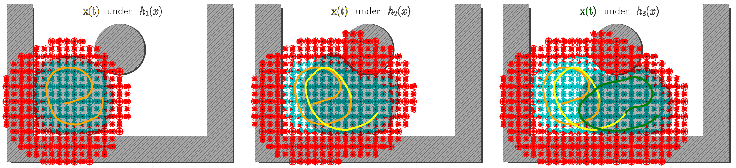
For our idealized LiDAR sensor, we define a circular scan radius of $1.1$ (depicted in red in Fig. 4) around the position $q$ of the system. Because all states outside of the scan radius could potentially be obstacles, the incrementally learned CBF must keep the system within the scan radius while avoiding detected obstacles. Our local CBFs $h_{i}(x)$ and thus also the incremental CBF $H(x)$ accomplish this requirement, while satisfying input constraints, see Figs. 2, LABEL:, and 3.

In contrast, candidate CBFs constructed from sensor scans without incorporating dynamics may not be valid and fail to satisfy safety constraints. To illustrate this point, we consider signed distance functions (SDFs), which have been used as candidate CBFs in the past, see e.g.  [7]. Fig. 4 shows that an SDF cannot provide safety for this system, even with unbounded actuation ($u_{\text{max}}=\infty)$, because the gradient of an SDF to obstacles $l(x)$ is always orthogonal to the vector field of the Dubins car (since $\partial l/\partial\theta=0$). Though high-order CBFs can be used to resolve this incompatibility, we are able to control the system with a simpler, first-order CBF.

The dynamics of the planar system are:

with $\delta:=0.33$ and initial condition $x(0)=(0,0)$. We consider the input constraints $|u|\leq u_{\textrm{max}}=1$. The environment consists of two vertically-aligned circular obstacles and four walls (Fig. 5). The scan radius of the LiDAR sensor is $1$.

Here, we compare our incremental CBF $H(x)$ with a CBF that is trained in a single-shot on all the data that was used to incrementally train $H(x)$. We find that not only do we match the performance of such a single-shot CBF, but our incremental CBF also performs better in this case (Fig. 5). Specifically, the zero-level set is closer to the obstacle, and larger gradients allow the system to approach a target more quickly. This is not surprising, as the maximum of continuously-differentiable CBFs is a more expressive function class than a single continuously differentiable CBF. Furthermore, incrementally learning a CBF is almost three times faster ($5.2$s total for four local CBFs vs. $14.9$s).

References

- [1] A. Robey, H. Hu, L. Lindemann, H. Zhang, D. V. Dimarogonas, S. Tu, and N. Matni, “Learning control barrier functions from expert demonstrations,” 2020.
- [2] L. Lindemann, A. Robey, L. Jiang, S. Das, S. Tu, and N. Matni, “Learning robust output control barrier functions from safe expert demonstrations,” IEEE Open Journal of Control Systems, 2024.
- [3] H. Zhao, X. Zeng, T. Chen, Z. Liu, and J. Woodcock, “Learning safe neural network controllers with barrier certificates,” Formal Aspects of Computing, vol. 33, pp. 437–455, 2021.
- [4] D. Sun, S. Jha, and C. Fan, “Learning certified control using contraction metric,” in Conference on Robot Learning. PMLR, 2021, pp. 1519–1539.
- [5] P. Glotfelter, J. Cortés, and M. Egerstedt, “Boolean composability of constraints and control synthesis for multi-robot systems via nonsmooth control barrier functions,” in 2018 IEEE Conference on Control Technology and Applications (CCTA). IEEE, 2018, pp. 897–902.
- [6] H. Wendland, “Piecewise polynomial, positive definite and compactly supported radial functions of minimal degree,” Advances in computational Mathematics, vol. 4, pp. 389–396, 1995.
- [7] K. Long, C. Qian, J. Cortés, and N. Atanasov, “Learning barrier functions with memory for robust safe navigation,” IEEE Robotics and Automation Letters, vol. 6, no. 3, pp. 4931–4938, 2021.
- [8] M. Srinivasan, A. Dabholkar, S. Coogan, and P. A. Vela, “Synthesis of control barrier functions using a supervised machine learning approach,” in 2020 IEEE/RSJ International Conference on Intelligent Robots and Systems (IROS). IEEE, 2020, pp. 7139–7145.
- [9] S. Bansal, M. Chen, S. Herbert, and C. J. Tomlin, “Hamilton-jacobi reachability: A brief overview and recent advances,” in 2017 IEEE 56th Annual Conference on Decision and Control (CDC). IEEE, 2017, pp. 2242–2253.
- [10] A. D. Ames, S. Coogan, M. Egerstedt, G. Notomista, K. Sreenath, and P. Tabuada, “Control barrier functions: Theory and applications,” 2019.
- [11] J. J. Choi, D. Lee, K. Sreenath, C. J. Tomlin, and S. L. Herbert, “Robust control barrier–value functions for safety-critical control,” in 2021 60th IEEE Conference on Decision and Control (CDC). IEEE, 2021, pp. 6814–6821.
- [12] L. Lindemann and D. V. Dimarogonas, “Control barrier functions for signal temporal logic tasks,” IEEE control systems letters, vol. 3, no. 1, pp. 96–101, 2018.
- [13] M. Black and D. Panagou, “Consolidated control barrier functions: Synthesis and online verification via adaptation under input constraints,” arXiv preprint arXiv:2304.01815, 2023.
- [14] S. Yang, M. Black, G. Fainekos, B. Hoxha, H. Okamoto, and R. Mangharam, “Safe control synthesis for hybrid systems through local control barrier functions,” arXiv preprint arXiv:2311.17201, 2023.
- [15] Z. Gao, G. Yang, and A. Prorok, “Online control barrier functions for decentralized multi-agent navigation,” in 2023 International Symposium on Multi-Robot and Multi-Agent Systems (MRS). IEEE, 2023, pp. 107–113.
- [16] W. Luo, W. Sun, and A. Kapoor, “Sample-efficient safe learning for online nonlinear control with control barrier functions,” in International Workshop on the Algorithmic Foundations of Robotics. Springer, 2022, pp. 419–435.
- [17] C. Li, Z. Zhang, A. Nesrin, Q. Liu, F. Liu, and M. Buss, “Instantaneous local control barrier function: An online learning approach for collision avoidance,” arXiv preprint arXiv:2106.05341, 2021.
- [18] A. S. Lafmejani, S. Berman, and G. Fainekos, “Nmpc-lbf: Nonlinear mpc with learned barrier function for decentralized safe navigation of multiple robots in unknown environments,” in 2022 IEEE/RSJ International Conference on Intelligent Robots and Systems (IROS). IEEE, 2022, pp. 10 297–10 303.
- [19] Y. Zhang, G. Tian, L. Wen, X. Yao, L. Zhang, Z. Bing, W. He, and A. Knoll, “Online efficient safety-critical control for mobile robots in unknown dynamic multi-obstacle environments,” arXiv preprint arXiv:2402.16449, 2024.
- [20] A. Safari and J. B. Hoagg, “Time-varying soft-maximum control barrier functions for safety in an a priori unknown environment,” arXiv preprint arXiv:2310.05261, 2023.
- [21] A. Rahimi and B. Recht, “Random features for large-scale kernel machines,” Advances in neural information processing systems, vol. 20, 2007.
- [22] L. Lindemann, H. Hu, A. Robey, H. Zhang, D. Dimarogonas, S. Tu, and N. Matni, “Learning hybrid control barrier functions from data,” in Conference on Robot Learning. PMLR, 2021, pp. 1351–1370.
- [23] J. V. Frasch, A. Gray, M. Zanon, H. J. Ferreau, S. Sager, F. Borrelli, and M. Diehl, “An auto-generated nonlinear mpc algorithm for real-time obstacle avoidance of ground vehicles,” in 2013 European Control Conference (ECC). IEEE, 2013, pp. 4136–4141.
- [24] P. T. An and N. T. Le, “Multiple shooting approach for finding approximately shortest paths for autonomous robots in unknown environments in 2d,” Journal of Combinatorial Optimization, vol. 47, no. 5, pp. 1–32, 2024.
- [25] A. Barbu and H. Mou, “The compact support neural network,” Sensors, vol. 21, no. 24, p. 8494, 2021.