Inclusion of higher-order terms in the border-collision normal form: persistence of chaos and applications to power converters.
Abstract
The dynamics near a border-collision bifurcation are approximated to leading order by a continuous, piecewise-linear map. The purpose of this paper is to consider the higher-order terms that are neglected when forming this approximation. For two-dimensional maps we establish conditions under which a chaotic attractor created in a border-collision bifurcation persists for an open interval of parameters beyond the bifurcation. We apply the results to a prototypical power converter model to prove the model exhibits robust chaos.
1 Introduction
While most engineering systems are designed to operate outside chaotic parameter regimes, in some situations the presence of chaos is advantageous. Examples include optical resonators for which additional energy can be stored when photons follow chaotic trajectories as without periodic motion they become trapped for longer times [1]. In mechanical energy harvesters the presence of chaos allows high-energy modes of operation to be stabilised with only a small control force [2]. Also, power converters, when run chaotically, have the advantage of increased electromagnetic compatibility due to broad spectral characteristics [3]. Regardless of whether or not chaos is desired, it is extremely helpful to understand when and why it occurs.
Power converters, and many other engineering systems, function by switching between different modes of operation. There is a growing understanding of the creation of chaos in such systems through use of the border-collision normal form (BCNF). This is a piecewise-linear (or more precisely, piecewise-affine) map that models the dynamics near parameter values at which a fixed point intersects a boundary between two modes of operation [4, 5]. The piecewise-linear nature of the BCNF makes it possible to prove results about chaotic attractors and their persistence, a phenomenon called robust chaos [6, 7, 8].
The BCNF is obtained using coordinate transformations to make the lowest order terms of the map as simple as possible. The map is then truncated, ignoring all terms that are nonlinear with respect to variables and parameters. As such, it is by no means clear that results for chaotic attractors in the BCNF carry over to the full nonlinear models originally being considered. In this paper we prove a persistence result showing that, under certain conditions, the existence of a chaotic attractor in the BCNF implies the existence of a chaotic attractor in the corresponding full model regardless of the nature of the nonlinear terms that have been neglected to form the BCNF. This shows that chaotic attractors created in border-collision bifurcations typically persist for an open interval of parameters beyond the bifurcation and justifies our use of the BCNF for determining when chaotic attractors are created.
In earlier work [9] we described a computational method for determining when the two-dimensional BCNF is chaotic by establishing the existence of a trapping region in phase space and a contracting-invariant expanding cone in tangent space. The trapping region guarantees the existence of an attractor, while the cone ensures it has a positive Lyapunov exponent. In this paper we use the robustness of these objects to demonstrate persistence with respect to higher-order terms. The most difficult technical issue we have to overcome is in showing that the higher-order terms do not cause orbits of the map to accumulate new symbolic itineraries that cannot be handled by the cone.
The remainder of the paper is arranged as follows. In section 2 we describe the two-dimensional BCNF and its relation to nonlinear models. We then state our persistence result in section 3. In section 4 we provide a detailed description of the geometric structure of the phase space of the BCNF that we use in section 5 to prove the persistence result. The result, together with computational methods of [9], are then applied to a model of power converters with pulse-width modulated control, section 6. We believe this verifies, for the first time, the long-standing belief from numerical simulations that chaos occurs robustly in these types of systems. Finally section 7 contains concluding remarks.
2 Border-collision bifurcations and the border-collision normal form
The study of border-collision bifurcations has a long history dating back to at least Feigin and coworkers in the context of relay control [10, 11]. The two-dimensional BCNF was introduced by Nusse and Yorke in [4] motivated by observations of anomalous behaviour in piecewise-linear economics models [12]. The BCNF has since been shown to display a remarkably rich array of dynamics, such as robust chaos [6], multi-stability [13], multi-dimensional attractors [14], and resonance regions with sausage-string structures [15, 16]. The BCNF is relevant for describing a wide-range of physical phenomena, another example being mechanical systems with stick-slip friction [17]; see [18] for a recent review.
Let be a continuous, piecewise-smooth map with variable and parameter . We are interested in the dynamics local to a border-collision bifurcation where a fixed point of collides with a switching manifold as is varied. Assuming the bifurcation occurs at single smooth switching manifold, only two pieces of the map are relevant to the local dynamics. By choosing coordinates so that the switching manifold is , we can assume has the form
| (2.1) |
where and are .
Suppose the border-collision bifurcation occurs at when . By continuity, is a fixed point of both and when :
| (2.2) |
From the map we can extract the four key values
| (2.3) |
which determine the eigenvalues associated with for the two smooth components of (2.1). We can then use these values to form the piecewise-linear map
| (2.4) |
This is the two-dimensional BCNF, except often -dependence is retained in the constant term. In the remainder of this section we explain how (2.4) can be used to describe the local dynamics of (2.1) near the border-collision bifurcation.
We first write the components of (2.1) as
| (2.5) |
where the two expressions share several coefficients due to the assumed continuity of (2.1) on . By dropping the higher-order terms we obtain the piecewise-linear map
| (2.6) |
This approximates (2.1) in the following sense: for any there exists such that if then .
The piecewise-linear map (2.6) satisfies the identity for any . For this reason the magnitude of only affects the spatial scale of the dynamics of (2.6): if is an invariant set of for some , then is an invariant set of with for all . In view of this scaling property, we can convert (2.6) to (2.4) for any . This is achieved via the change of variables
| (2.7) |
where
| (2.8) |
and is valid assuming
| (2.9) | ||||
| (2.10) |
The condition ensures (2.7) is invertible (if then (2.6) can be partly decoupled [18]). We require so that unfolds the border-collision bifurcation in a generic fashion, while ensures the left and right components of (2.6) transform to their respective components in (2.4). The case can be accommodated by simply redefining as .
The transformation (2.7) performs a similarity transform to the Jacobian matrices of the components of the map, thus it preserves their traces and determinants. For this reason the values (2.3) were used to construct (2.4) — notice how , , , and are the traces and determinants of the Jacobian matrices of the two components of (2.4).
In summary, for any map of the form (2.1) that has a border-collision bifurcation at , we can use the values (2.3) to form the BCNF (2.4). Then, if the conditions (2.9)–(2.10) are satisfied, the BCNF is affinely conjugate to the piecewise-linear approximation to (2.1) for any . Intuitively this approximation should be reasonable for sufficiently small values of . Our persistence result in the next section gives conditions under which the approximation can indeed be justified.
3 Persistence of chaotic attractors
Our main result, Theorem 3.11 below, links the existence of chaotic attractors of the piecewise-linear BCNF (2.4) to attractors of the nonlinear map (2.1) for small . To state the result we need some preliminary definitions and conditions.
Let
denote the left and right components of the BCNF, , where
Theorem 3.11 requires the assumptions
| (3.1) | ||||
| (3.2) | ||||
| (3.3) |
where the subscript in (3.3) indicates we are looking at the second component of the vector . Conditions (3.1) and (3.2) imply that is a homeomorphism, so exists and (3.3) is well-defined. Condition (3.3) ensures the backwards orbit of the origin does not enter the closed upper half-plane . In fact, the backwards orbit is constrained to the fourth quadrant of so is governed purely by and simply converges to the unique fixed point of (a repelling focus), see Fig. 1. Together conditions (3.1)–(3.3) allow us to divide phase space by the number of iterations required to cross the switching manifold
and this is achieved in section 4. Having a precise understanding of this division is critical to our proof of Theorem 3.11 presented in section 5.

To motivate the following definitions, consider the forward orbit of a point under . Suppose it maps under times, then under times. That is, , hence , assuming no iterates lie on where is non-differentiable. For orbits that go back and forth across without landing on , which includes almost all orbits in the chaotic attractors we wish to analyse, derivatives of for large can be expressed as products of matrices of the form . Consequently we can estimate Lyapunov exponents based on bounds for the values of and .
Let
denote the closed left and right half-planes.
Definition 3.1.
Given , let be the smallest for which and let be the smallest for which , if such and exist.
Now define the regions
| (3.4) | ||||
| (3.5) |
The following result shows that when an orbit crosses from right to left, it must arrive at a point in . Moreover, is exactly the set of all such points. The set admits the same characterisation for orbits crossing from left to right. The result follows immediately from the observation that and have opposite signs.
Lemma 3.1.
Suppose and . Then
Now given a set , suppose there exist numbers and such that
| (3.6) | ||||
| (3.7) | ||||
| (3.8) | ||||
| (3.9) |
That is, any point in requires at most iterations to cross , and at least iterations if its preimage lies in . The numbers and similarly bound the number of iterations required to cross from right to left.
For the given set , let
| (3.10) |
In Theorem 3.11, is be assumed to be a trapping region for , that is, , where denotes interior. Also, to ensure a positive Lyapunov exponent, we assume has a contracting-invariant, expanding cone. This is defined as follows and illustrated in Fig. 2.

Definition 3.2.
A cone is a non-empty set for which for all and . A cone is contracting-invariant for a collection of matrices if for all and . A cone is expanding for if there exists such that for all and .
Finally we state the main result. We write for the ball of radius centred at .
Theorem 3.2.
Let be a piecewise- map of the form (2.1) satisfying (2.2). Let be the corresponding map (2.4) formed by using the values (2.3). Suppose
- i)
- ii)
-
iii)
there exists a contracting-invariant, expanding cone for .
Then there exists and such that for all the map has a topological attractor with the property that for Lebesgue almost all there exists such that
| (3.11) |
Notice is chaotic in the sense of a positive Lyapunov exponent, as implied by (3.11).
4 A partition of the plane
In this section we describe the geometry of the regions of the left half-plane with different values of and regions of the right half-plane with different values of for the BCNF (2.4). The ways in which their images intersect can be used to establish conditions under which chaotic attractors exist [9]. The regions corresponding to values of were described in [19], so for these we simply state results without proof. The regions corresponding to values of can be described in a similar way; details of these calculations are provided in Appendix A.
Definition 4.1.
For each , let
| (4.1) | ||||
| (4.2) |

First consider the sets . As shown by Proposition 6.6 of [19], each is bounded by the lines , , and , Fig. 3. If the line is not vertical, let denote its slope and denote its -intercept, i.e.,
| (4.3) |
Definition 4.2.
Let be the smallest for which , with if for all .
The next result is a simple consequence of results obtained in [19]. Recall is the third quadrant (3.4).
Lemma 4.1.
Suppose . If then the sets , for , are non-empty and cover . If then for all .
For example with , as in Fig. 3, we have . Fig. 4 shows how the value of , and hence the values of for which , depends on the values of and . Between curves where and , we have if and only if . As these curves accumulate on where has repeated eigenvalues. With , and every is non-empty.

In regards to Theorem 3.11, while the values of and depend on the particular trapping region being considered, Lemma 4.1 tells us that the value of could always be as low as , while the value of cannot be more than .
Next we note that the boundaries of the intersect the -axis transversally. This is the case because each is a line intersecting the -axis at with , see Lemma 6.2 of [19]. These transversal intersections are used to argue persistence in section 5.
Lemma 4.2.
Suppose and , with , is a point on the boundary of some . Then, local to , the boundary of is a line segment that intersects transversally.
We now turn our attention to the sets . To characterise these we assume and satisfy (3.2) and (3.3). Condition (3.2) implies has the unique fixed point
| (4.4) |
which lies in the fourth quadrant. Condition (3.3) ensures that the set of for which admits a relatively simple characterisation and that the boundaries of the intersect the -axis transversally.
By an analogous argument to that for the sets , the lines , , and form the boundaries of the . However, their layout is more complicated than that of the . Fig. 3 shows a typical example.
If the line is not vertical, let denote its slope and denote its -intercept, i.e.,
| (4.5) |
If is vertical we write (in this case is the line , see Appendix A).
Definition 4.3.
Let be the smallest for which or . Let be the smallest for which .
Lemma 4.3.

Lemma 4.3 is proved in Appendix A. The values of and are determined by the values of and as indicated in Fig. 5. As we move about the -plane, the value of changes by one when we cross a curve where , and the value of changes by one when we cross a curve where . These curves accumulate on past which has real eigenvalues and condition (3.2) is no longer satisfied. In Fig. 5, condition (3.3) is satisfied above the piecewise-smooth black curve.
5 Proof of Theorem 3.11
The proof is divided into six steps.
Step 1 — Robustness of the cone.
Let be a contracting-invariant, expanding cone for of (3.10)
and let be a corresponding expansion factor as in Definition 3.2.
Here we show that is an invariant expanding cone for
a collection of matrices
that are sufficiently close to some matrix in .
Note, the expansion factor will be instead of .
We first define a function from the space of matrices to the space of subsets of as follows: given a matrix , let
By the definition of an contracting-invariant expanding cone, given we have and . The function is continuous, so if is sufficiently close to then and . That is, for all ,
| (5.1) |
To be precise, there exists such that if for some then (5.1) is satisfied for all . Furthermore, there exists such that and implies
| (5.2) |
for all and , and that any such and are invertible (which is possible because and are invertible by (3.1) and (3.2)).
Step 2 — Bounds related to .
By the definition of , , , and ,
see (3.6)–(3.9),
we have
and .
In this step we use the results of section 4 and the
fact that maps to its interior under
to control the behaviour of points inside and near .
Since is compact there exists such that
| (5.3) |
as illustrated in Fig. 6. Now consider the set . This set is contained in except has some points just above the negative -axis. By Lemma 4.2, we can assume is small enough that does not intersect any ‘other’ regions , that is . Further, by shrinking this set by a small amount, the result will be bounded away from the other regions . That is, there exists such that for all :
-
i)
for all , and
-
ii)
if for all , then .
Also, by (3.7). Thus by (5.3) we can assume is small enough that for all :
-
iii)
if for all , then .
In view of Lemma 4.4 we can assume and are small enough that analogous bounds also hold for .

Step 3 — Change of coordinates.
Here we apply the coordinate change (2.7) for converting to plus higher order terms.
For small this coordinate change represents a spatial blow-up of phase space near the origin.
Since the higher order terms are small near the origin
we are able to control the higher order terms by assuming is sufficiently small.
Here we also let be such that .
We first decompose (2.7) into the spatial blow-up
| (5.4) |
and the bounded coordinate change
| (5.5) |
Notice (5.5) is invertible because , (2.9). The coordinate change (5.5) transforms to a map
| (5.6) |
where
| (5.7) |
The higher order terms and are and . Thus given any there exists such that
| (5.8) |
and
| (5.9) |
Then, since (2.10), the spatial blow-up (5.4) converts (5.6) with to a map of the form
| (5.10) |
where and . By (5.7)–(5.9) we have
| (5.11) |
and
| (5.12) |
Further assume so that, by (5.3), is a trapping region for with any . That is a trapping region implies has a topological attractor . Then is the corresponding attractor of . Since and is a linear function of the pair , there exists such that for all .
Step 4 — Extend bounds on to the perturbed map .
In Step 2 we obtained bounds on the number of iterations
required for orbits of the BCNF to cross .
Here we show the same bounds hold for the perturbed map .
We first extend the definitions of and to . Given , let be the smallest for which and let be the smallest for which , if such and exist. In view of Lemma 3.1, we can similarly generalise and by defining
| (5.13) |
These sets are sketched in Fig. 6 and for sufficiently small they are within of and in the bounded set . Next, take small enough so that, by (5.11), and for all . For small enough , (5.11) also implies
| (5.14) |
Then by (i) and (ii) of Step 2, and analogous bounds on ,
| (5.15) |
Step 5 — Construct an induced map .
Let
as indicated in Fig. 6. In this step we introduce an induced map that provides the first return to under iterations of .
Fix . Points in map to under iterations of . Similarly, points in map to under iterations of . Consequently we can define by
| (5.16) |
where and . Let be the set of all points whose forward orbits under intersect . Then is well-defined at any . By (5.2) and (5.12),
| (5.17) |
where and are as in (5.16). Note (5.17) also relies on the bounds and provided by (5.15).
Step 6 — Bound the Lyapunov exponent.
Finally we verify (3.11).
Choose any .
We have by (5.11) because .
Then by (5.14) and (i)–(iii) of Step 2,
there exists such that .
Let .
Also let
and
(the inverse exists by the last remark in Step 1).
For each , let and let and be the corresponding and values in (5.16). Then for all we have where . For all , let . By (5.1) and (5.17) and an inductive argument on , we have and for all . Hence . Since , we have
Since the coordinate transformation is invertible, the same bound applies to with and , i.e. (3.11). Since this applies to any , where has zero Lebesgue measure, (3.11) holds for Lebesgue almost all .
6 An application to power converters
Power converters take a raw input voltage and use control strategies to produce an output that is close to a desired voltage [20, 21]. These have applications in many areas including personal electronic equipment where the voltage from a domestic electricity supplier is different from the voltage required by the device. A prototypical DC/DC power converter model described in [22, 23] is written in terms of time-dependent variables and that represent linear combinations of an internal current and voltage as
| (6.1) |
where is the Heaviside function and
| (6.2) | ||||
| (6.3) |
The function is the control signal employed by the converter. In this model time has been scaled so that the switching period is , see section 5.2 of [22] for more details. The floor function denotes the largest integer less than or equal to .
Here we fix
| (6.4) |
and vary the value of which represents input voltage and is a controllable parameter. The values (6.4) are as given in [23] except we have used a slightly larger value of so that the border-collision bifurcation produces a chaotic attractor instead of an invariant torus.

Fig. 7 shows a typical time series of (6.1). On the vertical axis we have plotted which is an affine function of the variables. The system switches from (black) to (orange) when the purple line meets the green line , and switches back to at integer times.
We now provide a stroboscopic map that captures the dynamics of (6.1). This map is given in [23] and is straight-forward to derive. Let , for , denote the solution to (6.1) at integer times. The stroboscopic map, , is
| (6.5) |
where
| (6.6) |
and
| (6.7) |
Fig. 8 shows a bifurcation diagram of (6.5). As the value of is increased, a stable fixed point undergoes a border-collision bifurcation at
| (6.8) |
Numerical simulations suggest that a chaotic attractor is created in the border-collision bifurcation. The numerically computed Lyapunov exponent remains positive until . Fig. 9(a) shows a phase portrait of the chaotic attractor.

The map (6.5) has two switching manifolds. The border-collision bifurcation occurs on the switching manifold , so for the purposes of analyzing the local dynamics associated with this bifurcation we can ignore the component of (6.6). Upon performing the affine change of variables
| (6.9) |
the map (without the component of (6.6)) takes the form (2.1). Also let
| (6.10) |
which with (2.2) is satisfied, i.e. the border-collision bifurcation occurs at when . By differentiating (6.5) and evaluating it at the border-collision bifurcation we obtain
| (6.11) |
By substituting (6.4) and (6.8) into (6.11) and rounding to four decimal places we obtain
| (6.12) |
We now show that this border-collision bifurcation satisfies the conditions of Theorem 3.11. Certainly (2.9) is satisfied; (2.10) is also satisfied due to signs choices made when constructing (6.9). Conditions (3.1)–(3.3) are satisfied with in Definition 4.2 (the eigenvalues of are complex) and and in Definition 4.3.
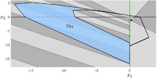
With (6.12) the BCNF has the forward invariant region shown in Fig. 10. This region was constructed using the algorithm of [9] (specifically is the union of images of a ‘recurrent’ region ). For we have
| (6.13) |
in (3.6)–(3.9). While does not map to its interior, i.e. only , by generalising the approach used in [19] we have observed numerically that can be shrunk by a small amount to produce a trapping region that necessarily satisfies (3.6)–(3.9) with the same bounds on and .
For the collection , the algorithm in [9] also produces the invariant expanding cone
where and . By Proposition 8.1 of [9], this cone can be enlarged slightly to produce a cone that is contracting-invariant and expanding.
This shows that the border-collision bifurcation of the power converter model satisfies the conditions of Theorem 3.11. We can therefore conclude that the model has a chaotic attractor for all , for some . Based on the numerically computed Lyapunov exponent shown in Fig. 8, we could possibly take . By inverting the coordinate changes required to go from the stroboscopic map to the BCNF , we were able to reproduce the attractor of with (6.12) in the coordinates of , and this shown in Fig. 9(b).
7 Discussion
The border-collision normal form has attracted a great deal of attention because it acts as a paradigm for the dynamics of general piecewise-smooth systems, and because it has a broad variety of applications. In both contexts it is important to know which features of the dynamics are particular to the piecewise-linear character of the BCNF, and which are persistent features of piecewise-smooth systems. Certainly in applications this question is fundamental to the interpretation of results.
In this paper we have established techniques that can be used to prove that a chaotic attractor observed in the BCNF persists with the addition of nonlinear terms close to a border-collision bifurcation. The techniques are sufficiently simple that the conditions can be checked in explicit examples, and we have achieved this for a prototypical power converter model. This approach appears to be quite effective because it is possible to use analytic (or simple, finite numerical calculations) to prove the existence of chaotic attractors in the BCNF, then use persistence arguments to infer the existence of chaotic attractors in the original system. This eliminates the need to compute asymptotic quantities, such as Lyapunov exponents, or to rely on a visual examination of numerically computed attractors.
For the power converter model, the chaotic attractor appears to vary continuously (with respect to Hausdorff metric) as is varied just past the border-collision bifurcation. This is why the attractor of the BCNF shown in Fig. 9(b) closely resembles that of the power converter shown in Fig. 9(a). It remains to determine general conditions that ensure continuity, perhaps by employing the result of Hoang et. al. [24], see [25].
This work feeds into a larger (and often unspoken) question about the BCNF: is it a normal form in the strict, bifurcation theory sense of the term [26]? The dynamics of a (strict) normal form is equivalent to those of the original system in some neighbourhood of parameter space and phase space. In contrast, in Theorem 3.11 the neighbourhood shrinks to a point at the bifurcation. These concepts depend on the type of equivalence being used and the result of this paper comes a step closer to showing that, with an appropriate definition of equivalence, the BCNF can indeed be a normal form in this stronger, technical sense.
Acknowledgements
The authors were supported by Marsden Fund contract MAU1809, managed by Royal Society Te Apārangi.
Appendix A Calculations for the regions
We first show how the values of and can be computed iteratively. By substituting , which represents , into
| (A.1) |
we obtain
| (A.2) |
which represents . From (A.2) we see that the slope and -intercept of are
| (A.3) |
assuming . If , then , and from (A.2) we see that is the vertical line . Further, by substituting this into (A.1) we obtain
and therefore in this case the slope and -intercept of are
| (A.4) |
To obtain starting values for the iterations, notice is the -axis, so . By substituting these into (A.4) we obtain and .
In summary, starting with and we can use (A.3) to iteratively generate and for all , using instead (A.4) for the special case .
We now prove Lemmas 4.3 and 4.4 together. This is achieved by carefully characterising the regions and here the reader may find it helpful to refer to Fig. 3.
Proof of Lemmas 4.3 and 4.4.
We first describe the backwards orbit of under . Notice and . Thus, for all , the points and lie on . They are distinct points, hence is the unique line that passes through these points. By (3.2)–(3.3),
| (A.5) |
Thus for each and any point sufficiently close to , we have by the definition of . Further, there exist points arbitrarily close to such that . Therefore
| (A.6) |
where denotes closure and denotes boundary.
Next we characterise the regions up to . By definition, consists of all for which . We have , therefore
| (A.7) |
recalling and . For each , consists of all for which . It follows that
| (A.8) |
By (A.7), is the region bounded by two rays emanating from . One ray is part of , the other ray is part of and contains the point . Then from (A.6) and (A.8), for all the region is bounded by two rays emanating from . One ray is part of , the other ray is part of and contains the point . By (A.5) and the definition of , for all , whereas .
Notice contains an infinite section of the positive -axis. The preimage of the -axis under is the -axis, thus contains an infinite section of the positive -axis. Therefore has three boundaries:
-
i)
a ray (part of emanating from ),
-
ii)
the line segment from to , and
-
iii)
the part of above .
Finally, if , then for all , is the triangle with vertices , , and . This in part relies on the observation which is a consequence of (A.3) and the definition of . For each we have because . Our precise description of the implies , and this completes the proof Lemma 4.3. Further, we have shown that the boundaries of do not coincide with an interval the -axis or have vertices on the -axis, and this completes the proof of Lemma 4.4. ∎
References
- [1] C. Liu, A. Di Falco, D. Molinari, Y. Khan, B.S. Ooi, T.F. Krauss, and A. Fratalocchi. Enhanced energy storage in chaotic optical resonators. Nature Photon., 7:473–478, 2013.
- [2] A. Kumar, S.F. Ali, and A. Arockiarajan. Enhanced energy harvesting from nonlinear oscillators via chaos control. IFAC-PapersOnLine, 49(1):35–40, 2016.
- [3] J.H.B. Deane and D.C. Hamill. Improvement of power supply EMC by chaos. Electron. Lett., 32(12):1045, 1996.
- [4] H.E. Nusse and J.A. Yorke. Border-collision bifurcations including “period two to period three” for piecewise smooth systems. Phys. D, 57:39–57, 1992.
- [5] M. di Bernardo, C.J. Budd, A.R. Champneys, and P. Kowalczyk. Piecewise-smooth Dynamical Systems. Theory and Applications. Springer-Verlag, New York, 2008.
- [6] S. Banerjee, J.A. Yorke, and C. Grebogi. Robust chaos. Phys. Rev. Lett., 80(14):3049–3052, 1998.
- [7] S. Banerjee and C. Grebogi. Border collision bifurcations in two-dimensional piecewise smooth maps. Phys. Rev. E, 59(4):4052–4061, 1999.
- [8] P. Glendinning. Robust chaos revisited. Eur. Phys. J. Special Topics, 226(9):1721–1738, 2017.
-
[9]
P. Glendinning and D.J.W. Simpson.
Chaos in the border-collision normal form: A computer-assisted
proof using induced maps and invariant expanding cones.
arXiv:2108.05999, 2021. - [10] V.A. Brousin, Yu.I. Neimark, and M.I. Feigin. On some cases of dependence of periodic motions of relay system upon parameters. Izv. Vyssh. Uch. Zav. Radiofizika, 4:785–800, 1963. In Russian.
- [11] M.I. Feigin. Doubling of the oscillation period with -bifurcations in piecewise continuous systems. Prikl. Mat. Mekh., 34(5):861–869, 1970. In Russian.
- [12] C.H. Hommes and H.E. Nusse. “Period three to period two” bifurcation for piecewise linear models. J. Economics, 54(2):157–169, 1991.
- [13] M. Dutta, H.E. Nusse, E. Ott, J.A. Yorke, and G. Yuan. Multiple attractor bifurcations: A source of unpredictability in piecewise smooth systems. Phys. Rev. Lett., 83(21):4281–4284, 1999.
- [14] P. Glendinning. Bifurcation from stable fixed point to 2D attractor in the border collision normal form. IMA J. Appl. Math., 81(4):699–710, 2016.
- [15] D.J.W. Simpson and J.D. Meiss. Shrinking point bifurcations of resonance tongues for piecewise-smooth, continuous maps. Nonlinearity, 22(5):1123–1144, 2009.
- [16] D.J.W. Simpson. The structure of mode-locking regions of piecewise-linear continuous maps: I. Nearby mode-locking regions and shrinking points. Nonlinearity, 30(1):382–444, 2017.
- [17] M. di Bernardo, P. Kowalczyk, and A. Nordmark. Sliding bifurcations: A novel mechanism for the sudden onset of chaos in dry friction oscillators. Int. J. Bifurcation Chaos, 13(10):2935–2948, 2003.
- [18] D.J.W. Simpson. Border-collision bifurcations in . SIAM Rev., 58(2):177–226, 2016.
- [19] D.J.W. Simpson. Detecting invariant expanding cones for generating word sets to identify chaos in piecewise-linear maps. Submitted., 2020.
- [20] S. Banerjee and G.C. Verghese, editors. Nonlinear Phenomena in Power Electronics. IEEE Press, New York, 2001.
- [21] C.K. Tse. Complex Behavior of Switching Power Converters. CRC Press, Boca Raton, FL, 2003.
- [22] Z.T. Zhusubaliyev and E. Mosekilde. Bifurcations and Chaos in Piecewise-Smooth Dynamical Systems. World Scientific, Singapore, 2003.
- [23] Z.T. Zhusubaliyev and E. Mosekilde. Equilibrium-torus bifurcation in nonsmooth systems. Phys. D, 237:930–936, 2008.
- [24] L.T. Hoang, E.J. Olson, and J.C. Robinson. On the continuity of global attractors. Proc. Amer. Math. Soc., 143:4389–4395, 2015.
- [25] P.A. Glendinning and D.J.W. Simpson. Robust chaos and the continuity of attractors. Trans. Math. Appl., 4(1):tnaa002, 2020.
- [26] Yu.A. Kuznetsov. Elements of Bifurcation Theory., volume 112 of Appl. Math. Sci. Springer-Verlag, New York, 3rd edition, 2004.