In the Danger Zone: U-Net Driven Quantile Regression can Predict High-risk SARS-CoV-2 Regions via Pollutant Particulate Matter and Satellite Imagery
Abstract
Since the outbreak of COVID-19 policy makers have been relying upon non-pharmacological interventions to control the outbreak. With air pollution as a potential transmission vector there is need to include it in intervention strategies. We propose a U-net driven quantile regression model to predict air pollution based on easily obtainable satellite imagery. We demonstrate that our approach can reconstruct concentrations on ground-truth data and predict reasonable values with their spatial distribution, even for locations where pollution data is unavailable. Such predictions of characteristics could crucially advise public policy strategies geared to reduce the transmission of and lethality of COVID-19.
1 Introduction
Since the outbreak of the Severe Acute Respiratory Syndrome Corona Virus 2 (SARS-CoV-2), popularly referred to as COVID-19, many questions have been asked around the disease. Of particular interest are the questions of transmission methods, and characteristics that identify vulnerable populations. Studies into these properties are made more complex by the lack of information around the behavior of the virus, E.g. the percent of cases that are asymptomatic. However, as indicated by the inclusion in the CDC’s vulnerable Population index, asthma and chronic lung disease seem to be a major factor in the severity of the cases. For example, in (Conticini et al., 2020) the connections between the lethality rate in Lombardy and Emilia Romagna, areas with high level of atmospheric pollution, are explored. In particular, the paper studies the correlation between pollution, which is a known instigator of chronic lung disease even in young and other wise healthy subjects, and the lethality of SARS-CoV-2. A similar result for the lethality in the United States (Wu et al., 2020) using county level fatality rate, and county level long term air pollution, shows that, after adjusting for other known factors, that there is a strong correlation between the concentration of particulate matter micrometers or less in diameter, or , and the county level lethality. Specifically, a 1 increase in corresponds to an increase in the fatality rate.
However, as observed in (Coccia, 2020), there is also a correlation between particulate matter () air pollution and the number of reported cases. This suggests that pollution-to-human may serve as another transmission dynamic for SARS-CoV-2. These two results suggest a two factor vulnerability to SARS-CoV-2 caused by increased particulate matter in the air: On one hand it increases the likelihood of having a more sever reaction to infection, and the other it serves a transmission vector.

Traditionally, concentration data can be obtained from ground sensors and measurement stations. However, the spatial resolution of these measurements is greatly limited by the sparsity of sensor networks. Thus, detailed pollution maps have been developed that integrate heterogeneous data sources (see e.g. van Donkelaar et al. (2019)), to create a database of estimated monthly pollutant concentrations over several countries. This data was used by Wu et al. (2020) linking concentrations to COVID-19 mortality rates. Although this historical data helped establish this causality relationship, up-to-date/live pollution information is still needed to monitor pollutant .
By knowing where pollution is we can better understand the impacts of social segregation policy on subpopulations in order to e.g. allocate medical funds to the most vulnerable populaces. The health needs for a population often require very granular data about their circumstances, and air pollution is one such measure that is only sporadically known in poorer areas and thus is insufficiently represented in modeling the health situation. In order to properly control COVID-19 hotspots there is a need to predict the spread and intensity of COVID-19. While contact tracing and non-pharmacological interventions (NPIs) have shown value, there is mounting evidence that there are other transmission vectors, including via pollution particles, as discussed earlier. Therefore there is mounting need to understand local pollution dynamics in order to correctly deal with the pandemic. In order to properly understand the effectiveness of a given NPI it is essential we understand the main transmission vectors. It is, therefore, vital we gain understanding of the strength of air pollution as a transmission vector in order to understand and design NPIs efficiently.
The goal of the present work is to model air pollution concentrations using readily available satellite imagery. The aim is to aid in any planning for efficacious COVID-19 geared strategies. The paper is organized as follows: Sec. 2 introduces the proposed U-net model, Sec. 3 presents the data, Sec. 4 describes the experiments and results, and finally Sec. 5 provides a summary and outlook.
2 U-net model for pollutant particulate matter
We build upon the well known U-net architecture (Ronneberger et al., 2015) to predict dense (per-pixel) concentrations from multispectral satellite imagery. Since its introduction in 2015, the U-net has been successfully applied to various semantic segmentation tasks, E.g. in medical imaging (Dong et al., 2017) and astronomy(Akeret et al., 2017). The U-net consists of two symmetrical parts. The encoder path downsamples the original image into meaningful features by means of convolutional filters and pooling operations, whereas the upsampling path aims at decoding these features into a full-sized output map using transposed convolution operations, driven by an appropriate loss function. Moreover, upsampling layers are augmented with feature maps from the downsampling path at the corresponding resolution, to provide more context information. The original U-net was meant for classification and featured a softmax layer after the top-level upsampling layer’s output, trained using a cross-entropy objective with discrete ground-truth labels. Yet the U-net has also been used for dense regression by removing the softmax layer and optimizing the squared difference between the upsampled output and a continuous target variable (Yao et al., 2018; Payer et al., 2016).
It is well known that least squares regression estimates the conditional mean of the response variable given the predictors, and is therefore sensitive to outliers. Alternatively, Quantile regression (Koenker, 2005) is more robust to outliers. Let denote a set of predictor variable vectors and matching continuous response variables sampled from their respective distributions . Let indicate the prediction function parameterized by , and let refer to the quantile level. In this work, we consider losses of the form:
| (1) |
In the above, denotes the indicator function for event , whereas the term is the check function (Koenker, 2005). To better quantify the approximated distribution, we learn 3 quantiles simultaneously, which allows us to obtain both a point-wise estimate from the median and a confidence interval for the value. We cast the aggregate loss function as a linear combination of partial terms with coefficients , in a simple multi-task learning setting (Gong et al., 2019):
| (2) |
To mirror the structure of the loss function, the U-net architecture was extended to include a separate sequence of convolutional filters at the top level of the upsampling path per quantile loss term (see Fig. 1). One disadvantage of using the loss (Eq. 1) is the fact that the check function is not differentiable at zero. Moreover, the derivative is piece-wise constant on . This might pose a challenge to gradient-based optimization schemes (E.g. back propagation in neural networks) because the gradient norm does not get smaller as the optimization converges to a local minimum. To alleviate that, some approximations of the check function have been proposed. The Huber loss (Hastie et al., 2001) combines quadratic behavior within a neighborhood of 0 with linear behavior on . This can be used to approximate . Recently, Gupta et al. (2020) introduced an asymmetric version of the Huber loss:
| (3) |

This loss function is differentiable everywhere. The parameters control both the slope of the linear functions on their respective sides of the real axis, and the locations where the function starts to show quadratic behavior. We propose to approximate with , where is a parameter which controls the location of the change from linear to quadratic characteristics. See Fig. 2 for a comparison of loss functions.
3 Data
In order to address this problem, we use satellite imagery as a source of predictor variables, and approximate concentrations published by van Donkelaar et al. (2019) for the time period of 2000-2018 in the role of ground-truth.
Satellite data. Our work used Landsat 8 satellite imagery published by the United States Geological Survey (Lan, 2016). Landsat 8 is the latest in a series of Earth observation missions containing a total of spectral bands, ranging in wavelengths from to , with spatial resolution between to depending on the band.
Pollution data. We downloaded monthly concentration maps for North America from (Don, ). Readily available, these maps contain degrees per pixel and use a standard WGS84 coordinate reference system. We used the data made available immediately after Landsat 8 mission launched, namely from March 2013 to December 2018.
Preprocessing. The Landsat imagery was first reprojected to the WGS84 coordinate system, and downsampled to the ground-truth resolution of degrees (the panchromatic band was dropped). To match the temporal resolution of the ground-truth, we computed per-band average images grouped by month of acquisition. Next, we derived a per-pixel mask of regions within the image covered by cirrus clouds and hence not suitable for analysis, based on the estimated cloud cover percentage (Foga et al., 2017). Finally, we combined the cloud cover mask with the data availability mask from the ground-truth maps. Also, pixels corresponding to the top and bottom of ground-truth values were masked out as outliers. All input imagery bands were normalized to the interval individually per band.
4 Experiments
We selected an initial number Landsat images, spanning March 2013 to December 2018, of major cities from representative regions of the United States (see Fig. 3, green boxes) and preprocessed them as described in Sec. 3. Next, we defined our ground-truth data as these images paired with corresponding images from which we use an 80:20 random split to create training/testing set of 106:27 images. A U-net based on adapting the implementation by Akeret et al. (2017) was trained using an ADAM optimized over epochs with minibatch size of and internal iterations, with the following parameterization: dropout ratio was , learning rate , regression quantiles . For the Huber loss function (3), all aggregates (2) contributed in equal proportion and the parameter controlling the function shape was .

4.1: Sanity check with ground-truth. The network converged to a state which produced a mean absolute error of between predicted and ground-truth values on the training set (see Fig. 4). The median width of the predicted confidence intervals (upper bound - lower bound) for training data was , and of ground-truth values fell into the predicted interval. The number of ground-truth values above the lower bound and below the upper bound was respectively and . This demonstrates that the model was able to approximate the and quantiles well, and also to provide quality point-estimates. Correspondingly, our approach can predict pollution maps that match the structure and approximate concentrations of ground-truth reconstructions. See Fig. 5 for some examples.
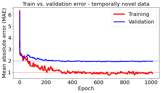

4.2: Generalizability to temporally novel data. To assess the ability of our model to generalize in the temporal domain, we utilized previously unseen images that overlapped with the training set spatially but not temporally. The test set contained images from of the cities. The mean absolute validation error followed the same trend as Exp. 4.1 with GT training data, however it converged to about (see Fig. 4). The performance of the predicted confidence intervals degraded to 40% of contained ground-truth values, whereas the median interval width remained low at . This indicates a degree of overfitting, however the predicted concentrations are still within reasonable distance of the ground-truth.
4.3: Cities with similar pollution profile. We selected new images at additional locations within the United States, showing visually similar distributions of ground-truth within the Landsat image frames to the original training cities, in order to evaluate the performance of predicting the concentrations at locations unseen during training. The obtained mean absolute error was , and the predicted confidence intervals contained of ground-truth values. This shows that it is harder to generalize in the spatial than in the temporal domain.
4.4: Before and after SARS-CoV-2-induced lock-down. The goal of the fourth experiment is to verify that our model can predict expected concentration trends at time points before and after the government mandated lock-down in March 2020 intended to hinder the spread of SARS-CoV-2 (which consequently e.g. drastically reduced industrial emissions). We applied the U-net learned in Exp. 4.3 to satellite images of Los Angeles, CA from 2018, 2019, and early 2020. The results, shown in Fig. 6, illustrate that the U-net was able to learn concentrations consistent with world events at the time. Namely, the pollution is inferred to be notably higher before the lock-down than after the lock-down, shown by the considerable shift of the predicted distribution’s quantile between October 2019 and April 2020 – the quantile shifted from to , respectively. Additionally, our approach was able to successfully isolate regions in LA that are the most densely populated by predicting higher pollutant values. This suggests that our approach can generalize to new data and reliably predict pollutant concentrations and their spatial structure, which informs on the presence and lethality of SARS-CoV-2.

5 Discussion
SARS-CoV-2 lethality has been concretely linked to the concentration of pollutant particulate matter, where a slight increase in can drastically enhance the morbidity rate. We have proposed a means of learning the structure, spatial distribution, and physical concentration of pollutant particulate matter based solely on global satellite imagery and monthly values from the years 2013-2018. Our approach proposes a U-net convolutional network with quantile regression loss to learn dense per-pixel prediction maps. We have demonstrated not only that our approach can successfully reconstruct concentrations with low error, but it can also generalize to completely unseen locations for which pollutant data is not available. As pollution has been shown to be a main vector of SARS-CoV-2 transmission, this ability to identify regions where it may be particularly transmissible and lethal can provide critical advice to implementable public health strategies, such as the ability to monitor, understand, and design NPIs efficiently.
Given that our approach passes several sanity checks by demonstrating that its concentration predictions reflect ground-truth values/measurements, it would follow that it can make meaningful predictions for locations for which there has never been recordings of the particulate matter (only satellite imagery available). Additionally, although we currently do not have rigorous methodology to quantify what makes satellite imagery of different cities ‘similar’, we could address this e.g. with dependence tests such as kernel two-sample tests (Gretton et al., 2012). Also, data from multiple satellites could be included to provide greater temporal resolution, such as from the Sentinel-2 mission (Drusch et al., 2012). With larger satellite datasets we can expect an increase in the accuracy of our predictions.
References
- (1) PM2.5 concentrations published by Aaron van Donkelaar. ftp://stetson.phys.dal.ca/Aaron/V4NA02.MAPLE/ASCII/Monthly/PM25/. Accessed: 2020-06-06.
- Lan (2016) Landsat—Earth observation satellites. Technical report, Reston, VA, 2016. Report.
- Akeret et al. (2017) Akeret, J., Chang, C., Lucchi, A., and Refregier, A. Radio frequency interference mitigation using deep convolutional neural networks. Astronomy and Computing, 18:35–39, 2017.
- Coccia (2020) Coccia, M. Two mechanisms for accelerated diffusion of COVID-19 outbreaks in regions with high intensity of population and polluting industrialization: the air pollution-to-human and human-to-human transmission dynamics. medRxiv, 2020.
- Conticini et al. (2020) Conticini, E., Frediani, B., and Caro, D. Can atmospheric pollution be considered a co-factor in extremely high level of SARS-CoV-2 lethality in Northern Italy? Environ. Pollut., 261:114465, Jun 2020.
- Dong et al. (2017) Dong, H., Yang, G., Liu, F., Mo, Y., and Guo, Y. Automatic Brain Tumor Detection and Segmentation Using U-Net Based Fully Convolutional Networks. In Valdés Hernández, M. and González-Castro, V. (eds.), Medical Image Understanding and Analysis, pp. 506–517, Cham, 2017. Springer International Publishing. ISBN 978-3-319-60964-5.
- Drusch et al. (2012) Drusch, M., Del Bello, U., Carlier, S., Colin, O., Fernandez, V., Gascon, F., Hoersch, B., Isola, C., Laberinti, P., Martimort, P., Meygret, A., Spoto, F., Sy, O., Marchese, F., and Bargellini, P. Sentinel-2: Esa’s optical high-resolution mission for gmes operational services. Remote Sensing of Environment, 120:25 – 36, 2012. ISSN 0034-4257. doi: https://doi.org/10.1016/j.rse.2011.11.026. URL http://www.sciencedirect.com/science/article/pii/S0034425712000636. The Sentinel Missions - New Opportunities for Science.
- Foga et al. (2017) Foga, S., Scaramuzza, P., Guo, S., Zhu, Z., Dilley, R., Beckman, T., Schmidt, G., Dwyer, J., Hughes, M., and Laue, B. Cloud detection algorithm comparison and validation for operational landsat data products. Remote Sensing of Environment, 194:379–390, 2017.
- Gong et al. (2019) Gong, T., Lee, T., Stephenson, C., Renduchintala, V., Padhy, S., Ndirango, A., Keskin, G., and Elibol, O. H. A Comparison of Loss Weighting Strategies for Multi task Learning in Deep Neural Networks. IEEE Access, 7:141627–141632, 2019.
- Gretton et al. (2012) Gretton, A., Borgwardt, K., Rasch, M., Schoelkopf, B., and Smola, A. A kernel two-sample test. JMLR, 13:723–773, 2012.
- Gupta et al. (2020) Gupta, D., Hazarika, B. B., and Berlin, M. Robust regularized extreme learning machine with asymmetric Huber loss function. Neural Computing and Applications, Jan 2020. ISSN 1433-3058.
- Hastie et al. (2001) Hastie, T., Tibshirani, R., and Friedman, J. The Elements of Statistical Learning. Springer Series in Statistics. Springer New York Inc., New York, NY, USA, 2001.
- Koenker (2005) Koenker, R. Quantile Regression. Econometric Society Monographs. Cambridge University Press, 2005.
- Payer et al. (2016) Payer, C., Štern, D., Bischof, H., and Urschler, M. Regressing Heatmaps for Multiple Landmark Localization using CNNs. In Ourselin, S., Joskowicz, L., Sabuncu, M. R., Unal, G., and Wells, W. (eds.), Medical Image Computing and Computer-Assisted Intervention – MICCAI 2016, pp. 230–238, Cham, 2016. Springer International Publishing. ISBN 978-3-319-46723-8.
- Ronneberger et al. (2015) Ronneberger, O., Fischer, P., and Brox, T. U-Net: Convolutional Networks for Biomedical Image Segmentation. CoRR, abs/1505.04597, 2015.
- van Donkelaar et al. (2019) van Donkelaar, A., Martin, R. V., Li, C., and Burnett, R. T. Regional Estimates of Chemical Composition of Fine Particulate Matter Using a Combined Geoscience-Statistical Method with Information from Satellites, Models, and Monitors. Environmental Science & Technology, 53(5):2595–2611, 2019.
- Wu et al. (2020) Wu, X., Nethery, R. C., Sabath, B. M., Braun, D., and Dominici, F. Exposure to air pollution and COVID-19 mortality in the United States: A nationwide cross-sectional study. medRxiv, 2020.
- Yao et al. (2018) Yao, W., Zeng, Z., Lian, C., and Tang, H. Pixel-wise regression using U-Net and its application on pansharpening. Neurocomputing, 312:364 – 371, 2018. ISSN 0925-2312.