This paper was converted on www.awesomepapers.org from LaTeX by an anonymous user.
Want to know more? Visit the Converter page.

Improving the Knowledge Gradient Algorithm

Le Yang
Department of Systems Engineering
City University of Hong Kong
[email protected]
&Siyang Gao
Department of Systems Engineering
City University of Hong Kong
[email protected]
&Chin Pang Ho
School of Data Science
City University of Hong Kong
[email protected]
Abstract

The knowledge gradient (KG) algorithm is a popular policy for the best arm identification (BAI) problem. It is built on the simple idea of always choosing the measurement that yields the greatest expected one-step improvement in the estimate of the best mean of the arms. In this research, we show that this policy has limitations, causing the algorithm not asymptotically optimal. We next provide a remedy for it, by following the manner of one-step look ahead of KG, but instead choosing the measurement that yields the greatest one-step improvement in the probability of selecting the best arm. The new policy is called improved knowledge gradient (iKG). iKG can be shown to be asymptotically optimal. In addition, we show that compared to KG, it is easier to extend iKG to variant problems of BAI, with the ϵ\epsilon-good arm identification and feasible arm identification as two examples. The superior performances of iKG on these problems are further demonstrated using numerical examples.

1 Introduction

The best arm identification (BAI) is a sequential decision problem where in each stage, the agent pulls one out of kk given arms and observes a noisy sample of the chosen arm. At the end of the sampling stage, the agent needs to select the arm that is believed to be the best according to the samples. In this research, we let the best arm be the one with the largest mean. BAI is a useful abstraction of issues faced in many practical settings berry1978modified ; gilotte2018offline and has been widely studied in the machine learning community even2006action ; audibert2010best . Since in practical problems, the target arm(s) (to be identified) is not necessarily the best arm, some variant models of BAI have also been proposed in the literature, e.g., top-mm arm identification bubeck2013multiple ; xiao2018simulation , Pareto front identification auer2016pareto , ϵ\epsilon-good arm identification mason2020finding , feasible arm identification gao2016efficient ; katz2018feasible , etc.

In this research, we focus on the fixed-budget BAI, in which the total number of samples (budget) is fixed and known by the agent. The goal is to correctly identify the best arm when the budget is used up. To solve this problem, many methods have been proposed, e.g., successive rejects (SR) audibert2010best , expected improvements (EI) chick2010sequential , top-two sampling qin2017improving ; russo2020simple , knowledge gradient (KG) ryzhov2010robustness ; li2022finite , optimal computing budget allocation (OCBA)chen2000simulation ; gao2017new ; li2023convergence , etc. Among these methods, KG has been prevailing. It was first proposed in gupta1994bayesian and further analyzed in frazier2008knowledge ; frazier2009knowledge . It is built on the simple idea of always pulling the arm that yields the greatest expected one-step improvement in the estimate of the best mean of the arms. This improvement measure is analytical, making the algorithm easily implementable. KG often offers reasonable empirical performances and has been successfully applied in a number of real applications schoppe2010wind ; negoescu2011knowledge .

However, we observe that this definition of KG has limitations, causing the algorithm not asymptotically optimal. Here by not being asymptotically optimal, we mean that the KG algorithm is not rate optimal, in the sense that the probability of the best arm being falsely selected based on the posterior means of the kk arms does not converge to zero at the fastest possible rate. This is resulted from KG allocating too few samples to the best arm and excessive samples to the remaining arms. Note that Frazier et al. frazier2008knowledge claimed that KG is “asymptotically optimal”, but in their context, “asymptotically optimal” is consistent, i.e., all the arms will be infinitely sampled as the round nn\rightarrow\infty, so that the best arm will be correctly selected eventually. This is a relatively weak result for BAI algorithms (the simple equal allocation is also consistent). In this paper, asymptotically optimal refers to rate optimal.

Contributions. We propose a new policy that can overcome this limitation of KG. The new policy follows the manner of one-step look ahead of KG, but pulls the arm that yields the greatest one-step improvement in the probability of selecting the best arm. We call it improved knowledge gradient (iKG) and show that it is asymptotically optimal. This policy is originated from the thought of looking at whether the best arm has been selected at the end of sampling, instead of looking at the extent that the mean of the selected arm has been maximized. Although both ways can identify the best arm, it turns out that the algorithms developed from them are significantly different in the rates of posterior convergence. Another advantage of iKG over KG is that iKG is more general and can be more easily extended to variant problems of BAI. We use ϵ\epsilon-good arm identification and feasible arm identification as examples, develop algorithms for them using the idea of iKG and establish asymptotic optimality for the algorithms.

This paper is conceptually similar to qin2017improving which improves the EI algorithm for BAI. However, for EI, sampling ratios of any two arms in the non-best set are already asymptotically optimal. One only needs to introduce a parameter β\beta to balance the probabilities of sampling the best arm and the non-best set without changing the sampling policy within the non-best set to further improve EI. For KG, sampling ratios are not asymptotically optimal for any two out of the kk arms. It requires a fundamental change on the sampling policy that influences the sampling rates of all the arms to improve KG. Moreover, the improved rate of posterior convergence of EI in qin2017improving still depends on β\beta which is not necessarily optimal, while we can show that this rate of iKG is optimal.

2 Knowledge Gradient and its Limitations

In this section, we review KG and discuss its limitations. Suppose there are kk arms in BAI. In each round tt, the agent chooses any arm ii to pull and obtains a noisy sample Xt+1,iX_{t+1,i}. After nn rounds, the agent needs to select an arm that he/she believes to be the best. Under the framework of the KG algorithm, Xt+1,iX_{t+1,i}’s are assumed to be independent across different rounds tt and arms ii and following the normal distribution 𝒩(μi,σi2)\mathcal{N}(\mu_{i},\sigma_{i}^{2}) with unknown means μi\mu_{i} and known variances σi2\sigma_{i}^{2}. The best arm is assumed to be unique. Without loss of generality, let μ1>μ2μk\mu_{\langle 1\rangle}>\mu_{\langle 2\rangle}\geq\ldots\geq\mu_{\langle k\rangle}, where i\langle i\rangle indicates the arm with ii-th largest mean.

The KG algorithm can be derived from a dynamic programming (DP) formulation of BAI. The state space 𝕊\mathbb{S} consists of all the possible posterior means and variances of the arms, denoted as 𝕊k×(0,)k\mathbb{S}\triangleq\mathbb{R}^{k}\times(0,\infty)^{k}. State StS_{t} in round tt can be written as St=(μt,1,μt,2,,μt,k,σt,12,σt,22,,σt,k2)S_{t}=(\mu_{t,1},\mu_{t,2},\ldots,\mu_{t,k},\sigma_{t,1}^{2},\sigma_{t,2}^{2},\ldots,\sigma_{t,k}^{2})^{\top}. In the Bayesian model, the unknown mean μi\mu_{i} is treated as random and let θi\theta_{i} be the random variable following its posterior distribution. We adopt normal distribution priors 𝒩(μ0,i,σ0,i2)\mathcal{N}(\mu_{0,i},\sigma_{0,i}^{2}). With samples of the arms, we can compute their posterior distributions, which are still normal 𝒩(μt,i,σt,i2)\mathcal{N}(\mu_{t,i},\sigma_{t,i}^{2}) in round tt by conjugacy. The posterior mean and variance of arm ii are

μt+1,i={σt,i2μt,i+σi2Xt+1,iσt,i2+σi2if It=i,μt,iif Iti,andσt+1,i2={1σt,i2+σi2if It=i,σt,i2if Iti.\mu_{t+1,i}=\left\{\begin{aligned} &\frac{\sigma_{t,i}^{-2}\mu_{t,i}+\sigma_{i}^{-2}X_{t+1,i}}{\sigma_{t,i}^{-2}+\sigma_{i}^{-2}}&{\mbox{if~{}}I_{t}=i},\\ &\mu_{t,i}&{\mbox{if~{}}I_{t}\neq i},\end{aligned}\right.\quad\mbox{and}\quad\sigma_{t+1,i}^{2}=\left\{\begin{aligned} &\frac{1}{\sigma_{t,i}^{-2}+\sigma_{i}^{-2}}&{\mbox{if~{}}I_{t}=i},\\ &\sigma_{t,i}^{2}&{\mbox{if~{}}I_{t}\neq i}.\end{aligned}\right. (1)

In this paper, we adopt a non-informative prior for each arm i𝔸i\in\mathbb{A}, i.e., μ0,i=0\mu_{0,i}=0 and σ0,i=\sigma_{0,i}=\infty. Denote the action space as 𝔸{1,2,,k}\mathbb{A}\triangleq\{1,2,\ldots,k\} and transition function as 𝒯𝕊×𝔸×𝕊𝕊\mathcal{T}\triangleq\mathbb{S}\times\mathbb{A}\times\mathbb{S}\rightarrow\mathbb{S}. Suppose θt,i\theta_{t,i} is a random variable following the posterior distribution 𝒩(μt,i,σi2)\mathcal{N}(\mu_{t,i},\sigma_{i}^{2}) of arm ii. Then, the state transition can be written as St+1=𝒯(St,i,θt,i)S_{t+1}=\mathcal{T}(S_{t},i,\theta_{t,i}). Let π\pi be the sampling policy that guides the agent to pull arm ItI_{t} in round tt and Π\Pi be the set of sampling policies π=(I0,I1,,In1)\pi=(I_{0},I_{1},\ldots,I_{n-1}) adapted to the filtration I0,X1,I0,,It1,Xt,It1I_{0},X_{1,I_{0}},\ldots,I_{t-1},X_{t,I_{t-1}}. After nn rounds, the estimated best arm InI_{n}^{*} is selected and a terminal reward vn(Sn)v_{n}(S_{n}) is received. We can write our objective as

supπΠ𝔼πvn(Sn).\sup_{\pi\in\Pi}\mathbb{E}_{\pi}v_{n}(S_{n}). (2)

The DP principle implies that the value function in round 0t<n0\leq t<n can be computed recursively by

vt(S)maxi𝔸𝔼[vt+1(𝒯(S,i,θt,i))],S𝕊.v_{t}(S)\triangleq\max_{i\in\mathbb{A}}\mathbb{E}[v_{t+1}(\mathcal{T}(S,i,\theta_{t,i}))],\quad S\in\mathbb{S}.

We define the Q-factors as

Qt(S,i)𝔼[vt+1(𝒯(S,i,θt,i))],S𝕊,Q_{t}(S,i)\triangleq\mathbb{E}[v_{t+1}(\mathcal{T}(S,i,\theta_{t,i}))],\quad S\in\mathbb{S},

and the DP principle tells us that any policy satisfying

It(S)argmaxi𝔸Qt(S,i),S𝕊I_{t}(S)\in\operatorname*{argmax}_{i\in\mathbb{A}}Q_{t}(S,i),\quad S\in\mathbb{S}

is optimal. However, the optimal policy is basically intractable unless for problems with very small scales, known as the “curse of dimensionality”.

On the other hand, note that except the terminal reward vn(Sn)v_{n}(S_{n}), this problem has no rewards in the other rounds, so we can restructure vn(Sn)v_{n}(S_{n}) as a telescoping sequence

vn(Sn)=[vn(Sn)vn(Sn1)]++[vn(St+1)vn(St)]+vn(St).v_{n}(S_{n})=[v_{n}(S_{n})-v_{n}(S_{n-1})]+\ldots+[v_{n}(S_{t+1})-v_{n}(S_{t})]+v_{n}(S_{t}).

Thus, vn(Sn)v_{n}(S_{n}) can be treated as the cumulation of multiple one-step improvements vn(Sl)vn(Sl1)v_{n}(S_{l})-v_{n}(S_{l-1}), l=t+1,,nl=t+1,\ldots,n. A class of one-step look ahead algorithms iteratively pull the arm that maximizes the expectation of the one-step improvement on the value function

𝔼[vn(𝒯(St,i,θt,i))vn(St)].\mathbb{E}[v_{n}(\mathcal{T}(S_{t},i,\theta_{t,i}))-v_{n}(S_{t})]. (3)

These algorithms are not optimal in general unless there is only one round left, i.e., n=t+1n=t+1.

The KG algorithm falls in this class. It sets the terminal reward as vn(Sn)=μInv_{n}(S_{n})=\mu_{I_{n}^{*}}. With this reward, the one-step improvement in (3) becomes

KGt,i=𝔼[max{𝒯(μt,i,i,θt,i),maxiiμt,i}maxi𝔸μt,i],\text{KG}_{t,i}=\mathbb{E}[\max\{\mathcal{T}(\mu_{t,i},i,\theta_{t,i}),\max_{i^{\prime}\neq i}\mu_{t,i^{\prime}}\}-\max_{i\in\mathbb{A}}\mu_{t,i}],

and in each round, the KG algorithm pulls the arm It(St)argmaxi𝔸KGt,iI_{t}(S_{t})\in\operatorname*{argmax}_{i\in\mathbb{A}}\text{KG}_{t,i}.

Input: k2k\geq 2, nn
1 Collect n0n_{0} samples for each arm ii;
2 while t<nt<n do
3       Compute KGt,i and set It=argmaxi𝔸I_{t}=\operatorname*{argmax}_{i\in\mathbb{A}}KGt,i;
4       Play ItI_{t};
5       Update μt+1,i\mu_{t+1,i} and σt+1,i\sigma_{t+1,i};
6      
Output: InI_{n}^{*}
Algorithm 1 KG Algorithm

We next characterize for the KG algorithm the rate of posterior convergence of 1{In=I}1-\mathbb{P}\{I_{n}^{*}=I^{*}\}, the probability that the best arm is falsely selected.

Proposition 1.

Let ci=(μ1μi)/σi(μ1μ2)/σ2c_{\langle i\rangle}=\frac{(\mu_{\langle 1\rangle}-\mu_{\langle i\rangle})/\sigma_{\langle i\rangle}}{(\mu_{\langle 1\rangle}-\mu_{\langle 2\rangle})/\sigma_{\langle 2\rangle}}, i=2,,ki=2,...,k. For the KG algorithm,

limn1nlog(1{In=I})=ΓKG,\lim_{n\rightarrow\infty}-\frac{1}{n}\log(1-\mathbb{P}\{I_{n}^{*}=I^{*}\})=\Gamma^{\text{KG}},

where

ΓKG=mini1((μiμ1)22((i1σ2/ci+σ1)σ1+ciσi2(i11/ci+σ1/σ2))).\Gamma^{\text{KG}}=\min_{i\neq 1}\bigg{(}\frac{(\mu_{\langle i\rangle}-\mu_{\langle 1\rangle})^{2}}{2((\sum_{i\neq 1}\sigma_{\langle 2\rangle}/c_{\langle i\rangle}+\sigma_{\langle 1\rangle})\sigma_{\langle 1\rangle}+c_{\langle i\rangle}\sigma_{\langle i\rangle}^{2}(\sum_{i\neq 1}1/c_{\langle i\rangle}+\sigma_{\langle 1\rangle}/\sigma_{\langle 2\rangle}))}\bigg{)}.

We observe that ΓKG\Gamma^{\text{KG}} is not optimal. To make this point, Proposition 2 gives an example that ΓKG\Gamma^{\text{KG}} is no better than this rate of the TTEI algorithm qin2017improving when the parameter β\beta (probability of sampling the best arm) of TTEI is set to some suboptimal value.

Proposition 2.

For the TTEI algorithm qin2017improving , the rate of posterior convergence of 1{In=I}1-\mathbb{P}\{I_{n}^{*}=I^{*}\} exists and is denoted as ΓTTEI\Gamma^{\text{TTEI}}. Let its probability of sampling the best arm β=(σ2/σ1i11/ci+1)1\beta=(\sigma_{\langle 2\rangle}/\sigma_{\langle 1\rangle}\sum_{i\neq 1}1/c_{\langle i\rangle}+1)^{-1}. We have ΓKGΓTTEI\Gamma^{\text{KG}}\leq\Gamma^{\text{TTEI}}.

According to the proof of Proposition 2, there are configurations of the BAI problem leading to ΓKG<ΓTTEI\Gamma^{\text{KG}}<\Gamma^{\text{TTEI}}, i.e., ΓKG\Gamma^{\text{KG}} is not optimal. In fact, with β=(σ2/σ1i11/ci+1)1\beta=(\sigma_{\langle 2\rangle}/\sigma_{\langle 1\rangle}\sum_{i\neq 1}1/c_{\langle i\rangle}+1)^{-1}, ΓKG=ΓTTEI\Gamma^{\text{KG}}=\Gamma^{\text{TTEI}} is achieved only in some special cases, e.g., when k=2k=2.

3 Improved Knowledge Gradient

In this section, we propose an improved knowledge gradient (iKG) algorithm. We still follow the manner of one-step look ahead of KG, but set the terminal reward of problem (2) as vn(Sn)=𝟏{In=I}v_{n}(S_{n})=\mathbf{1}\{I_{n}^{*}=I^{*}\}. That is, for the goal of identifying the best arm, we reward the selected arm by a 0-1 quantity showing whether this arm is the best arm, instead of the mean of this arm (as in KG).

In this case, 𝔼[vn(Sn)]={In=I}\mathbb{E}[v_{n}(S_{n})]=\mathbb{P}\{I_{n}^{*}=I^{*}\}, where

{In=I}={iIn(θIn>θi)}=1{iIn(θi>θIn)}.\begin{split}\mathbb{P}\{I_{n}^{*}=I^{*}\}&=\mathbb{P}\bigg{\{}\bigcap\limits_{i\neq I_{n}^{*}}(\theta_{I_{n}^{*}}>\theta_{i})\bigg{\}}=1-\mathbb{P}\bigg{\{}\bigcup\limits_{i\neq I_{n}^{*}}(\theta_{i}>\theta_{I_{n}^{*}})\bigg{\}}.\end{split} (4)

However, the probability {iIn(θi>θIn)}\mathbb{P}\bigg{\{}\bigcup\limits_{i\neq I_{n}^{*}}(\theta_{i}>\theta_{I_{n}^{*}})\bigg{\}} in (4) does not have an analytical expression. To facilitate the algorithm implementation and analysis, we adopt an approximation to it using the Bonferroni inequality galambos1977bonferroni :

{iIn(θi>θIn)}iIn(θi>θIn),\mathbb{P}\bigg{\{}\bigcup\limits_{i\neq I_{n}^{*}}(\theta_{i}>\theta_{I_{n}^{*}})\bigg{\}}\leq\sum_{i\neq I_{n}^{*}}\mathbb{P}(\theta_{i}>\theta_{I_{n}^{*}}),

and 𝔼[vn(Sn)]\mathbb{E}[v_{n}(S_{n})] can be approximately computed as

𝔼[vn(Sn)]1iIn(θi>θIn)=1iInexp((μn,iμn,In)22(σn,i2+σn,In2)).\mathbb{E}[v_{n}(S_{n})]\approx 1-\sum_{i\neq I_{n}^{*}}\mathbb{P}(\theta_{i}>\theta_{I_{n}^{*}})=1-\sum_{i\neq I_{n}^{*}}\exp\Bigg{(}{-\frac{(\mu_{n,i}-\mu_{n,I_{n}^{*}})^{2}}{2(\sigma_{n,i}^{2}+\sigma_{n,I_{n}^{*}}^{2})}}\Bigg{)}. (5)

Note that the Bonferroni inequality has been adopted as an approximation of the probability of correct selection in the literature for development of BAI algorithms chen2000simulation . For our purpose, we can show that the use of this approximation still makes the resulting algorithm asymptotically optimal and empirically superior.

Input: k2k\geq 2, nn
1 Collect n0n_{0} samples for each arm ii;
2 while t<nt<n do
3       Compute iKGt,i and set It=argmaxi𝔸I_{t}=\operatorname*{argmax}_{i\in\mathbb{A}}iKGt,i;
4       Play ItI_{t};
5       Update μt+1,i\mu_{t+1,i}, σt+1,i\sigma_{t+1,i} and It+1I_{t+1}^{*};
6      
Output: InI_{n}^{*}
Algorithm 2 iKG Algorithm

Let iKGt,i be the one-step improvement in (3) with ItI_{t}^{*} treated as unchanged after one more sample and 𝔼[vn(Sn)]\mathbb{E}[v_{n}(S_{n})] approximated by (5). We have the following proposition to compute iKGt,i. The iKG algorithm pulls the arm with the largest iKGt,i in each round.

Proposition 3.

With the definition of iKGt,i above, we have

iKGt,i={exp((μt,iμt,It)22(σt,i2+σt,It2))exp((μt,iμt,It)22(σt+1,i2+σt,It2+σi2(σt+1,i2/σi2)2)),if iIt,iItexp((μt,iμt,It)22(σt,i2+σt,It2))iItexp((μt,iμt,It)22(σt,i2+σt+1,It2+σIt2(σt+1,It2/σIt2)2)),if i=It.\text{iKG}_{t,i}=\left\{\begin{aligned} &\exp\Bigg{(}{-\frac{(\mu_{t,i}-\mu_{t,I_{t}^{*}})^{2}}{2(\sigma_{t,i}^{2}+\sigma_{t,I_{t}^{*}}^{2})}}\Bigg{)}-\exp\Bigg{(}{-\frac{(\mu_{t,i}-\mu_{t,I_{t}^{*}})^{2}}{2(\sigma_{t+1,i}^{2}+\sigma_{t,I_{t}^{*}}^{2}+\sigma_{i}^{2}(\sigma_{t+1,i}^{2}/\sigma_{i}^{2})^{2})}}\Bigg{)},&{\mbox{if~{}}i\neq I_{t}^{*}},\\ &\sum\limits_{i^{\prime}\neq I_{t}^{*}}\exp\Bigg{(}{-\frac{(\mu_{t,i^{\prime}}-\mu_{t,I_{t}^{*}})^{2}}{2(\sigma_{t,i^{\prime}}^{2}+\sigma_{t,I_{t}^{*}}^{2})}}\Bigg{)}-\sum\limits_{i^{\prime}\neq I_{t}^{*}}\exp\Bigg{(}{-\frac{(\mu_{t,i^{\prime}}-\mu_{t,I_{t}^{*}})^{2}}{2(\sigma_{t,i^{\prime}}^{2}+\sigma_{t+1,I_{t}^{*}}^{2}+\sigma_{I_{t}^{*}}^{2}(\sigma_{t+1,I_{t}^{*}}^{2}/\sigma_{I_{t}^{*}}^{2})^{2})}}\Bigg{)},&{\mbox{if~{}}i=I_{t}^{*}}.\end{aligned}\right. (6)

Both KG and iKG are greedy algorithms that look at the improvement only one-step ahead. The essential difference between them is on the reward they use for the event of best arm identification. For KG, it is the mean of the arm selected, while for iKG, it is a 0-1 quantity showing whether the best arm is selected. It is interesting to note that the choice between these two rewards has been discussed in the control community for optimization of complex systems, known as cardinal optimization (similar to KG) vs. ordinal optimization (similar to iKG) ho1992ordinal , with the discussion result in line with this research, indicating that ordinal optimization has advantages over cardinal optimization in the convergence rates of the optimization algorithms ho1999explanation .

Theorem 1.

For the iKG algorithm, limn1nlog(1{In=I})=ΓiKG\lim_{n\rightarrow\infty}-\frac{1}{n}\log(1-\mathbb{P}\{I_{n}^{*}=I^{*}\})=\Gamma^{\text{iKG}}, where

ΓiKG=(μiμ1)22(σi2/wi+σ12/w1),\Gamma^{\text{iKG}}=\frac{(\mu_{\langle i\rangle}-\mu_{\langle 1\rangle})^{2}}{2(\sigma_{\langle i\rangle}^{2}/w_{\langle i\rangle}+\sigma_{\langle 1\rangle}^{2}/w_{\langle 1\rangle})}, (7)

and wiw_{i} is the sampling rate of arm ii satisfying

i=1kwi=1,w12σ12=i=2kwi2σi2 and (μiμ1)22(σi2/wi+σ12/w1)=(μiμ1)22(σi2/wi+σ12/w1),ii1.\begin{split}\sum\limits_{i=1}^{k}w_{i}=1,\quad\frac{w_{\langle 1\rangle}^{2}}{\sigma_{\langle 1\rangle}^{2}}=\sum_{i=2}^{k}\frac{w_{\langle i\rangle}^{2}}{\sigma_{\langle i\rangle}^{2}}\quad\mbox{ and }\quad\frac{(\mu_{\langle i\rangle}-\mu_{\langle 1\rangle})^{2}}{2(\sigma_{\langle i\rangle}^{2}/w_{\langle i\rangle}+\sigma_{\langle 1\rangle}^{2}/w_{\langle 1\rangle})}=\frac{(\mu_{\langle i^{\prime}\rangle}-\mu_{\langle 1\rangle})^{2}}{2(\sigma_{\langle i^{\prime}\rangle}^{2}/w_{\langle i^{\prime}\rangle}+\sigma_{\langle 1\rangle}^{2}/w_{\langle 1\rangle})},\ \ i\neq i^{\prime}\neq 1.\end{split} (8)

In addition, for any BAI algorithms,

lim supn1nlog(1{In=I})ΓiKG.\limsup_{n\rightarrow\infty}-\frac{1}{n}\log(1-\mathbb{P}\{I_{n}^{*}=I^{*}\})\leq\Gamma^{\text{iKG}}.

Theorem 1 shows that the rate of posterior convergence ΓiKG\Gamma^{\text{iKG}} of the iKG algorithm is the fastest possible. We still use TTEI as an example. This theorem indicates that ΓTTEIΓiKG\Gamma^{\text{TTEI}}\leq\Gamma^{\text{iKG}} for any β(0,1)\beta\in(0,1) and the equality holds only when β\beta is set to β\beta^{*}, where β\beta^{*} is the optimal value of β\beta and is typically unknown.

4 Variant Problems of BAI

Another advantage of iKG over KG is that iKG is more general, in the sense that it can be easily extended to solve variant problems of BAI. In the variants, the target arms to be identified are not the single best arm, but no matter how the target arms are defined, one can always look at the event that whether these arms are correctly identified at the end of sampling and investigate the probability of this event to develop iKG and the algorithm. In contrast, it is difficult to extend KG to identify arms that cannot be found through optimizing means of these (and/or other) arms. In this section, we extend iKG to two BAI variants: ϵ\epsilon-good arm identification mason2020finding and feasible arm identification katz2018feasible . We develop algorithms for them and establish their asymptotic optimality. Note that in these two variant problems, the target arms need to be found by comparing their means with some fixed values. In such cases, the idea of KG is not straightforward.

4.1 ϵ\epsilon-Good Arm Identification

We follow the notation in Sections 2 and 3. For the kk arms, suppose μ1μ2μk\mu_{\langle 1\rangle}\geq\mu_{\langle 2\rangle}\geq\ldots\geq\mu_{\langle k\rangle}. Given ϵ>0\epsilon>0, the ϵ\epsilon-good arm identification problem aims to find all the arms ii with μi>μ1ϵ\mu_{\langle i\rangle}>\mu_{\langle 1\rangle}-\epsilon, i.e., all the arms whose means are close enough to the best (ϵ\epsilon-good). Assume that no arms have means lying on μ1ϵ\mu_{\langle 1\rangle}-\epsilon. Denote the set of ϵ\epsilon-good arms as GϵG^{\epsilon} and the estimated set of ϵ\epsilon-good arms after nn rounds as GnϵG_{n}^{\epsilon}. We set the terminal reward vn(Sn)=𝟏{Gnϵ=Gϵ}v_{n}(S_{n})=\mathbf{1}\{G_{n}^{\epsilon}=G^{\epsilon}\}, i.e., whether the set GϵG^{\epsilon} is correctly selected. Then, 𝔼[vn(Sn)]={Gnϵ=Gϵ}\mathbb{E}[v_{n}(S_{n})]=\mathbb{P}\{G_{n}^{\epsilon}=G^{\epsilon}\}, where

{Gnϵ=Gϵ}={iGnϵ(θi>maxi𝔸θiϵ)i𝔸Gnϵ(θi<maxi𝔸θiϵ)}=1{iGnϵ(θi<maxi𝔸θiϵ)i𝔸Gnϵ(θi>maxi𝔸θiϵ)}.\begin{split}\mathbb{P}\{G_{n}^{\epsilon}=G^{\epsilon}\}&=\mathbb{P}\bigg{\{}\bigcap\limits_{i\in G_{n}^{\epsilon}}(\theta_{i}>\max_{i^{{}^{\prime}}\in\mathbb{A}}\theta_{i^{{}^{\prime}}}-\epsilon)\cap\bigcap\limits_{i\in\mathbb{A}\setminus G_{n}^{\epsilon}}(\theta_{i}<\max_{i^{{}^{\prime}}\in\mathbb{A}}\theta_{i^{{}^{\prime}}}-\epsilon)\bigg{\}}\\ &=1-\mathbb{P}\bigg{\{}\bigcup\limits_{i\in G_{n}^{\epsilon}}(\theta_{i}<\max_{i^{{}^{\prime}}\in\mathbb{A}}\theta_{i^{{}^{\prime}}}-\epsilon)\cup\bigcup\limits_{i\in\mathbb{A}\setminus G_{n}^{\epsilon}}(\theta_{i}>\max_{i^{{}^{\prime}}\in\mathbb{A}}\theta_{i^{{}^{\prime}}}-\epsilon)\bigg{\}}.\end{split}

Again, applying the Bonferroni inequality,

{Gnϵ=Gϵ}1iGnϵ(θi<maxi𝔸θiϵ)i𝔸Gnϵ(θi>maxi𝔸θiϵ).\mathbb{P}\{G_{n}^{\epsilon}=G^{\epsilon}\}\geq 1-\sum\limits_{i\in G_{n}^{\epsilon}}\mathbb{P}(\theta_{i}<\max_{i^{{}^{\prime}}\in\mathbb{A}}\theta_{i^{{}^{\prime}}}-\epsilon)-\sum\limits_{i\in\mathbb{A}\setminus G_{n}^{\epsilon}}\mathbb{P}(\theta_{i}>\max_{i^{{}^{\prime}}\in\mathbb{A}}\theta_{i^{{}^{\prime}}}-\epsilon). (9)

Let iKGϵt,i{}_{t,i}^{\epsilon} be the one-step improvement in (3) with ItI_{t}^{*} treated as unchanged after one more sample and 𝔼[vn(Sn)]\mathbb{E}[v_{n}(S_{n})] approximated by the right-hand side of (9). We have the following proposition to compute iKGϵt,i{}_{t,i}^{\epsilon} .

Proposition 4.

With the definition of iKGϵt,i{}_{t,i}^{\epsilon} above, we have

iKGt,iϵ={exp((μt,iμt,It+ϵ)22(σt,i2+σt,It2))exp((μt,iμt,It+ϵ)22(σt+1,i2+σt,It2+σi2(σt+1,i2/σi2)2)),if iIt,iItexp((μt,iμt,It+ϵ)22(σt,i2+σt,It2))iItexp((μt,iμt,It+ϵ)22(σt,i2+σt+1,It2+σIt2(σt+1,It2/σIt2)2)),if i=It.\text{iKG}_{t,i}^{\epsilon}=\left\{\begin{aligned} &\exp\Bigg{(}{-\frac{(\mu_{t,i}-\mu_{t,I_{t}^{*}}+\epsilon)^{2}}{2(\sigma_{t,i}^{2}+\sigma_{t,I_{t}^{*}}^{2})}}\Bigg{)}-\exp\Bigg{(}{-\frac{(\mu_{t,i}-\mu_{t,I_{t}^{*}}+\epsilon)^{2}}{2(\sigma_{t+1,i}^{2}+\sigma_{t,I_{t}^{*}}^{2}+\sigma_{i}^{2}(\sigma_{t+1,i}^{2}/\sigma_{i}^{2})^{2})}}\Bigg{)},&{\mbox{if~{}}i\neq I_{t}^{*}},\\ &\sum\limits_{i^{\prime}\neq I_{t}^{*}}\exp\Bigg{(}{-\frac{(\mu_{t,i^{\prime}}-\mu_{t,I_{t}^{*}}+\epsilon)^{2}}{2(\sigma_{t,i^{\prime}}^{2}+\sigma_{t,I_{t}^{*}}^{2})}}\Bigg{)}-\sum\limits_{i^{\prime}\neq I_{t}^{*}}\exp\Bigg{(}{-\frac{(\mu_{t,i^{\prime}}-\mu_{t,I_{t}^{*}}+\epsilon)^{2}}{2(\sigma_{t,i^{\prime}}^{2}+\sigma_{t+1,I_{t}^{*}}^{2}+\sigma_{I_{t}^{*}}^{2}(\sigma_{t+1,I_{t}^{*}}^{2}/\sigma_{I_{t}^{*}}^{2})^{2})}}\Bigg{)},&{\mbox{if~{}}i=I_{t}^{*}}.\end{aligned}\right. (10)
Input: k2k\geq 2, nn
1 Collect n0n_{0} samples for each arm ii;
2 while t<nt<n do
3       Compute iKGϵt,i{}_{t,i}^{\epsilon} and set It=argmaxi𝔸I_{t}=\operatorname*{argmax}_{i\in\mathbb{A}}iKGϵt,i{}_{t,i}^{\epsilon};
4       Play ItI_{t};
5       Update μt+1,i\mu_{t+1,i}, σt+1,i\sigma_{t+1,i} and It+1I_{t+1}^{*};
6      
Output: GnϵG_{n}^{\epsilon}
Algorithm 3 iKG-ϵ\epsilon Algorithm (ϵ\epsilon-good Arm Identification)

To identify the ϵ\epsilon-good arms, the iKG-ϵ\epsilon algorithm pulls the arm with the largest iKGϵt,i{}_{t,i}^{\epsilon} in each round. For this algorithm, we can show that the rate of posterior convergence of 1{Gnϵ=Gϵ}1-\mathbb{P}\{G_{n}^{\epsilon}=G^{\epsilon}\} is the fastest possible.

Theorem 2.

For the iKG-ϵ\epsilon algorithm, limn1nlog(1{Gnϵ=Gϵ})=Γϵ\lim_{n\rightarrow\infty}-\frac{1}{n}\log(1-\mathbb{P}\{G_{n}^{\epsilon}=G^{\epsilon}\})=\Gamma^{\epsilon}, where

Γϵ=(μiμ1+ϵ)22(σi2/wi+σ12/w1),\Gamma^{\epsilon}=\frac{(\mu_{\langle i\rangle}-\mu_{\langle 1\rangle}+\epsilon)^{2}}{2(\sigma_{\langle i\rangle}^{2}/w_{\langle i\rangle}+\sigma_{\langle 1\rangle}^{2}/w_{\langle 1\rangle})}, (11)

and wiw_{i} is the sampling rate of arm ii satisfying

i=1kwi=1,w12σ12=i=2kwi2σi2 and (μiμ1+ϵ)22(σi2/wi+σ12/w1)=(μiμ1+ϵ)22(σi2/wi+σ12/w1),ii1.\sum\limits_{i=1}^{k}w_{i}=1,\quad\frac{w_{\langle 1\rangle}^{2}}{\sigma_{\langle 1\rangle}^{2}}=\sum_{i=2}^{k}\frac{w_{\langle i\rangle}^{2}}{\sigma_{\langle i\rangle}^{2}}\quad\mbox{ and }\quad\frac{(\mu_{\langle i\rangle}-\mu_{\langle 1\rangle}+\epsilon)^{2}}{2(\sigma_{\langle i\rangle}^{2}/w_{\langle i\rangle}+\sigma_{\langle 1\rangle}^{2}/w_{\langle 1\rangle})}=\frac{(\mu_{\langle i^{\prime}\rangle}-\mu_{\langle 1\rangle}+\epsilon)^{2}}{2(\sigma_{\langle i^{\prime}\rangle}^{2}/w_{\langle i^{\prime}\rangle}+\sigma_{\langle 1\rangle}^{2}/w_{\langle 1\rangle})},\ \ i\neq i^{\prime}\neq 1. (12)

In addition, for any ϵ\epsilon-good arm identification algorithms,

lim supn1nlog(1{Gnϵ=Gϵ})Γϵ.\limsup_{n\rightarrow\infty}-\frac{1}{n}\log(1-\mathbb{P}\{G_{n}^{\epsilon}=G^{\epsilon}\})\leq\Gamma^{\epsilon}.

4.2 Feasible Arm Identification

In the feasible arm identification, samples from pulling arms ii are mm-dimensional vectors 𝑿t+1,i=[Xt+1,i1,,Xt+1,im]\bm{X}_{t+1,i}=[X_{t+1,i1},\ldots,X_{t+1,im}] instead of scalars, where each dimension of the vector corresponds to some measure of the system performance and Xt+1,ijX_{t+1,ij} is the observation associated with arm ii and measure jj. Suppose Xt+1,ijX_{t+1,ij}’s follow the normal distribution with unknown means μij\mu_{ij} and known variances σij2\sigma_{ij}^{2}. We impose constraints μijγj\mu_{ij}\leq\gamma_{j} on arms i=1,2,,ki=1,2,\ldots,k and measures j=1,2,,mj=1,2,\ldots,m. The goal of this problem is to find the set of feasible arms 𝒮1\mathcal{S}^{1}. Let the estimated set of feasible arms after nn rounds be 𝒮n1\mathcal{S}_{n}^{1} and 𝒮2=𝔸𝒮1\mathcal{S}^{2}=\mathbb{A}\setminus\mathcal{S}^{1}. We assume that Xt+1,ijX_{t+1,ij}’s are independent across different rounds tt and measures jj, and μij\mu_{ij}’s do not lie on the constraint limits γj\gamma_{j}. To facilitate the analysis, we also define for round tt the set of measures t,i1{j:μt,ijγj}\mathcal{E}_{t,i}^{1}\triangleq\{j:\mu_{t,ij}\leq\gamma_{j}\} satisfied by arm ii and the set of measures t,i2{j:μt,ij>γj}\mathcal{E}_{t,i}^{2}\triangleq\{j:\mu_{t,ij}>\gamma_{j}\} violated by arm ii.

Set the terminal reward vn(Sn)=𝟏{𝒮n1=𝒮1}v_{n}(S_{n})=\mathbf{1}\{\mathcal{S}_{n}^{1}=\mathcal{S}^{1}\}, i.e., whether the set 𝒮1\mathcal{S}^{1} is correctly selected. Then, 𝔼[vn(Sn)]={𝒮n1=𝒮1}\mathbb{E}[v_{n}(S_{n})]=\mathbb{P}\{\mathcal{S}_{n}^{1}=\mathcal{S}^{1}\}, where

{𝒮n1=𝒮1}={i𝒮n1(j=1m(θijγj))i𝒮n2(j=1m(θij>γj))}=1{i𝒮n1(j=1m(θij>γj))i𝒮n2(j=1m(θijγj))}.\begin{split}\mathbb{P}\{\mathcal{S}_{n}^{1}=\mathcal{S}^{1}\}&=\mathbb{P}\biggl{\{}\bigcap\limits_{i\in\mathcal{S}_{n}^{1}}\bigg{(}\bigcap\limits_{j=1}^{m}(\theta_{ij}\leq\gamma_{j})\bigg{)}\cap\bigcap\limits_{i\in\mathcal{S}_{n}^{2}}\bigg{(}\bigcup\limits_{j=1}^{m}(\theta_{ij}>\gamma_{j})\bigg{)}\biggr{\}}\\ &=1-\mathbb{P}\biggl{\{}\bigcup\limits_{i\in\mathcal{S}_{n}^{1}}\bigg{(}\bigcup\limits_{j=1}^{m}(\theta_{ij}>\gamma_{j})\bigg{)}\cup\bigcup\limits_{i\in\mathcal{S}_{n}^{2}}\bigg{(}\bigcap\limits_{j=1}^{m}(\theta_{ij}\leq\gamma_{j})\bigg{)}\biggr{\}}.\end{split}

Applying the Bonferroni inequality,

{𝒮n1=𝒮1}1i𝒮n1j=1m(θij>γj)i𝒮n2jt,i2(θijγj).\mathbb{P}\{\mathcal{S}_{n}^{1}=\mathcal{S}^{1}\}\geq 1-\sum_{i\in\mathcal{S}_{n}^{1}}\sum_{j=1}^{m}\mathbb{P}(\theta_{ij}>\gamma_{j})-\sum_{i\in\mathcal{S}_{n}^{2}}\prod_{j\in\mathcal{E}_{t,i}^{2}}\mathbb{P}(\theta_{ij}\leq\gamma_{j}). (13)

The inequality holds because 0<jn,i1(θijγj)10<\prod_{j\in\mathcal{E}_{n,i}^{1}}\mathbb{P}(\theta_{ij}\leq\gamma_{j})\leq 1.

Let iKGFt,i{}_{t,i}^{\text{F}} be the one-step improvement in (3) with 𝒮t1\mathcal{S}_{t}^{1}, 𝒮t2\mathcal{S}_{t}^{2} and t,i2\mathcal{E}_{t,i}^{2} treated as unchanged after one more sample and 𝔼[vn(Sn)]\mathbb{E}[v_{n}(S_{n})] approximated by the right-hand side of (13). We have the following proposition to compute iKGFt,i{}_{t,i}^{\text{F}} .

Proposition 5.

With the definition of iKGFt,i{}_{t,i}^{\text{F}} above, we have

iKGt,iF=j=1m(exp((γjμt,ij)22σt,ij2𝟏{i𝒮t1})exp((γjμt,ij)22(σt+1,ij2+σij2(σt+1,ij2/σij2)2)𝟏{i𝒮t1}))+exp(jt,i2(γjμt,ij)22σt,ij2𝟏{i𝒮t2})exp(jt,i2(γjμt,ij)22(σt+1,ij2+σij2(σt+1,ij2/σij2)2)𝟏{i𝒮t2}).\begin{split}\text{iKG}_{t,i}^{\text{F}}=&\sum_{j=1}^{m}\Bigg{(}\exp\Bigg{(}{-\frac{(\gamma_{j}-\mu_{t,ij})^{2}}{2\sigma_{t,ij}^{2}}}\mathbf{1}\{i\in\mathcal{S}_{t}^{1}\}\Bigg{)}-\exp\Bigg{(}{-\frac{(\gamma_{j}-\mu_{t,ij})^{2}}{2(\sigma_{t+1,ij}^{2}+\sigma_{ij}^{2}(\sigma_{t+1,ij}^{2}/\sigma_{ij}^{2})^{2})}}\mathbf{1}\{i\in\mathcal{S}_{t}^{1}\}\Bigg{)}\Bigg{)}\\ &+\exp\Bigg{(}{-\sum_{j\in\mathcal{E}_{t,i}^{2}}\frac{(\gamma_{j}-\mu_{t,ij})^{2}}{2\sigma_{t,ij}^{2}}}\mathbf{1}\{i\in\mathcal{S}_{t}^{2}\}\Bigg{)}-\exp\Bigg{(}{-\sum_{j\in\mathcal{E}_{t,i}^{2}}\frac{(\gamma_{j}-\mu_{t,ij})^{2}}{2(\sigma_{t+1,ij}^{2}+\sigma_{ij}^{2}(\sigma_{t+1,ij}^{2}/\sigma_{ij}^{2})^{2})}}\mathbf{1}\{i\in\mathcal{S}_{t}^{2}\}\Bigg{)}.\end{split} (14)
Input: k2k\geq 2, nn
1 Collect n0n_{0} samples for each arm ii;
2 while t<nt<n do
3       Compute iKGFt,i{}_{t,i}^{\text{F}} and set It=argmaxi𝔸I_{t}=\operatorname*{argmax}_{i\in\mathbb{A}}iKGFt,i{}_{t,i}^{\text{F}};
4       Play ItI_{t};
5       Update μt+1,i\mu_{t+1,i}, σt+1,i\sigma_{t+1,i}, 𝒮t+11\mathcal{S}_{t+1}^{1}, 𝒮t+12\mathcal{S}_{t+1}^{2}, t+1,i1\mathcal{E}_{t+1,i}^{1} and t+1,i2\mathcal{E}_{t+1,i}^{2};
6      
Output: 𝒮n1\mathcal{S}_{n}^{1}
Algorithm 4 iKG-F Algorithm (Feasible Arm Identification)

To identify the feasible arms, the iKG-F algorithm pulls the arm with the largest iKGFt,i{}_{t,i}^{\text{F}} in each round. For this algorithm, we can show that the rate of posterior convergence of 1{𝒮n1=𝒮1}1-\mathbb{P}\{\mathcal{S}_{n}^{1}=\mathcal{S}^{1}\} is also the fastest possible.

Theorem 3.

For the iKG-F algorithm, limn1nlog(1{𝒮n1=𝒮1})=ΓF\lim_{n\rightarrow\infty}-\frac{1}{n}\log(1-\mathbb{P}\{\mathcal{S}_{n}^{1}=\mathcal{S}^{1}\})=\Gamma^{\text{F}}, where

ΓF=wiminji1(γjμij)22σij2𝟏{i𝒮1}+wiji2(γjμij)22σij2𝟏{i𝒮2},\Gamma^{\text{F}}=w_{i}\min\limits_{j\in\mathcal{E}_{i}^{1}}\frac{(\gamma_{j}-\mu_{ij})^{2}}{2\sigma_{ij}^{2}}\mathbf{1}\{i\in\mathcal{S}^{1}\}+w_{i}\sum_{j\in\mathcal{E}_{i}^{2}}\frac{(\gamma_{j}-\mu_{ij})^{2}}{2\sigma_{ij}^{2}}\mathbf{1}\{i\in\mathcal{S}^{2}\}, (15)

and wiw_{i} is the sampling rate of arm ii satisfying

i=1kwi=1,wiminji1(γjμij)22σij2𝟏{i𝒮1}+wiji2(γjμij)22σij2𝟏{i𝒮2}=wiminji1(γjμij)22σij2𝟏{i𝒮1}+wiji2(γjμij)22σij2𝟏{i𝒮2},ii.\begin{split}&\sum\limits_{i=1}^{k}w_{i}=1,\quad\\ &w_{i}\min\limits_{j\in\mathcal{E}_{i}^{1}}\frac{(\gamma_{j}-\mu_{ij})^{2}}{2\sigma_{ij}^{2}}\mathbf{1}\{i\in\mathcal{S}^{1}\}+w_{i}\sum_{j\in\mathcal{E}_{i}^{2}}\frac{(\gamma_{j}-\mu_{ij})^{2}}{2\sigma_{ij}^{2}}\mathbf{1}\{i\in\mathcal{S}^{2}\}\\ &=w_{i^{\prime}}\min\limits_{j\in\mathcal{E}_{i^{\prime}}^{1}}\frac{(\gamma_{j}-\mu_{i^{\prime}j})^{2}}{2\sigma_{i^{\prime}j}^{2}}\mathbf{1}\{i^{\prime}\in\mathcal{S}^{1}\}+w_{i^{\prime}}\sum_{j\in\mathcal{E}_{i^{\prime}}^{2}}\frac{(\gamma_{j}-\mu_{i^{\prime}j})^{2}}{2\sigma_{i^{\prime}j}^{2}}\mathbf{1}\{i^{\prime}\in\mathcal{S}^{2}\},\ \ i\neq i^{\prime}.\end{split} (16)

In addition, for any feasible arm identification algorithms

lim supn1nlog(1{𝒮n1=𝒮1})ΓF.\limsup_{n\rightarrow\infty}-\frac{1}{n}\log(1-\mathbb{P}\{\mathcal{S}_{n}^{1}=\mathcal{S}^{1}\})\leq\Gamma^{\text{F}}.

5 Numerical Experiments

In this section, we show empirical performances of the iKG, iKG-ϵ\epsilon and iKG-F algorithms on synthetic and real-world examples. For the best arm identification problem, we compare iKG with the following algorithms.

  • Expected Improvement (EI) chick2010sequential . This is another common strategy for BAI. In each round, it pulls the arm offering the maximal expected improvement over the current estimate of the best mean of the arms.

  • Top-Two Expected Improvement (TTEI) qin2017improving . This is a modification of the EI algorithm by introducing a parameter β\beta to control the probabilities of sampling the best arm and the non-best set. We set the parameter β\beta in TTEI as its default value 1/21/2.

  • Knowledge Gradient. This is the algorithm under study in this research.

For the ϵ\epsilon-good arm identification problem, we compare iKG-ϵ\epsilon with the following algorithms.

  • APT Algorithm locatelli2016optimal . It is a fixed-budget algorithm for identifying the arms whose means are above a given threshold. We set the input tolerance parameter as 0.00010.0001 and the threshold as the posterior mean of the estimated best arm minus ϵ\epsilon.

  • (ST)2(\mbox{ST})^{2} Algorithm mason2020finding . It is a fixed-confidence algorithm for ϵ\epsilon-good arm identification. It pulls three arms in each round, the estimated best arm, one arm above the threshold and one arm below the threshold. We set the input tolerance parameter as 0.00010.0001 and γ=0\gamma=0.

For the feasible arm identification problem, we compare iKG-F with the following algorithms.

  • MD-UCBE Algorithm katz2018feasible . This is a fixed-budget algorithm for feasible arm identification based on the upper confidence bound. We set the input tolerance parameter as 0.00010.0001 and hyperparameter a=2536nkHa=\frac{25}{36}\frac{n-k}{H}, where HH is a constant that can be computed. Katz-Samuels and Scott katz2018feasible showed that with a=2536nkHa=\frac{25}{36}\frac{n-k}{H}, the performance of MD-UCBE is nearly optimal.

  • MD-SAR Algorithm katz2018feasible . This is a fixed-budget algorithm for feasible arm identification based on successive accepts and rejects. We set the input tolerance parameter as 0.00010.0001.

In addition, iKG, iKG-ϵ\epsilon and iKG-F will be compared with the equal allocation, where each arm is simply played with the same number of rounds. It is a naive method and is often used as a benchmark against which improvements might be measured.

The examples for testing include three synthetic examples, called Examples 1-3, and three real examples, namely the Dose-Finding Problem, Drug Selection Problem, and Caption Selection Problem. For Example 1-3 and the Dose-Finding problem, samples of the arms are two-dimensional. We call the measures of them measures 1 and 2. When the examples are tested for the best arm identification and ϵ\epsilon-good identification, only measure 1 will be used for identifying good/best arms. When the examples are tested for the feasible arm identification, both measures will be used for feasibility detection. For the Drug Selection and Caption Selection problems, samples of the arms are one-dimensional. They are tested for the best arm identification, ϵ\epsilon-good identification and feasible arm identification.

Synthetic Datasets. We consider three examples, all containing ten arms.

Example 1. The means in measure 1 of the ten arms are 0.19270.1927, 0.64380.6438, 3.05943.0594, 3.02203.0220, 1.37531.3753, 1.42151.4215, 0.91080.9108, 1.01261.0126, 0.11190.1119 and 1.88081.8808, and the means in measure 2 of the ten arms are 0.43500.4350, 0.72400.7240, 1.15661.1566, 0.85600.8560, 3.47123.4712, 0.82480.8248, 3.87973.8797,1.98191.9819, 3.24313.2431 and 1.43151.4315, all of which are uniformly generated in (0,4)(0,4). Samples of the arms are corrupted by normal noises 𝒩(0,1)\mathcal{N}(0,1). The best arm is arm 33 and 0.10.1-good arms are arms 3 and 4. For the feasible arm identification, we choose arms with means in both measures less than 22. Then the feasible arms are arms 11, 22, 66, 88 and 1010.

Example 2. We keep the setting of Example 1. Distributions of the noises for arms 1-5 are changed to 𝒩(0,4)\mathcal{N}(0,4).

Example 3. Consider functions y1(x)=0.05x2y_{1}(x)=-0.05x^{2}, y2(x)=0.06(7x)y_{2}(x)=-0.06(7-x) and y3(x)=0.06(x6)y_{3}(x)=0.06(x-6). The means in measure 1 of the ten arms are y1(x)y_{1}(x) with x=1,2,,10x=1,2,\ldots,10. The means in measure 2 of the ten arms are y2(x)y_{2}(x) with x=1,,6x=1,\ldots,6 and y3(x)y_{3}(x) with x=7,,10x=7,\ldots,10. Noises follow the normal distribution 𝒩(0,1)\mathcal{N}(0,1). The best arm is arm 11 and 0.50.5-good arms are arms 1-3. For the feasible arm identification, we choose arms with means in measure 11 greater than 0.5-0.5 and means in measure 22 less than 0. The feasible arms are arms 1-3.

Dose-Finding Problem. We use the data in genovese2013efficacy (see ACR5050 in week 1616) for treating rheumatoid arthritis by the drug secukinumab. There are four dosage levels, 2525mg, 7575mg, 150150mg, and 300300mg, and a placebo, which are treated as five arms. We develop a simulation model based on the dataset. Each arm is associated with two performance measures: the probability of the drug being effective and the probability of the drug causing infections. The means of the five arms are 𝝁𝟏=(0.151,0.259)\bm{\mu_{1}}=(0.151,0.259), 𝝁𝟐=(0.184,0.184)\bm{\mu_{2}}=(0.184,0.184), 𝝁𝟑=(0.209,0.209)\bm{\mu_{3}}=(0.209,0.209), 𝝁𝟒=(0.171,0.293)\bm{\mu_{4}}=(0.171,0.293) and 𝝁𝟓=(0.06,0.16)\bm{\mu_{5}}=(0.06,0.16). Samples of each arm are corrupted by normal noises 𝒩(0,0.25)\mathcal{N}(0,0.25). The best arm is arm 3 and the 0.03-good arms are arms 2 and 3. For the feasible arm identification, we find the arms whose probability of being effective is larger than 0.180.18 and the probability of causing infections is less than 0.250.25. The feasible arms are arms 2 and 3.

Drug Selection Problem. We consider five contraceptive alternatives based on the Drug Review Dataset (https://doi.org/10.24432/C5SK5S): Ethinyl estradiol / levonorgest, Ethinyl estradiol / norethindro, Ethinyl estradiol / norgestimat, Etonogestrel and Nexplanon, which can be treated as five arms. The dataset provides user reviews on the five drugs along with related conditions and ratings reflecting overall user satisfaction. We set the means of the five arms as μ1=5.8676\mu_{1}=5.8676, μ2=5.6469\mu_{2}=5.6469, μ3=5.8765\mu_{3}=5.8765, μ4=5.8298\mu_{4}=5.8298 and μ5=5.6332\mu_{5}=5.6332, and the variances of the five arms as σ12=3.2756\sigma_{1}^{2}=3.2756, σ22=3.4171\sigma_{2}^{2}=3.4171, σ32=3.2727\sigma_{3}^{2}=3.2727, σ42=3.3198\sigma_{4}^{2}=3.3198 and σ52=3.3251\sigma_{5}^{2}=3.3251, all calculated by the data. When this example is used for the best arm identification and ϵ\epsilon-good arm identification, the best arm (with the highest user satisfaction) and 0.003-good arm are both arm 3 (Ethinyl estradiol / norgestimat). When this example is used for feasible arm identification, we will select the drugs whose ratings are over 5.65.6, and the feasible arms are arm 11 (Ethinyl estradiol / levonorgest), arm 22 (Ethinyl estradiol / norethindro), arm 33 (Ethinyl estradiol / norgestimat), arm 44 (Etonogestrel) and arm 55 (Nexplanon).

Caption Selection Problem. We aim to select good captions based on the New Yorker Cartoon Caption Contest Dataset (https://nextml.github.io/caption-contest-data/). In the contests, each caption can be treated as an arm. The dataset provides the mean and variance of each arm, which can be used to set up our experiments. We will test contests 853 (Caption 853) and 854 (Caption 854).

In Caption 853, we randomly select ten captions as arms. We set the means of the ten arms as μ1=1.1400\mu_{1}=1.1400, μ2=1.0779\mu_{2}=1.0779, μ3=1.4160\mu_{3}=1.4160, μ4=1.0779\mu_{4}=1.0779, μ5=1.1081\mu_{5}=1.1081, μ6=1.1467\mu_{6}=1.1467, μ7=1.1333\mu_{7}=1.1333, μ8=1.1075\mu_{8}=1.1075, μ9=1.1026\mu_{9}=1.1026 and μ10=1.4900\mu_{10}=1.4900, and the variances of the arms as σ12=0.1418\sigma_{1}^{2}=0.1418, σ22=0.0991\sigma_{2}^{2}=0.0991, σ32=0.4871\sigma_{3}^{2}=0.4871, σ42=0.0728\sigma_{4}^{2}=0.0728, σ52=0.0977\sigma_{5}^{2}=0.0977, σ62=0.1809\sigma_{6}^{2}=0.1809, σ72=0.1843\sigma_{7}^{2}=0.1843, σ82=0.0970\sigma_{8}^{2}=0.0970, σ92=0.0932\sigma_{9}^{2}=0.0932 and σ102=0.4843\sigma_{10}^{2}=0.4843, which are all calculated by the data. When this example is used for the best arm identification, the best arm (with the highest funniness score) is arm 10. When this example is used for ϵ\epsilon-good arm identification, the 0.1-good arms are arms 3 and 10. When this example is used for feasible arm identification, we will select the captions whose funniness scores are over 1.4, and the feasible arms are arms 3 and 10.

Table 1: Probabilities of false selection for the tested algorithms in best arm identification problem.
Example Example 1 Example 2 Example 3 Dose-finding Drug Selection Caption 853 Caption 854
Algorithms Sample size 1000 5000 4400 18000 400 1000 1200 13000 2400 98000 1600 3000 12000 18000
BAI Equal Allocation 0.38 0.22 0.44 0.31 0.25 0.13 0.35 0.05 0.43 0.27 0.17 0.11 0.26 0.18
EI 0.36 0.21 0.40 0.28 0.28 0.22 0.46 0.21 0.46 0.37 0.14 0.12 0.26 0.23
TTEI 0.25 0.07 0.32 0.09 0.13 0.02 0.31 0.03 0.55 0.28 0.04 0.01 0.10 0.06
KG 0.29 0.14 0.32 0.13 0.14 0.03 0.40 0.03 0.44 0.28 0.04 0.01 0.11 0.05
iKG 0.21 0.03 0.23 0.03 0.09 0.01 0.29 0.01 0.38 0.23 0.02 0.00 0.07 0.04

In Caption 854, we also randomly select ten captions as arms. We set the means of the ten arms as μ1=1.1986\mu_{1}=1.1986, μ2=1.1890\mu_{2}=1.1890, μ3=1.1400\mu_{3}=1.1400, μ4=1.2621\mu_{4}=1.2621, μ5=1.1544\mu_{5}=1.1544, μ6=1.0339\mu_{6}=1.0339, μ7=1.1349\mu_{7}=1.1349, μ8=1.2786\mu_{8}=1.2786, μ9=1.1765\mu_{9}=1.1765 and μ10=1.1367\mu_{10}=1.1367, and the variances of the arms as σ12=0.1879\sigma_{1}^{2}=0.1879, σ22=0.2279\sigma_{2}^{2}=0.2279, σ32=0.1346\sigma_{3}^{2}=0.1346, σ42=0.3186\sigma_{4}^{2}=0.3186, σ52=0.1314\sigma_{5}^{2}=0.1314, σ62=0.0330\sigma_{6}^{2}=0.0330, σ72=0.1337\sigma_{7}^{2}=0.1337, σ82=0.3167\sigma_{8}^{2}=0.3167, σ92=0.1858\sigma_{9}^{2}=0.1858 and σ102=0.1478\sigma_{10}^{2}=0.1478, all calculated by the data. When this example is used for the best arm identification, the best arm is arm 8. When this example is used for ϵ\epsilon-good arm identification, the 0.05-good arms are arms 4 and 8. When this example is used for feasible arm identification, we will select the captions whose funniness scores are over 1.25, and the feasible arms are arms 4 and 8.

Table 2: Probabilities of false selection for the tested algorithms in ϵ\epsilon-good arm identification problem.
Example Example 1 Example 2 Example 3 Dose-finding Drug Selection Caption 853 Caption 854
Algorithms Sample size 1000 4000 2400 12000 400 4000 1600 6000 2600 90000 4000 10000 9400 15000
ϵ\epsilon-good Equal Allocation 0.54 0.20 0.65 0.28 0.61 0.26 0.46 0.18 0.62 0.37 0.28 0.19 0.14 0.05
APT 0.28 0.17 0.52 0.25 0.72 0.49 0.56 0.53 0.74 0.70 0.41 0.35 0.48 0.49
(ST)2(\mbox{ST})^{2} 0.29 0.07 0.35 0.11 0.51 0.06 0.38 0.17 0.64 0.34 0.21 0.10 0.12 0.04
iKG-ϵ{\epsilon} 0.17 0.03 0.29 0.00 0.48 0.03 0.34 0.06 0.60 0.27 0.10 0.02 0.11 0.03
Table 3: Probabilities of false selection for the tested algorithms in feasible arm identification problem.
Example Example 1 Example 2 Example 3 Dose-finding Drug Selection Caption 853 Caption 854
Algorithms Sample size 3400 11000 4800 14000 2200 4800 2000 4000 100000 140000 4000 10000 30600 44000
feasible arm Equal Allocation 0.34 0.26 0.33 0.23 0.22 0.14 0.22 0.18 0.03 0.03 0.36 0.29 0.18 0.07
MD-UCBE 0.27 0.16 0.33 0.26 0.05 0.01 0.20 0.17 0.06 0.06 0.32 0.15 0.06 0.04
MD-SAR 0.74 0.33 0.68 0.22 0.30 0.03 0.79 0.55 0.06 0.02 0.58 0.19 0.08 0.05
iKG-F 0.23 0.02 0.24 0.01 0.04 0.00 0.14 0.01 0.01 0.01 0.20 0.07 0.05 0.00

For the tested algorithms, probabilities of false selection (PFS) are obtained based on the average of 100 macro-replications. Tables 1-3 show the PFS of the algorithms under some fixed sample sizes (additional numerical results about the PFS and sampling rates of the tested algorithms are provided in the Supplement). The proposed iKG, iKG-ϵ\epsilon and iKG-F perform the best. For the best arm identification, EI tends to allocate too many samples to the estimated best arm, leading to insufficient exploration in the remaining arms, while KG tends to allocate too few samples to the estimated best arm, leading to excessive exploration in the remaining arms. TTEI always allocates approximately one-half budget to the estimated best arm when β=1/2\beta=1/2, leading to the budget not being the best utilized. For the ϵ\epsilon-good identification, APT and (ST)2(\mbox{ST})^{2} are inferior because the former insufficiently pulls the estimate best arm, leading to inaccurate estimates of the threshold, while the latter falls in the fixed-confidence regime that focuses on making guarantees on the probability of false selection instead of minimizing it. For the feasible arm identification, both MD-UCBE and MD-SAR allocate too many samples to the arms near the constraint limits. For the three problems, equal allocation performs the worst in general, because it does not have any efficient sampling mechanisms for identifying the target arms in these problems.

6 Conclusion

This paper studies the knowledge gradient (KG), a popular policy for the best arm identification (BAI). We observe that the KG algorithm is not asymptotically optimal, and then propose a remedy for it. The new policy follows KG’s manner of one-step look ahead, but utilizes different evidence to identify the best arm. We call it improved knowledge gradient (iKG) and show that it is asymptotically optimal. Another advantage of iKG is that it can be easily extended to variant problems of BAI. We use ϵ\epsilon-good arm identification and feasible arm identification as two examples for algorithm development and analysis. The superior performances of iKG on BAI and the two variants are further demonstrated using numerical examples.

References

  • [1] D. A. Berry. Modified two-armed bandit strategies for certain clinical trials. Journal of the American Statistical Association, 73(362):339–345, 1978.
  • [2] A. Gilotte, C. Calauzènes, T. Nedelec, A. Abraham, and S. Dollé. Offline a/b testing for recommender systems. In Proceedings of the 11th ACM International Conference on Web Search and Data Mining, pages 198–206, 2018.
  • [3] E. Even-Dar, S. Mannor, Y. Mansour, and S. Mahadevan. Action elimination and stopping conditions for the multi-armed bandit and reinforcement learning problems. Journal of Machine Learning Research, 7(6), 2006.
  • [4] J.-Y. Audibert, S. Bubeck, and R. Munos. Best arm identification in multi-armed bandits. In 23rd Conference on Learning Theory, pages 41–53, 2010.
  • [5] S. Bubeck, T. Wang, and N. Viswanathan. Multiple identifications in multi-armed bandits. In International Conference on Machine Learning, pages 258–265. PMLR, 2013.
  • [6] H. Xiao and S. Gao. Simulation budget allocation for selecting the top-m designs with input uncertainty. IEEE Transactions on Automatic Control, 63(9):3127–3134, 2018.
  • [7] P. Auer, C. K. Chiang, R. Ortner, and M. Drugan. Pareto front identification from stochastic bandit feedback. In Artificial Intelligence and Statistics, pages 939–947. PMLR, 2016.
  • [8] B. Mason, L. Jain, A. Tripathy, and R. Nowak. Finding all ϵ\epsilon-good arms in stochastic bandits. Advances in Neural Information Processing Systems, 33:20707–20718, 2020.
  • [9] S. Gao and W. Chen. Efficient feasibility determination with multiple performance measure constraints. IEEE Transactions on Automatic Control, 62(1):113–122, 2016.
  • [10] J. Katz-Samuels and C. Scott. Feasible arm identification. In International Conference on Machine Learning, pages 2535–2543. PMLR, 2018.
  • [11] S. E. Chick, J. Branke, and C. Schmidt. Sequential sampling to myopically maximize the expected value of information. INFORMS Journal on Computing, 22(1):71–80, 2010.
  • [12] C. Qin, D. Klabjan, and D. Russo. Improving the expected improvement algorithm. In Proceedings of the 31st International Conference on Neural Information Processing Systems, pages 5387–5397, 2017.
  • [13] D. Russo. Simple Bayesian algorithms for best arm identification. Operations Research, 68(6):1625–1647, 2020.
  • [14] I. O. Ryzhov, P. I. Frazier, and W. B. Powell. On the robustness of a one-period look-ahead policy in multi-armed bandit problems. Procedia Computer Science, 1(1):1635–1644, 2010.
  • [15] Y. Li and S. Gao. On the finite-time performance of the knowledge gradient algorithm. In International Conference on Machine Learning, pages 12741–12764. PMLR, 2022.
  • [16] C. H. Chen, J. Lin, E. Yücesan, and S. E. Chick. Simulation budget allocation for further enhancing the efficiency of ordinal optimization. Discrete Event Dynamic Systems, 10:251–270, 2000.
  • [17] S. Gao, W. Chen, and L. Shi. A new budget allocation framework for the expected opportunity cost. Operations Research, 65(3):787–803, 2017.
  • [18] Y. Li and S. Gao. Convergence rate analysis for optimal computing budget allocation algorithms. Automatica, 153:111042, 2023.
  • [19] S. S. Gupta and K. J. Miescke. Bayesian look ahead one stage sampling allocations for selecting the largest normal mean. Statistical Papers, 35(1):169–177, 1994.
  • [20] P. I. Frazier, W. B. Powell, and S. Dayanik. A knowledge-gradient policy for sequential information collection. SIAM Journal on Control and Optimization, 47(5):2410–2439, 2008.
  • [21] P. Frazier, W. Powell, and S. Dayanik. The knowledge-gradient policy for correlated normal beliefs. INFORMS Journal on Computing, 21(4):599–613, 2009.
  • [22] C. Schoppe. Wind and pumped-hydro power storage: Determining optimal commitment policies with knowledge gradient non-parametric estimation. B.Sc. Thesis at Princeton University, 2010.
  • [23] D. M. Negoescu, P. I. Frazier, and W. B. Powell. The knowledge-gradient algorithm for sequencing experiments in drug discovery. INFORMS Journal on Computing, 23(3):346–363, 2011.
  • [24] J. Galambos. Bonferroni inequalities. The Annals of Probability, pages 577–581, 1977.
  • [25] Y.-C. Ho, S. Sreenivas, and P. Vakili. Ordinal optimization of deds. Discrete Event Dynamic Systems, 2(1):61–88, 1992.
  • [26] Y.-C. Ho. An explanation of ordinal optimization: Soft computing for hard problems. Information Sciences, 113(3-4):169–192, 1999.
  • [27] A. Locatelli, M. Gutzeit, and A. Carpentier. An optimal algorithm for the thresholding bandit problem. In International Conference on Machine Learning, pages 1690–1698. PMLR, 2016.
  • [28] M. C. Genovese, P. Durez, H. B. Richards, J. Supronik, E. Dokoupilova, V. Mazurov, J. A. Aelion, S. H. Lee, C. E. Codding, H. Kellner, et al. Efficacy and safety of secukinumab in patients with rheumatoid arthritis: a phase ii, dose-finding, double-blind, randomised, placebo controlled study. Annals of the Rheumatic Diseases, 72(6):863–869, 2013.
  • [29] I. O. Ryzhov. On the convergence rates of expected improvement methods. Operations Research, 64(6):1515–1528, 2016.
  • [30] P. Glynn and S. Juneja. A large deviations perspective on ordinal optimization. In Proceedings of the 2004 Winter Simulation Conference, 2004., volume 1. IEEE, 2004.

Appendix A Proof of Proposition 1

To facilitate the analysis, we make the following definition. For two real-valued sequences {an}\{a_{n}\} and {bn}\{b_{n}\}, if limn1/nlog(an/bn)=0\lim_{n\rightarrow\infty}1/n\log(a_{n}/b_{n})=0, we call them logarithmically equivalent, denoted by an=˙bna_{n}\dot{=}b_{n}. We first analyze 1{In=I}1-\mathbb{P}\{I_{n}^{*}=I^{*}\}. Note that 1{In=I}={iIn(θi>θIn)}1-\mathbb{P}\{I_{n}^{*}=I^{*}\}=\mathbb{P}\bigg{\{}\bigcup\limits_{i\neq I_{n}^{*}}(\theta_{i}>\theta_{I_{n}^{*}})\bigg{\}} and we have

maxiIn(θi>θIn){iIn(θi>θIn)}(k1)maxiIn(θi>θIn).\max_{i\neq I_{n}^{*}}\mathbb{P}(\theta_{i}>\theta_{I_{n}^{*}})\leq\mathbb{P}\bigg{\{}\bigcup\limits_{i\neq I_{n}^{*}}(\theta_{i}>\theta_{I_{n}^{*}})\bigg{\}}\leq(k-1)\max_{i\neq I_{n}^{*}}\mathbb{P}(\theta_{i}>\theta_{I_{n}^{*}}).

Then 1{In=I}=˙maxiIn(θi>θIn)1-\mathbb{P}\{I_{n}^{*}=I^{*}\}\dot{=}\max_{i\neq I_{n}^{*}}\mathbb{P}(\theta_{i}>\theta_{I_{n}^{*}}). In round nn, θiθIn\theta_{i}-\theta_{I_{n}^{*}} follows 𝒩(μn,iμn,In,σn,i2+σn,In2)\mathcal{N}(\mu_{n,i}-\mu_{n,I_{n}^{*}},\sigma_{n,i}^{2}+\sigma_{n,I_{n}^{*}}^{2}). Let Φ()\Phi(\cdot) and ϕ()\phi(\cdot) be the cumulative density function and probability density function of the standard normal distribution, respectively. We have

(θi>θIn)=1Φ(μn,Inμn,iσn,i2+σn,In2).\mathbb{P}(\theta_{i}>\theta_{I_{n}^{*}})=1-\Phi\Bigg{(}\frac{\mu_{n,I_{n}^{*}}-\mu_{n,i}}{\sqrt{\sigma_{n,i}^{2}+\sigma_{n,I_{n}^{*}}^{2}}}\Bigg{)}.

Let z=μn,Inμn,iσn,i2+σn,In2z=\frac{\mu_{n,I_{n}^{*}}-\mu_{n,i}}{\sqrt{\sigma_{n,i}^{2}+\sigma_{n,I_{n}^{*}}^{2}}} and z>0z>0. By the following property of the cumulative probability function of the standard normal distribution

z(z2+1)<1Φ(z)<1zϕ(z)\frac{z}{(z^{2}+1)}<1-\Phi(z)<\frac{1}{z}\phi(z)

and μn,Inμn,i>0\mu_{n,I_{n}^{*}}-\mu_{n,i}>0, we have

(θi>θIn)=˙ϕ(μn,iμn,Inσn,i2+σn,In2)=˙exp((μn,iμn,In)22(σn,i2+σn,In2)).\mathbb{P}(\theta_{i}>\theta_{I_{n}^{*}})\dot{=}\phi\Bigg{(}\frac{\mu_{n,i}-\mu_{n,I_{n}^{*}}}{\sqrt{\sigma_{n,i}^{2}+\sigma_{n,I_{n}^{*}}^{2}}}\Bigg{)}\dot{=}\exp\Bigg{(}{-\frac{(\mu_{n,i}-\mu_{n,I_{n}^{*}})^{2}}{2(\sigma_{n,i}^{2}+\sigma_{n,I_{n}^{*}}^{2})}}\Bigg{)}. (17)

Denote Tn,iT_{n,i} as the number of samples for arm ii before round tt, i.e., Tt,il=0t1𝟏{Il=i}T_{t,i}\triangleq\sum_{l=0}^{t-1}\mathbf{1}\{I_{l}=i\}. By (1) in the main text, we have

σn,i2=1(σi2/Tn,i)1+σ0,i2.\sigma_{n,i}^{2}=\frac{1}{(\sigma_{i}^{2}/T_{n,i})^{-1}+\sigma_{0,i}^{-2}}.

Then

1{In=I}=˙maxiIn(exp((μn,iμn,In)22(σn,i2+σt,In2)))=˙exp(nminiIn(μn,iμn,In)22(σn,i2+σt,In2)).\begin{split}1-\mathbb{P}\{I_{n}^{*}=I^{*}\}&\dot{=}\max_{i\neq I_{n}^{*}}\Bigg{(}\exp\Bigg{(}{-\frac{(\mu_{n,i}-\mu_{n,I_{n}^{*}})^{2}}{2(\sigma_{n,i}^{2}+\sigma_{t,I_{n}^{*}}^{2})}}\Bigg{)}\Bigg{)}\\ &\dot{=}\exp\Bigg{(}{-n\min_{i\neq I_{n}^{*}}\frac{(\mu_{n,i}-\mu_{n,I_{n}^{*}})^{2}}{2(\sigma_{n,i}^{2}+\sigma_{t,I_{n}^{*}}^{2})}}\Bigg{)}.\end{split}

Hence

ΓKG=limn1nlog(1{In=I})=miniI(μiμI)22(σi2/wi+σI2/wI).\Gamma^{\text{KG}}=\lim_{n\rightarrow\infty}-\frac{1}{n}\log(1-\mathbb{P}\{I_{n}^{*}=I^{*}\})=\min_{i\neq I^{*}}\frac{(\mu_{i}-\mu_{I^{*}})^{2}}{2(\sigma_{i}^{2}/w_{i}+\sigma_{I^{*}}^{2}/w_{I^{*}})}. (18)

Notice that the sampling rate wiw_{i} of each arm ii of the KG algorithm has been characterized in [29], with

w1w2=σ1σ2 and wiwi=(μ1μi)/σi(μ1μi)/σi,i,i=2,3,,k and ii.\quad\frac{w_{\langle 1\rangle}}{w_{\langle 2\rangle}}=\frac{\sigma_{\langle 1\rangle}}{\sigma_{\langle 2\rangle}}\quad\mbox{ and }\quad\frac{w_{\langle i\rangle}}{w_{\langle i^{\prime}\rangle}}=\frac{(\mu_{\langle 1\rangle}-\mu_{\langle i^{\prime}\rangle})/\sigma_{\langle i^{\prime}\rangle}}{(\mu_{\langle 1\rangle}-\mu_{\langle i\rangle})/\sigma_{\langle i\rangle}},\quad i,i^{\prime}=2,3,\ldots,k\mbox{ and }i\neq i^{\prime}.

Together with i=1kwi=1\sum_{i=1}^{k}w_{i}=1, we have

w1=(σ2σ1i11ci+1)1w_{\langle 1\rangle}=\bigg{(}\frac{\sigma_{\langle 2\rangle}}{\sigma_{\langle 1\rangle}}\sum_{i\neq 1}\frac{1}{c_{\langle i\rangle}}+1\bigg{)}^{-1} (19)

and

wi=(ci(i11ci+σ1σ2))1,i=2,3,,k.w_{\langle i\rangle}=\bigg{(}c_{\langle i\rangle}\bigg{(}\sum_{i\neq 1}\frac{1}{c_{\langle i\rangle}}+\frac{\sigma_{\langle 1\rangle}}{\sigma_{\langle 2\rangle}}\bigg{)}\bigg{)}^{-1},\quad i=2,3,\ldots,k. (20)

Plugging into (18),

ΓKG=mini1((μiμ1)22((i1σ2/ci+σ1)σ1+ciσi2(i11/ci+σ1/σ2))).\Gamma^{\text{KG}}=\min_{i\neq 1}\bigg{(}\frac{(\mu_{\langle i\rangle}-\mu_{\langle 1\rangle})^{2}}{2((\sum_{i\neq 1}\sigma_{\langle 2\rangle}/c_{\langle i\rangle}+\sigma_{\langle 1\rangle})\sigma_{\langle 1\rangle}+c_{\langle i\rangle}\sigma_{\langle i\rangle}^{2}(\sum_{i\neq 1}1/c_{\langle i\rangle}+\sigma_{\langle 1\rangle}/\sigma_{\langle 2\rangle}))}\bigg{)}.

Appendix B Proof of Proposition 2

Similar to the proof of Proposition 1, we have

ΓTTEI=limn1nlog(1{In=I})=miniI(μiμI)22(σi2/wi+σI2/wI).\Gamma^{\text{TTEI}}=\lim_{n\rightarrow\infty}-\frac{1}{n}\log(1-\mathbb{P}\{I_{n}^{*}=I^{*}\})=\min_{i\neq I^{*}}\frac{(\mu_{i}-\mu_{I^{*}})^{2}}{2(\sigma_{i}^{2}/w_{i}+\sigma_{I^{*}}^{2}/w_{I^{*}})}.

Since for the TTEI algorithm,

(μiμI)22(σi2/wi+σI2/wI)=(μiμI)22(σi2/wi+σI2/wI),iiI,\frac{(\mu_{i}-\mu_{I^{*}})^{2}}{2(\sigma_{i}^{2}/w_{i}+\sigma_{I^{*}}^{2}/w_{I^{*}})}=\frac{(\mu_{i^{\prime}}-\mu_{I^{*}})^{2}}{2(\sigma_{i^{\prime}}^{2}/w_{i^{\prime}}+\sigma_{I^{*}}^{2}/w_{I^{*}})},\quad\forall i\neq i^{\prime}\neq I^{*},

we have

ΓTTEI=(μiμI)22(σi2/wi+σI2/wI)iI.\Gamma^{\text{TTEI}}=\frac{(\mu_{i}-\mu_{I^{*}})^{2}}{2(\sigma_{i}^{2}/w_{i}+\sigma_{I^{*}}^{2}/w_{I^{*}})}\quad\forall i\neq I^{*}.

According to (19), for the KG algorithm, w1=(σ2/σ1iI1/ci+1)1w_{\langle 1\rangle}=(\sigma_{\langle 2\rangle}/\sigma_{\langle 1\rangle}\sum_{i\neq I^{*}}1/c_{\langle i\rangle}+1)^{-1}. Now by setting β\beta of the TTEI algorithm to the same value, the sampling rates of the best arm from these two algorithms will be the same. According to Theorem 2 of [12], among algorithms allocating the same proportion of the samples to the best arm, ΓTTEI\Gamma^{\text{TTEI}} of the TTEI algorithm is optimal, i.e., ΓKGΓTTEI\Gamma^{\text{KG}}\leq\Gamma^{\text{TTEI}}.

Appendix C Proof of Propositions 3, 4 and 5

Propositions 3, 4 and 5 give the expressions of iKGt,i, iKGϵt,i{}_{t,i}^{\epsilon} and iKGFt,i{}_{t,i}^{\text{F}}. Below we introduce a lemma first, which will be used in the proofs of the three propositions.

Lemma 1.

If arm ii is sampled from 𝒩(μt,i,σi2)\mathcal{N}(\mu_{t,i},\sigma_{i}^{2}) in round tt, θi\theta_{i} and θi\theta_{i^{\prime}} follow 𝒩(μt,i,σt,i2)\mathcal{N}(\mu_{t,i},\sigma_{t,i}^{2}) and 𝒩(μt,i,σt,i2)\mathcal{N}(\mu_{t,i^{\prime}},\sigma_{t,i^{\prime}}^{2}) respectively. Then,

𝔼[(θi>θi)]=exp((μt,iμt,i)22(σt+1,i2+σt,i2+σi2(σt+1,i2/σi2)2)).\mathbb{E}[\mathbb{P}(\theta_{i}>\theta_{i^{\prime}})]=\exp\Bigg{(}{-\frac{(\mu_{t,i}-\mu_{t,i^{\prime}})^{2}}{2(\sigma_{t+1,i}^{2}+\sigma_{t,i^{\prime}}^{2}+\sigma_{i}^{2}(\sigma_{t+1,i}^{2}/\sigma_{i}^{2})^{2})}}\Bigg{)}.

Proof of Lemma 1:
We know that θt,i\theta_{t,i} follows 𝒩(μt,i,σi2)\mathcal{N}(\mu_{t,i},\sigma_{i}^{2}). Then by (1) of the main text, we have

μt+1,i={σt,i2μt,i+σi2θt,iσt,i2+σi2if It=i,μt,iif Iti,andσt+1,i2={1σt,i2+σi2if It=i,σt,i2if Iti.\mu_{t+1,i}=\left\{\begin{aligned} &\frac{\sigma_{t,i}^{-2}\mu_{t,i}+\sigma_{i}^{-2}\theta_{t,i}}{\sigma_{t,i}^{-2}+\sigma_{i}^{-2}}&{\mbox{if~{}}I_{t}=i},\\ &\mu_{t,i}&{\mbox{if~{}}I_{t}\neq i},\end{aligned}\right.\quad\mbox{and}\quad\sigma_{t+1,i}^{2}=\left\{\begin{aligned} &\frac{1}{\sigma_{t,i}^{-2}+\sigma_{i}^{-2}}&{\mbox{if~{}}I_{t}=i},\\ &\sigma_{t,i}^{2}&{\mbox{if~{}}I_{t}\neq i}.\end{aligned}\right.

Recall that

(θi>θIt)=˙exp((μt,iμt,It)22(σt,i2+σt,It2)).\mathbb{P}(\theta_{i}>\theta_{I_{t}^{*}})\dot{=}\exp\Bigg{(}{-\frac{(\mu_{t,i}-\mu_{t,I_{t}^{*}})^{2}}{2(\sigma_{t,i}^{2}+\sigma_{t,I_{t}^{*}}^{2})}}\Bigg{)}.

Then

𝔼[(θi>θi)]=𝔼[exp((μt+1,iμt,i)22(σt+1,i2+σt,i2))]=12πσiexp((σt,i2μt,i+σi2θt,iσt+1,i2μt,i)22(σt+1,i2+σt,i2))exp((θt,iμt,i)22σi2)𝑑θt,i=˙exp((μt,iμt,i)22(σt+1,i2+σt,i2+σi2(σt+1,i2/σi2)2)).\begin{split}\mathbb{E}[\mathbb{P}(\theta_{i}>\theta_{i^{\prime}})]&=\mathbb{E}\Bigg{[}\exp\Bigg{(}{-\frac{(\mu_{t+1,i}-\mu_{t,i^{\prime}})^{2}}{2(\sigma_{t+1,i}^{2}+\sigma_{t,i^{\prime}}^{2})}}\Bigg{)}\Bigg{]}\\ &=\frac{1}{\sqrt{2\pi\sigma_{i}}}\int_{-\infty}^{\infty}\exp\Bigg{(}{-\frac{(\frac{\sigma_{t,i}^{-2}\mu_{t,i}+\sigma_{i}^{-2}\theta_{t,i}}{\sigma_{t+1,i}^{-2}}-\mu_{t,i^{\prime}})^{2}}{2(\sigma_{t+1,i}^{2}+\sigma_{t,i^{\prime}}^{2})}}\Bigg{)}\exp\Bigg{(}-\frac{(\theta_{t,i}-\mu_{t,i^{\prime}})^{2}}{2\sigma_{i}^{2}}\Bigg{)}d\theta_{t,i}\\ &\dot{=}\exp\Bigg{(}{-\frac{(\mu_{t,i}-\mu_{t,i^{\prime}})^{2}}{2(\sigma_{t+1,i}^{2}+\sigma_{t,i^{\prime}}^{2}+\sigma_{i}^{2}(\sigma_{t+1,i}^{2}/\sigma_{i}^{2})^{2})}}\Bigg{)}.\end{split}

Proof of Proposition 3:
For the best arm identification problem, if iIti\neq I_{t}^{*},

iKGt,i=𝔼[vn(𝒯(St,i,θt,i))vn(St)]=1iiItexp((μt,iμt,It)22(σt,i2+σt,It2))exp((μt,iμt,It)22(σt+1,i2+σt,It2+σi2(σt+1,i2/σi2)2))(1iItexp((μt,iμt,It)22(σt,i2+σt,It2)))=exp((μt,iμt,It)22(σt,i2+σt,It2))exp((μt,iμt,It)22(σt+1,i2+σt,It2+σi2(σt+1,i2/σi2)2)).\begin{split}&\text{iKG}_{t,i}=\mathbb{E}[v_{n}(\mathcal{T}(S_{t},i,\theta_{t,i}))-v_{n}(S_{t})]\\ =&1-\sum_{i^{\prime}\neq i\neq I_{t}^{*}}\exp\Bigg{(}{-\frac{(\mu_{t,i^{\prime}}-\mu_{t,I_{t}^{*}})^{2}}{2(\sigma_{t,i^{\prime}}^{2}+\sigma_{t,I_{t}^{*}}^{2})}}\Bigg{)}-\exp\Bigg{(}{-\frac{(\mu_{t,i}-\mu_{t,I_{t}^{*}})^{2}}{2(\sigma_{t+1,i}^{2}+\sigma_{t,I_{t}^{*}}^{2}+\sigma_{i}^{2}(\sigma_{t+1,i}^{2}/\sigma_{i}^{2})^{2})}}\Bigg{)}\\ &-\Bigg{(}1-\sum_{i^{\prime}\neq I_{t}^{*}}\exp\Bigg{(}{-\frac{(\mu_{t,i^{\prime}}-\mu_{t,I_{t}^{*}})^{2}}{2(\sigma_{t,i^{\prime}}^{2}+\sigma_{t,I_{t}^{*}}^{2})}}\Bigg{)}\Bigg{)}\\ =&\exp\Bigg{(}{-\frac{(\mu_{t,i}-\mu_{t,I_{t}^{*}})^{2}}{2(\sigma_{t,i}^{2}+\sigma_{t,I_{t}^{*}}^{2})}}\Bigg{)}-\exp\Bigg{(}{-\frac{(\mu_{t,i}-\mu_{t,I_{t}^{*}})^{2}}{2(\sigma_{t+1,i}^{2}+\sigma_{t,I_{t}^{*}}^{2}+\sigma_{i}^{2}(\sigma_{t+1,i}^{2}/\sigma_{i}^{2})^{2})}}\Bigg{)}.\end{split}

If i=Iti=I_{t}^{*},

iKGt,i=𝔼[vn(𝒯(St,i,θt,i))vn(St)]=1iItexp((μt,iμt,It)22(σt,i2+σt+1,It2+σIt2(σt+1,It2/σIt2)2))(1iItexp((μt,iμt,It)22(σt,i2+σt,It2)))=iItexp((μt,iμt,It)22(σt,i2+σt,It2))iItexp((μt,iμt,It)22(σt,i2+σt+1,It2+σIt2(σt+1,It2/σIt2)2)).\begin{split}&\text{iKG}_{t,i}=\mathbb{E}[v_{n}(\mathcal{T}(S_{t},i,\theta_{t,i}))-v_{n}(S_{t})]\\ =&1-\sum\limits_{i^{\prime}\neq I_{t}^{*}}\exp\Bigg{(}{-\frac{(\mu_{t,i^{\prime}}-\mu_{t,I_{t}^{*}})^{2}}{2(\sigma_{t,i^{\prime}}^{2}+\sigma_{t+1,I_{t}^{*}}^{2}+\sigma_{I_{t}^{*}}^{2}(\sigma_{t+1,I_{t}^{*}}^{2}/\sigma_{I_{t}^{*}}^{2})^{2})}}\Bigg{)}-\Bigg{(}1-\sum_{i^{\prime}\neq I_{t}^{*}}\exp\Bigg{(}{-\frac{(\mu_{t,i^{\prime}}-\mu_{t,I_{t}^{*}})^{2}}{2(\sigma_{t,i^{\prime}}^{2}+\sigma_{t,I_{t}^{*}}^{2})}}\Bigg{)}\Bigg{)}\\ =&\sum\limits_{i^{\prime}\neq I_{t}^{*}}\exp\Bigg{(}{-\frac{(\mu_{t,i^{\prime}}-\mu_{t,I_{t}^{*}})^{2}}{2(\sigma_{t,i^{\prime}}^{2}+\sigma_{t,I_{t}^{*}}^{2})}}\Bigg{)}-\sum\limits_{i^{\prime}\neq I_{t}^{*}}\exp\Bigg{(}{-\frac{(\mu_{t,i^{\prime}}-\mu_{t,I_{t}^{*}})^{2}}{2(\sigma_{t,i^{\prime}}^{2}+\sigma_{t+1,I_{t}^{*}}^{2}+\sigma_{I_{t}^{*}}^{2}(\sigma_{t+1,I_{t}^{*}}^{2}/\sigma_{I_{t}^{*}}^{2})^{2})}}\Bigg{)}.\end{split}

Proof of Proposition 4:
We explore the expression of 𝔼[vn(Sn)]\mathbb{E}[v_{n}(S_{n})] in the ϵ\epsilon-good arm identification problem first. We know that

𝔼[vn(Sn)]=1iGnϵ(θi<maxi𝔸θiϵ)i𝔸Gnϵ(θi>maxi𝔸θiϵ).\mathbb{E}[v_{n}(S_{n})]=1-\sum\limits_{i\in G_{n}^{\epsilon}}\mathbb{P}(\theta_{i}<\max_{i^{{}^{\prime}}\in\mathbb{A}}\theta_{i^{{}^{\prime}}}-\epsilon)-\sum\limits_{i\in\mathbb{A}\setminus G_{n}^{\epsilon}}\mathbb{P}(\theta_{i}>\max_{i^{{}^{\prime}}\in\mathbb{A}}\theta_{i^{{}^{\prime}}}-\epsilon).

Note that in round nn, θiθIn+ϵ\theta_{i}-\theta_{I_{n}^{*}}+\epsilon follows 𝒩(μn,iμn,In+ϵ,σn,i2+σn,In2)\mathcal{N}(\mu_{n,i}-\mu_{n,I_{n}^{*}}+\epsilon,\sigma_{n,i}^{2}+\sigma_{n,I_{n}^{*}}^{2}). Similarly as in the proof of Proposition 1, we can know that if iGnϵi\in G_{n}^{\epsilon}

(θi<maxi𝔸θiϵ)=˙exp((μn,iμn,In+ϵ)22(σn,i2+σn,In2)),\mathbb{P}(\theta_{i}<\max_{i^{{}^{\prime}}\in\mathbb{A}}\theta_{i^{{}^{\prime}}}-\epsilon)\dot{=}\exp\Bigg{(}{-\frac{(\mu_{n,i}-\mu_{n,I_{n}^{*}}+\epsilon)^{2}}{2(\sigma_{n,i}^{2}+\sigma_{n,I_{n}^{*}}^{2})}}\Bigg{)},

and if i𝔸Gnϵi\in\mathbb{A}\setminus G_{n}^{\epsilon}

(θi>maxi𝔸θiϵ)=˙exp((μn,iμn,In+ϵ)22(σn,i2+σn,In2)).\mathbb{P}(\theta_{i}>\max_{i^{{}^{\prime}}\in\mathbb{A}}\theta_{i^{{}^{\prime}}}-\epsilon)\dot{=}\exp\Bigg{(}{-\frac{(\mu_{n,i}-\mu_{n,I_{n}^{*}}+\epsilon)^{2}}{2(\sigma_{n,i}^{2}+\sigma_{n,I_{n}^{*}}^{2})}}\Bigg{)}.

Then

𝔼[vn(Sn)]=1iInexp((μn,iμn,In+ϵ)22(σn,i2+σn,In2)).\mathbb{E}[v_{n}(S_{n})]=1-\sum_{i\neq I_{n}^{*}}\exp\Bigg{(}{-\frac{(\mu_{n,i}-\mu_{n,I_{n}^{*}}+\epsilon)^{2}}{2(\sigma_{n,i}^{2}+\sigma_{n,I_{n}^{*}}^{2})}}\Bigg{)}.

For the ϵ\epsilon-good arm identification problem, if iIti\neq I_{t}^{*},

iKGt,iϵ=𝔼[vn(𝒯(St,i,θt,i))vn(St)]=1iiItexp((μt,iμt,It+ϵ)22(σt,i2+σt,It2))exp((μt,iμt,It+ϵ)22(σt+1,i2+σt,It2+σi2(σt+1,i2/σi2)2))(1iItexp((μt,iμt,It+ϵ)22(σt,i2+σt,It2)))=exp((μt,iμt,It+ϵ)22(σt,i2+σt,It2))exp((μt,iμt,It+ϵ)22(σt+1,i2+σt,It2+σi2(σt+1,i2/σi2)2)).\begin{split}&\text{iKG}_{t,i}^{\epsilon}=\mathbb{E}[v_{n}(\mathcal{T}(S_{t},i,\theta_{t,i}))-v_{n}(S_{t})]\\ =&1-\sum_{i^{\prime}\neq i\neq I_{t}^{*}}\exp\Bigg{(}{-\frac{(\mu_{t,i^{\prime}}-\mu_{t,I_{t}^{*}}+\epsilon)^{2}}{2(\sigma_{t,i^{\prime}}^{2}+\sigma_{t,I_{t}^{*}}^{2})}}\Bigg{)}-\exp\Bigg{(}{-\frac{(\mu_{t,i}-\mu_{t,I_{t}^{*}}+\epsilon)^{2}}{2(\sigma_{t+1,i}^{2}+\sigma_{t,I_{t}^{*}}^{2}+\sigma_{i}^{2}(\sigma_{t+1,i}^{2}/\sigma_{i}^{2})^{2})}}\Bigg{)}\\ &-\Bigg{(}1-\sum_{i^{\prime}\neq I_{t}^{*}}\exp\Bigg{(}{-\frac{(\mu_{t,i^{\prime}}-\mu_{t,I_{t}^{*}}+\epsilon)^{2}}{2(\sigma_{t,i^{\prime}}^{2}+\sigma_{t,I_{t}^{*}}^{2})}}\Bigg{)}\Bigg{)}\\ =&\exp\Bigg{(}{-\frac{(\mu_{t,i}-\mu_{t,I_{t}^{*}}+\epsilon)^{2}}{2(\sigma_{t,i}^{2}+\sigma_{t,I_{t}^{*}}^{2})}}\Bigg{)}-\exp\Bigg{(}{-\frac{(\mu_{t,i}-\mu_{t,I_{t}^{*}}+\epsilon)^{2}}{2(\sigma_{t+1,i}^{2}+\sigma_{t,I_{t}^{*}}^{2}+\sigma_{i}^{2}(\sigma_{t+1,i}^{2}/\sigma_{i}^{2})^{2})}}\Bigg{)}.\end{split}

If i=Iti=I_{t}^{*},

iKGt,iϵ=𝔼[vn(𝒯(St,i,θt,i))vn(St)]=1iItexp((μt,iμt,It+ϵ)22(σt,i2+σt+1,It2+σIt2(σt+1,It2/σIt2)2))(1iItexp((μt,iμt,It+ϵ)22(σt,i2+σt,It2)))=iItexp((μt,iμt,It+ϵ)22(σt,i2+σt,It2))iItexp((μt,iμt,It+ϵ)22(σt,i2+σt+1,It2+σIt2(σt+1,It2/σIt2)2)).\begin{split}&\text{iKG}_{t,i}^{\epsilon}=\mathbb{E}[v_{n}(\mathcal{T}(S_{t},i,\theta_{t,i}))-v_{n}(S_{t})]\\ =&1-\sum\limits_{i^{\prime}\neq I_{t}^{*}}\exp\Bigg{(}{-\frac{(\mu_{t,i^{\prime}}-\mu_{t,I_{t}^{*}}+\epsilon)^{2}}{2(\sigma_{t,i^{\prime}}^{2}+\sigma_{t+1,I_{t}^{*}}^{2}+\sigma_{I_{t}^{*}}^{2}(\sigma_{t+1,I_{t}^{*}}^{2}/\sigma_{I_{t}^{*}}^{2})^{2})}}\Bigg{)}-\Bigg{(}1-\sum_{i^{\prime}\neq I_{t}^{*}}\exp\Bigg{(}{-\frac{(\mu_{t,i^{\prime}}-\mu_{t,I_{t}^{*}}+\epsilon)^{2}}{2(\sigma_{t,i^{\prime}}^{2}+\sigma_{t,I_{t}^{*}}^{2})}}\Bigg{)}\Bigg{)}\\ =&\sum\limits_{i^{\prime}\neq I_{t}^{*}}\exp\Bigg{(}{-\frac{(\mu_{t,i^{\prime}}-\mu_{t,I_{t}^{*}}+\epsilon)^{2}}{2(\sigma_{t,i^{\prime}}^{2}+\sigma_{t,I_{t}^{*}}^{2})}}\Bigg{)}-\sum\limits_{i^{\prime}\neq I_{t}^{*}}\exp\Bigg{(}{-\frac{(\mu_{t,i^{\prime}}-\mu_{t,I_{t}^{*}}+\epsilon)^{2}}{2(\sigma_{t,i^{\prime}}^{2}+\sigma_{t+1,I_{t}^{*}}^{2}+\sigma_{I_{t}^{*}}^{2}(\sigma_{t+1,I_{t}^{*}}^{2}/\sigma_{I_{t}^{*}}^{2})^{2})}}\Bigg{)}.\end{split}

Proof of Proposition 5:
We explore the expression of 𝔼[vn(Sn)]\mathbb{E}[v_{n}(S_{n})] in the feasible arm identification problem first. We know that

𝔼[vn(Sn)]=1i𝒮n1j=1m(θij>γj)i𝒮n2jt,i2(θijγj).\mathbb{E}[v_{n}(S_{n})]=1-\sum_{i\in\mathcal{S}_{n}^{1}}\sum_{j=1}^{m}\mathbb{P}(\theta_{ij}>\gamma_{j})-\sum_{i\in\mathcal{S}_{n}^{2}}\prod_{j\in\mathcal{E}_{t,i}^{2}}\mathbb{P}(\theta_{ij}\leq\gamma_{j}).

Note that in round nn, θijγj\theta_{ij}-\gamma_{j} follows 𝒩(μn,iγj,σn,ij2)\mathcal{N}(\mu_{n,i}-\gamma_{j},\sigma_{n,ij}^{2}). Similarly as in the proof of Proposition 1, we can know that if i𝒮n1i\in\mathcal{S}_{n}^{1} and measure j{1,2,,m}j\in\{1,2,\ldots,m\},

(θij>γj)=˙exp((γjμn,ij)22σn,ij2),\mathbb{P}(\theta_{ij}>\gamma_{j})\dot{=}\exp\Bigg{(}{-\frac{(\gamma_{j}-\mu_{n,ij})^{2}}{2\sigma_{n,ij}^{2}}}\Bigg{)},

and if i𝒮n2i\in\mathcal{S}_{n}^{2} and measure jn,i2j\in\mathcal{E}_{n,i}^{2},

(θijγj)=˙exp((γjμn,ij)22σn,ij2).\mathbb{P}(\theta_{ij}\leq\gamma_{j})\dot{=}\exp\Bigg{(}{-\frac{(\gamma_{j}-\mu_{n,ij})^{2}}{2\sigma_{n,ij}^{2}}}\Bigg{)}.

Then

𝔼[vn(Sn)]=1i𝒮n1j=1mexp((γjμn,ij)22σn,ij2)i𝒮n2exp(jn,i2(γjμn,ij)22σn,ij2).\mathbb{E}[v_{n}(S_{n})]=1-\sum_{i\in\mathcal{S}_{n}^{1}}\sum_{j=1}^{m}\exp\Bigg{(}{-\frac{(\gamma_{j}-\mu_{n,ij})^{2}}{2\sigma_{n,ij}^{2}}}\Bigg{)}-\sum_{i\in\mathcal{S}_{n}^{2}}\exp\Bigg{(}{-\sum_{j\in\mathcal{E}_{n,i}^{2}}\frac{(\gamma_{j}-\mu_{n,ij})^{2}}{2\sigma_{n,ij}^{2}}}\Bigg{)}.

For the feasible arm identification problem,

iKGt,iF=𝔼[vn(𝒯(St,i,θt,i))vn(St)]=1ii𝒮t1j=1mexp((γjμt,ij)22σt,ij2)ii𝒮t2exp(jt,i2(γjμt,ij)22σt,ij2)j=1mexp((γjμt,ij)22(σt+1,ij2+σij2(σt+1,ij2/σij2)2)𝟏{i𝒮t1})exp(jt,i2(γjμt,ij)22(σt+1,ij2+σij2(σt+1,ij2/σij2)2)𝟏{i𝒮t2})(1i𝒮t1j=1mexp((γjμt,ij)22σt,ij2)i𝒮t2exp(jt,i2(γjμt,ij)22σt,ij2))\begin{split}&\text{iKG}_{t,i}^{\text{F}}=\mathbb{E}[v_{n}(\mathcal{T}(S_{t},i,\theta_{t,i}))-v_{n}(S_{t})]\\ =&1-\sum_{i^{\prime}\neq i\in\mathcal{S}_{t}^{1}}\sum_{j=1}^{m}\exp\Bigg{(}{-\frac{(\gamma_{j}-\mu_{t,i^{\prime}j})^{2}}{2\sigma_{t,i^{\prime}j}^{2}}}\Bigg{)}-\sum_{i^{\prime}\neq i\in\mathcal{S}_{t}^{2}}\exp\Bigg{(}{-\sum_{j\in\mathcal{E}_{t,i^{\prime}}^{2}}\frac{(\gamma_{j}-\mu_{t,i^{\prime}j})^{2}}{2\sigma_{t,i^{\prime}j}^{2}}}\Bigg{)}\\ &-\sum_{j=1}^{m}\exp\Bigg{(}{-\frac{(\gamma_{j}-\mu_{t,ij})^{2}}{2(\sigma_{t+1,ij}^{2}+\sigma_{ij}^{2}(\sigma_{t+1,ij}^{2}/\sigma_{ij}^{2})^{2})}}\mathbf{1}\{i\in\mathcal{S}_{t}^{1}\}\Bigg{)}-\exp\Bigg{(}{-\sum_{j\in\mathcal{E}_{t,i}^{2}}\frac{(\gamma_{j}-\mu_{t,ij})^{2}}{2(\sigma_{t+1,ij}^{2}+\sigma_{ij}^{2}(\sigma_{t+1,ij}^{2}/\sigma_{ij}^{2})^{2})}}\mathbf{1}\{i\in\mathcal{S}_{t}^{2}\}\Bigg{)}\\ &-\Bigg{(}1-\sum_{i\in\mathcal{S}_{t}^{1}}\sum_{j=1}^{m}\exp\Bigg{(}{-\frac{(\gamma_{j}-\mu_{t,ij})^{2}}{2\sigma_{t,ij}^{2}}}\Bigg{)}-\sum_{i\in\mathcal{S}_{t}^{2}}\exp\Bigg{(}{-\sum_{j\in\mathcal{E}_{t,i}^{2}}\frac{(\gamma_{j}-\mu_{t,ij})^{2}}{2\sigma_{t,ij}^{2}}}\Bigg{)}\Bigg{)}\\ \end{split}
=j=1m(exp((γjμt,ij)22σt,ij2𝟏{i𝒮t1})exp((γjμt,ij)22(σt+1,ij2+σij2(σt+1,ij2/σij2)2)𝟏{i𝒮t1}))+exp(jt,i2(γjμt,ij)22σt,ij2𝟏{i𝒮t2})exp(jt,i2(γjμt,ij)22(σt+1,ij2+σij2(σt+1,ij2/σij2)2)𝟏{i𝒮t2}).\begin{split}=&\sum_{j=1}^{m}\Bigg{(}\exp\Bigg{(}{-\frac{(\gamma_{j}-\mu_{t,ij})^{2}}{2\sigma_{t,ij}^{2}}}\mathbf{1}\{i\in\mathcal{S}_{t}^{1}\}\Bigg{)}-\exp\Bigg{(}{-\frac{(\gamma_{j}-\mu_{t,ij})^{2}}{2(\sigma_{t+1,ij}^{2}+\sigma_{ij}^{2}(\sigma_{t+1,ij}^{2}/\sigma_{ij}^{2})^{2})}}\mathbf{1}\{i\in\mathcal{S}_{t}^{1}\}\Bigg{)}\Bigg{)}\\ &+\exp\Bigg{(}{-\sum_{j\in\mathcal{E}_{t,i}^{2}}\frac{(\gamma_{j}-\mu_{t,ij})^{2}}{2\sigma_{t,ij}^{2}}}\mathbf{1}\{i\in\mathcal{S}_{t}^{2}\}\Bigg{)}-\exp\Bigg{(}{-\sum_{j\in\mathcal{E}_{t,i}^{2}}\frac{(\gamma_{j}-\mu_{t,ij})^{2}}{2(\sigma_{t+1,ij}^{2}+\sigma_{ij}^{2}(\sigma_{t+1,ij}^{2}/\sigma_{ij}^{2})^{2})}}\mathbf{1}\{i\in\mathcal{S}_{t}^{2}\}\Bigg{)}.\end{split}

Appendix D Proof of Theorem 1

Our proof of Theorem 1 will be divided into the analysis of the consistency, sampling rates and asymptotic optimality of the iKG algorithm.

We first show the consistency, i.e., each arm will be pulled infinitely by the algorithm as the round nn goes to infinity. Since

iKGt,i={exp((μt,iμt,It)22(σi2/Tt,i+σIt2/Tt,It))exp((μt,iμt,It)22((Tt,i+2)σi2/(Tt,i+1)2+σIt2/Tt,It)),if iIt,iItexp((μt,iμt,It)22(σi2/Tt,i+σIt2/Tt,It))iItexp((μt,iμt,It)22(σi2/Tt,i+(Tt,It+2)σIt2/(Tt,It+1)2)),if i=It,\text{iKG}_{t,i}=\left\{\begin{aligned} &\exp\Bigg{(}{-\frac{(\mu_{t,i}-\mu_{t,I_{t}^{*}})^{2}}{2(\sigma_{i}^{2}/T_{t,i}+\sigma_{I_{t}^{*}}^{2}/T_{t,I_{t}^{*}})}}\Bigg{)}-\exp\Bigg{(}{-\frac{(\mu_{t,i}-\mu_{t,I_{t}^{*}})^{2}}{2((T_{t,i}+2)\sigma_{i}^{2}/(T_{t,i}+1)^{2}+\sigma_{I_{t}^{*}}^{2}/T_{t,I_{t}^{*}})}}\Bigg{)},&{\mbox{if~{}}i\neq I_{t}^{*}},\\ &\sum\limits_{i^{\prime}\neq I_{t}^{*}}\exp\Bigg{(}{-\frac{(\mu_{t,i^{\prime}}-\mu_{t,I_{t}^{*}})^{2}}{2(\sigma_{i^{\prime}}^{2}/T_{t,i^{\prime}}+\sigma_{I_{t}^{*}}^{2}/T_{t,I_{t}^{*}})}}\Bigg{)}-\sum\limits_{i^{\prime}\neq I_{t}^{*}}\exp\Bigg{(}{-\frac{(\mu_{t,i^{\prime}}-\mu_{t,I_{t}^{*}})^{2}}{2(\sigma_{i^{\prime}}^{2}/T_{t,i^{\prime}}+(T_{t,I_{t}^{*}}+2)\sigma_{I_{t}^{*}}^{2}/(T_{t,I_{t}^{*}}+1)^{2})}}\Bigg{)},&{\mbox{if~{}}i=I_{t}^{*}},\\ \end{aligned}\right. (21)

it is obvious that iKGt,i>0\text{iKG}_{t,i}>0 for t>0t>0. To prove the consistency, we define a set V{i𝔸:l0𝟏{Il=i}<}V\triangleq\{i\in\mathbb{A}:\sum_{l\geq 0}\mathbf{1}\{I_{l}=i\}<\infty\}. It suffices to prove that V=V=\emptyset, and then the claim is straightforward based on the Strong Law of Large Numbers. For any δ1>0\delta_{1}>0 and arm iVi\notin V, there exists N1N_{1} such that when n>N1n>N_{1}, |μn,iμi|<δ1|\mu_{n,i}-\mu_{i}|<\delta_{1}, because arms not in VV will be infinitely pulled. Since the exp()\exp(\cdot) is a continuous function and σi2/Tt,iσi2(Tt,i+2)/(Tt,i+1)2=σi2/((Tt,i+1)2Tt,i)0\sigma_{i}^{2}/T_{t,i}-\sigma_{i}^{2}(T_{t,i}+2)/(T_{t,i}+1)^{2}=\sigma_{i}^{2}/((T_{t,i}+1)^{2}T_{t,i})\rightarrow 0 holds for arm iVi\notin V, then for any δ2>0\delta_{2}>0, there exists N2N_{2} such that when n>N2n>N_{2}, iKG<t,iδ2{}_{t,i}<\delta_{2}.

Arms iVi^{\prime}\in V are pulled for only a finite number of rounds. Then maxiVTt,i\max_{i^{\prime}\in V}T_{t,i^{\prime}} exists and we have σi2/((Tt,i+1)2Tt,i)>miniItσi2/maxiV(Tt,i+2)/(Tt,i+1)2\sigma_{i^{\prime}}^{2}/((T_{t,i^{\prime}}+1)^{2}T_{t,i^{\prime}})>\min_{i^{\prime}\neq I_{t}^{*}}\sigma_{i^{\prime}}^{2}/\max_{i^{\prime}\in V}(T_{t,i^{\prime}}+2)/(T_{t,i^{\prime}}+1)^{2}. According to the continuity of the function exp()\exp(\cdot), there exists δ3>0\delta_{3}>0 such that iKG>t,iδ3{}_{t,i^{\prime}}>\delta_{3}. Since δ2\delta_{2} is arbitrary, let δ2<δ3\delta_{2}<\delta_{3}, and then iKG>t,i{}_{t,i^{\prime}}>iKGt,i holds, which implies ItVI_{t}\in V. As the total number of rounds tend to infinity, VV will become an empty set eventually. In other words, all the arms will be pulled infinitely and In=I=1I_{n}^{*}=I^{*}=\langle 1\rangle holds with probability 11.

We next analyze the sampling rate of each arm by the iKG algorithm. Let δ4=2δ2>0\delta_{4}=2\delta_{2}>0, we know that when nn is large, iKG<n,iδ2=δ4/2{}_{n,i}<\delta_{2}=\delta_{4}/2 for all i𝔸i\in\mathbb{A}. Then ||iKGn,i{}_{n,i}-iKG|n,i<{}_{n,i^{\prime}}|<iKG+n,i{}_{n,i}+iKG<n,iδ4/2+δ4/2=δ4{}_{n,i^{\prime}}<\delta_{4}/2+\delta_{4}/2=\delta_{4}, where iii\neq i^{\prime}. For any i,i𝔸i,i^{\prime}\in\mathbb{A} and ii1i\neq i^{\prime}\neq\langle 1\rangle,

|iKGn,iiKGn,i|=|exp((μn,iμn,1)22(σi2/Tn,i+σ12/Tn,1))exp((μn,iμn,1)22(σi2/Tn,i+σ12/Tn,1))+exp((μn,iμn,1)22((Tn,i+2)σi2/(Tn,i+1)2+σ12/Tn,1))exp((μn,iμn,1)22((Tn,i+2)σi2/(Tn,i+1)2+σ12/Tn,1))|2|exp((μn,iμn,1)22(σi2/Tn,i+σ12/Tn,1))exp((μn,iμn,1)22(σi2/Tn,i+σ12/Tn,1))|=2|exp(n(μn,iμn,1)22(σi2/wi+σ12/w1))exp(n(μn,iμn,1)22(σi2/wi+σ12/w1))|,\begin{split}&|\text{iKG}_{n,i}-\text{iKG}_{n,i^{\prime}}|\\ =&\Bigg{|}\exp\Bigg{(}{-\frac{(\mu_{n,i}-\mu_{n,\langle 1\rangle})^{2}}{2(\sigma_{i}^{2}/T_{n,i}+\sigma_{\langle 1\rangle}^{2}/T_{n,\langle 1\rangle})}}\Bigg{)}-\exp\Bigg{(}{-\frac{(\mu_{n,i^{\prime}}-\mu_{n,\langle 1\rangle})^{2}}{2(\sigma_{i^{\prime}}^{2}/T_{n,i^{\prime}}+\sigma_{\langle 1\rangle}^{2}/T_{n,\langle 1\rangle})}}\Bigg{)}\\ &+\exp\Bigg{(}{-\frac{(\mu_{n,i^{\prime}}-\mu_{n,\langle 1\rangle})^{2}}{2((T_{n,i^{\prime}}+2)\sigma_{i^{\prime}}^{2}/(T_{n,i^{\prime}}+1)^{2}+\sigma_{\langle 1\rangle}^{2}/T_{n,\langle 1\rangle})}}\Bigg{)}-\exp\Bigg{(}{-\frac{(\mu_{n,i}-\mu_{n,\langle 1\rangle})^{2}}{2((T_{n,i}+2)\sigma_{i}^{2}/(T_{n,i}+1)^{2}+\sigma_{\langle 1\rangle}^{2}/T_{n,\langle 1\rangle})}}\Bigg{)}\Bigg{|}\\ \leq&2\Bigg{|}\exp\Bigg{(}{-\frac{(\mu_{n,i}-\mu_{n,\langle 1\rangle})^{2}}{2(\sigma_{i}^{2}/T_{n,i}+\sigma_{\langle 1\rangle}^{2}/T_{n,\langle 1\rangle})}}\Bigg{)}-\exp\Bigg{(}{-\frac{(\mu_{n,i^{\prime}}-\mu_{n,\langle 1\rangle})^{2}}{2(\sigma_{i^{\prime}}^{2}/T_{n,i^{\prime}}+\sigma_{\langle 1\rangle}^{2}/T_{n,\langle 1\rangle})}}\Bigg{)}\Bigg{|}\\ =&2\Bigg{|}\exp\Bigg{(}{-n\frac{(\mu_{n,i}-\mu_{n,\langle 1\rangle})^{2}}{2(\sigma_{i}^{2}/w_{i}+\sigma_{\langle 1\rangle}^{2}/w_{\langle 1\rangle})}}\Bigg{)}-\exp\Bigg{(}{-n\frac{(\mu_{n,i^{\prime}}-\mu_{n,\langle 1\rangle})^{2}}{2(\sigma_{i^{\prime}}^{2}/w_{i^{\prime}}+\sigma_{\langle 1\rangle}^{2}/w_{\langle 1\rangle})}}\Bigg{)}\Bigg{|},\end{split}

where wi=Tn,i/nw_{i}=T_{n,i}/n is the sampling rate of arm ii. For any δ5=δ12>0\delta_{5}=\delta_{1}^{2}>0, we have |iKGn,iiKGn,i|<δ4|\text{iKG}_{n,i}-\text{iKG}_{n,i^{\prime}}|<\delta_{4} if and only if

|(μiμ1)22(σi2/wi+σ12/w1)(μiμ1)22(σi2/wi+σ12/w1)|<δ5\Bigg{|}\frac{(\mu_{i}-\mu_{\langle 1\rangle})^{2}}{2(\sigma_{i}^{2}/w_{i}+\sigma_{\langle 1\rangle}^{2}/w_{\langle 1\rangle})}-\frac{(\mu_{i^{\prime}}-\mu_{\langle 1\rangle})^{2}}{2(\sigma_{i^{\prime}}^{2}/w_{i^{\prime}}+\sigma_{\langle 1\rangle}^{2}/w_{\langle 1\rangle})}\Bigg{|}<\delta_{5} (22)

by the continuity of the function exp()\exp(\cdot) and |μn,iμi|<δ1|\mu_{n,i}-\mu_{i}|<\delta_{1}. For arms i1i\neq\langle 1\rangle,

|iKGn,iiKGn,1|=|exp((μn,iμn,1)22(σi2/Tn,i+σ12/Tn,1))i1exp((μn,iμn,1)22(σi2/Tn,i+σ12/Tn,1))+i1exp((μn,iμn,1)22(σi2/Tn,i+(Tn,1+2)σ12/(Tn,1+1)2))exp((μn,iμn,1)22((Tn,i+2)σi2/(Tn,i+1)2+σ12/Tn,1))|.\begin{split}&|\text{iKG}_{n,i}-\text{iKG}_{n,\langle 1\rangle}|\\ =&\Bigg{|}\exp\Bigg{(}{-\frac{(\mu_{n,i}-\mu_{n,\langle 1\rangle})^{2}}{2(\sigma_{i}^{2}/T_{n,i}+\sigma_{\langle 1\rangle}^{2}/T_{n,\langle 1\rangle})}}\Bigg{)}-\sum_{i^{\prime}\neq 1}\exp\Bigg{(}{-\frac{(\mu_{n,i^{\prime}}-\mu_{n,\langle 1\rangle})^{2}}{2(\sigma_{i^{\prime}}^{2}/T_{n,i^{\prime}}+\sigma_{\langle 1\rangle}^{2}/T_{n,\langle 1\rangle})}}\Bigg{)}\\ &+\sum_{i^{\prime}\neq\langle 1\rangle}\exp\Bigg{(}{-\frac{(\mu_{n,i^{\prime}}-\mu_{n,\langle 1\rangle})^{2}}{2(\sigma_{i^{\prime}}^{2}/T_{n,i^{\prime}}+(T_{n,\langle 1\rangle}+2)\sigma_{\langle 1\rangle}^{2}/(T_{n,\langle 1\rangle}+1)^{2})}}\Bigg{)}-\exp\Bigg{(}{-\frac{(\mu_{n,i}-\mu_{n,\langle 1\rangle})^{2}}{2((T_{n,i}+2)\sigma_{i}^{2}/(T_{n,i}+1)^{2}+\sigma_{\langle 1\rangle}^{2}/T_{n,\langle 1\rangle})}}\Bigg{)}\Bigg{|}.\end{split}

Notice that (Tn,i+2)σi2/(Tn,i+1)2=σi2/(Tn,i+1/(Tn,i+2))(T_{n,i}+2)\sigma_{i}^{2}/(T_{n,i}+1)^{2}=\sigma_{i}^{2}/(T_{n,i}+1/(T_{n,i}+2)). When nn is large enough, 1/(Tn,i+2)1/(T_{n,i}+2) is sufficiently small according to the consistency of the algorithm. Then

limnexp((μn,iμn,1)22(σi2/Tn,i+σ12/Tn,1))exp((μn,iμn,1)22((Tn,i+2)σi2/(Tn,i+1)2+σ12/Tn,1))=(exp((μn,iμn,1)22(σi2/Tn,i+σ12/Tn,1)))Tn,i=(exp(n(μn,iμn,1)22(σi2/wi+σ12/w1)))wi.\begin{split}&\lim_{n\rightarrow\infty}\exp\Bigg{(}{-\frac{(\mu_{n,i}-\mu_{n,\langle 1\rangle})^{2}}{2(\sigma_{i}^{2}/T_{n,i}+\sigma_{\langle 1\rangle}^{2}/T_{n,\langle 1\rangle})}}\Bigg{)}-\exp\Bigg{(}{-\frac{(\mu_{n,i}-\mu_{n,\langle 1\rangle})^{2}}{2((T_{n,i}+2)\sigma_{i}^{2}/(T_{n,i}+1)^{2}+\sigma_{\langle 1\rangle}^{2}/T_{n,\langle 1\rangle})}}\Bigg{)}\\ =&\frac{\partial\Bigg{(}\exp\Bigg{(}{-\frac{(\mu_{n,i}-\mu_{n,\langle 1\rangle})^{2}}{2(\sigma_{i}^{2}/T_{n,i}+\sigma_{\langle 1\rangle}^{2}/T_{n,\langle 1\rangle})}}\Bigg{)}\Bigg{)}}{\partial T_{n,i}}=\frac{\partial\Bigg{(}\exp\Bigg{(}{-n\frac{(\mu_{n,i}-\mu_{n,\langle 1\rangle})^{2}}{2(\sigma_{i}^{2}/w_{i}+\sigma_{\langle 1\rangle}^{2}/w_{\langle 1\rangle})}}\Bigg{)}\Bigg{)}}{\partial w_{i}}.\end{split}

Since |iKGn,iiKGn,1|<δ4|\text{iKG}_{n,i}-\text{iKG}_{n,\langle 1\rangle}|<\delta_{4} for i1i\neq\langle 1\rangle, given δ6>0\delta_{6}>0, we have

1δ6<|i1(exp(n(μn,iμn,1)22(σi2/wi+σ12/w1)))w1/(exp(n(μn,iμn,1)22(σi2/wi+σ12/w1)))wi|<1+δ6.1-\delta_{6}<\Bigg{|}\sum_{i\neq\langle 1\rangle}\frac{\partial\Bigg{(}\exp\Bigg{(}{-n\frac{(\mu_{n,i}-\mu_{n,\langle 1\rangle})^{2}}{2(\sigma_{i}^{2}/w_{i}+\sigma_{\langle 1\rangle}^{2}/w_{\langle 1\rangle})}}\Bigg{)}\Bigg{)}}{\partial w_{{\langle 1\rangle}}}\Bigg{/}\frac{\partial\Bigg{(}\exp\Bigg{(}{-n\frac{(\mu_{n,i}-\mu_{n,\langle 1\rangle})^{2}}{2(\sigma_{i}^{2}/w_{i}+\sigma_{\langle 1\rangle}^{2}/w_{\langle 1\rangle})}}\Bigg{)}\Bigg{)}}{\partial w_{i}}\Bigg{|}<1+\delta_{6}.

By (22), we have

(exp(n(μn,iμn,1)22(σi2/wi+σ12/w1)))wi=(exp(n(μn,iμn,1)22(σi2/wi+σ12/w1)))wi.\frac{\partial\Bigg{(}\exp\Bigg{(}{-n\frac{(\mu_{n,i}-\mu_{n,\langle 1\rangle})^{2}}{2(\sigma_{i}^{2}/w_{i}+\sigma_{\langle 1\rangle}^{2}/w_{\langle 1\rangle})}}\Bigg{)}\Bigg{)}}{\partial w_{i}}=\frac{\partial\Bigg{(}\exp\Bigg{(}{-n\frac{(\mu_{n,i^{\prime}}-\mu_{n,\langle 1\rangle})^{2}}{2(\sigma_{i^{\prime}}^{2}/w_{i^{\prime}}+\sigma_{\langle 1\rangle}^{2}/w_{\langle 1\rangle})}}\Bigg{)}\Bigg{)}}{\partial w_{i^{\prime}}}.

Then

1δ6<i1|(exp(n(μn,iμn,1)22(σi2/wi+σ12/w1)))w1/(exp(n(μn,iμn,1)22(σi2/wi+σ12/w1)))wi|<1+δ6.1-\delta_{6}<\sum_{i\neq\langle 1\rangle}\Bigg{|}\frac{\partial\Bigg{(}\exp\Bigg{(}{-n\frac{(\mu_{n,i}-\mu_{n,\langle 1\rangle})^{2}}{2(\sigma_{i}^{2}/w_{i}+\sigma_{\langle 1\rangle}^{2}/w_{\langle 1\rangle})}}\Bigg{)}\Bigg{)}}{\partial w_{{\langle 1\rangle}}}\Bigg{/}\frac{\partial\Bigg{(}\exp\Bigg{(}{-n\frac{(\mu_{n,i}-\mu_{n,\langle 1\rangle})^{2}}{2(\sigma_{i}^{2}/w_{i}+\sigma_{\langle 1\rangle}^{2}/w_{\langle 1\rangle})}}\Bigg{)}\Bigg{)}}{\partial w_{i}}\Bigg{|}<1+\delta_{6}.

Hence

|w12σ12i1wi2σi2|<δ6.\Bigg{|}\frac{w_{\langle 1\rangle}^{2}}{\sigma_{\langle 1\rangle}^{2}}-\sum_{i\neq\langle 1\rangle}\frac{w_{i}^{2}}{\sigma_{i}^{2}}\Bigg{|}<\delta_{6}.

Since δ6\delta_{6} can be arbitarily small, w12σ12i1wi2σi2\frac{w_{\langle 1\rangle}^{2}}{\sigma_{\langle 1\rangle}^{2}}\rightarrow\sum_{i\neq\langle 1\rangle}\frac{w_{i}^{2}}{\sigma_{i}^{2}}.

We have shown that

1{In=1}=˙exp(nmini1(μn,iμn,1)22(σi2n/Tn,i+σ12n/Tn,1)).\begin{split}1-\mathbb{P}\{I_{n}^{*}=\langle 1\rangle\}&\dot{=}\exp\Bigg{(}{-n\min_{i\neq\langle 1\rangle}\frac{(\mu_{n,i}-\mu_{n,\langle 1\rangle})^{2}}{2(\sigma_{i}^{2}n/T_{n,i}+\sigma_{\langle 1\rangle}^{2}n/T_{n,\langle 1\rangle})}}\Bigg{)}.\end{split}

Then

ΓiKG=limn1nlog(1{In=1})=mini1(μiμ1)22(σi2/wi+σ12/w1).\Gamma^{\text{iKG}}=\lim_{n\rightarrow\infty}-\frac{1}{n}\log(1-\mathbb{P}\{I_{n}^{*}=\langle 1\rangle\})=\min_{i\neq\langle 1\rangle}\frac{(\mu_{i}-\mu_{\langle 1\rangle})^{2}}{2(\sigma_{i}^{2}/w_{i}+\sigma_{\langle 1\rangle}^{2}/w_{\langle 1\rangle})}. (23)

By (22),

ΓiKG=(μiμ1)22(σi2/wi+σ12/w1),i1,\Gamma^{\text{iKG}}=\frac{(\mu_{i}-\mu_{\langle 1\rangle})^{2}}{2(\sigma_{i}^{2}/w_{i}+\sigma_{\langle 1\rangle}^{2}/w_{\langle 1\rangle})},\quad\forall i\neq\langle 1\rangle, (24)

where wiw_{i} in (23) and (24) is the solution of (8) in the main text.

Next, we will show that for any BAI algorithms, limn1nlog(1{In=1})ΓiKG\lim_{n\rightarrow\infty}-\frac{1}{n}\log(1-\mathbb{P}\{I_{n}^{*}=\langle 1\rangle\})\leq\Gamma^{\text{iKG}}. Let W{𝒘=(w1,,wk):i=1kwi=1 and wi0,i𝔸}W\triangleq\{\bm{w}=(w_{1},\ldots,w_{k}):\sum_{i=1}^{k}w_{i}=1\mbox{ and }w_{i}\geq 0,\forall i\in\mathbb{A}\} be set of the feasible sampling rates of the kk arms. The proof of this claim is divided into two stages. First, suppose that w1=αw_{\langle 1\rangle}=\alpha is fixed for some 0<α<10<\alpha<1. We will show that max𝒘W,w1=αmini1(μiμ1)22(σi2/wi+σ12/α)\max_{\bm{w}\in W,w_{\langle 1\rangle}=\alpha}\min_{i\neq\langle 1\rangle}\frac{(\mu_{i}-\mu_{\langle 1\rangle})^{2}}{2(\sigma_{i}^{2}/w_{i}+\sigma_{\langle 1\rangle}^{2}/\alpha)} is achieved when

i1wi=1α, and (μiμ1)22(σi2/wi+σ12/α)=(μiμ1)22(σi2/wi+σ12/α),ii1.\begin{split}\sum\limits_{i\neq\langle 1\rangle}w_{i}=1-\alpha,\quad\mbox{ and }\quad\frac{(\mu_{i}-\mu_{\langle 1\rangle})^{2}}{2(\sigma_{i}^{2}/w_{i}+\sigma_{\langle 1\rangle}^{2}/\alpha)}=\frac{(\mu_{i^{\prime}}-\mu_{\langle 1\rangle})^{2}}{2(\sigma_{i^{\prime}}^{2}/w_{i^{\prime}}+\sigma_{\langle 1\rangle}^{2}/\alpha)},\ \ i\neq i^{\prime}\neq\langle 1\rangle.\end{split} (25)

In other words, in this stage, we will prove the first and third equations in (8) of the main text. We prove it by contradiction. Suppose there exists a policy with sampling rates 𝒘=(w1,w2,,wk)\bm{w}^{\prime}=(w^{\prime}_{1},w^{\prime}_{2},\ldots,w^{\prime}_{k}) of the kk arms such that mini1(μiμ1)22(σi2/wi+σ12/α)=max𝒘W,w1=αmini1(μiμ1)22(σi2/wi+σ12/α)\min_{i\neq\langle 1\rangle}\frac{(\mu_{i}-\mu_{\langle 1\rangle})^{2}}{2(\sigma_{i}^{2}/w^{\prime}_{i}+\sigma_{\langle 1\rangle}^{2}/\alpha)}=\max_{\bm{w}\in W,w_{\langle 1\rangle}=\alpha}\min_{i\neq\langle 1\rangle}\frac{(\mu_{i}-\mu_{\langle 1\rangle})^{2}}{2(\sigma_{i}^{2}/w_{i}+\sigma_{\langle 1\rangle}^{2}/\alpha)}. Since the solution of (25) is unique, there exists an arm ii^{\prime} satisfying (μiμ1)22(σi2/wi+σ12/α)>mini1(μiμ1)22(σi2/wi+σ12/α)\frac{(\mu_{i^{\prime}}-\mu_{\langle 1\rangle})^{2}}{2(\sigma_{i^{\prime}}^{2}/w^{\prime}_{i^{\prime}}+\sigma_{\langle 1\rangle}^{2}/\alpha)}>\min_{i\neq\langle 1\rangle}\frac{(\mu_{i}-\mu_{\langle 1\rangle})^{2}}{2(\sigma_{i}^{2}/w^{\prime}_{i}+\sigma_{\langle 1\rangle}^{2}/\alpha)}. We consider a new policy. There exists δ7>0\delta_{7}>0 such that w~i=wiδ7(0,1)\tilde{w}_{i^{\prime}}=w^{\prime}_{i^{\prime}}-\delta_{7}\in(0,1) and w~i=wi+δ7/(k2)(0,1)\tilde{w}_{i}=w^{\prime}_{i}+\delta_{7}/(k-2)\in(0,1) for ii1i\neq i^{\prime}\neq\langle 1\rangle. Then

mini1(μiμ1)22(σi2/w~i+σ12/α)>mini1(μiμ1)22(σi2/wi+σ12/α)=max𝒘W,w1=αmini1(μiμ1)22(σi2/wi+σ12/α),\min_{i\neq\langle 1\rangle}\frac{(\mu_{i}-\mu_{\langle 1\rangle})^{2}}{2(\sigma_{i}^{2}/\tilde{w}_{i}+\sigma_{\langle 1\rangle}^{2}/\alpha)}>\min_{i\neq\langle 1\rangle}\frac{(\mu_{i}-\mu_{\langle 1\rangle})^{2}}{2(\sigma_{i}^{2}/w^{\prime}_{i}+\sigma_{\langle 1\rangle}^{2}/\alpha)}=\max_{\bm{w}\in W,w_{\langle 1\rangle}=\alpha}\min_{i\neq\langle 1\rangle}\frac{(\mu_{i}-\mu_{\langle 1\rangle})^{2}}{2(\sigma_{i}^{2}/w_{i}+\sigma_{\langle 1\rangle}^{2}/\alpha)},

which yields a contradiction. Therefore, the first and third equations in (8) of the main text hold.

In the second stage, we will prove the second equation in (8) of the main text. Consider the following optimization problem

maxα(0,1)zs.t.(μiμ1)22(σi2/wi+σ12/α)=(μiμ1)22(σi2/wi+σ12/α)i,i1 and ii,(μiμ1)22(σi2/wi+σ12/α)z,i1,i1wi=1α.\begin{split}\mbox{$\max\limits_{\alpha\in(0,1)}$}\quad&z\\ \mbox{s.t.}\quad&\frac{(\mu_{i}-\mu_{\langle 1\rangle})^{2}}{2(\sigma_{i}^{2}/w_{i}+\sigma_{\langle 1\rangle}^{2}/\alpha)}=\frac{(\mu_{i^{\prime}}-\mu_{\langle 1\rangle})^{2}}{2(\sigma_{i^{\prime}}^{2}/w_{i^{\prime}}+\sigma_{\langle 1\rangle}^{2}/\alpha)}\quad i,i^{\prime}\neq\langle 1\rangle\mbox{ and }i\neq i^{\prime},\\ &\frac{(\mu_{i}-\mu_{\langle 1\rangle})^{2}}{2(\sigma_{i}^{2}/w_{i}+\sigma_{\langle 1\rangle}^{2}/\alpha)}\geq z,\quad i\neq\langle 1\rangle,\\ &\sum_{i\neq\langle 1\rangle}w_{i}=1-\alpha.\end{split} (26)

The Lagrangian function of (26) is

L(α,λi)=z+i1λi((μiμ1)22(σi2/wi+σ12/α)z)+λ1(i1wi1+α),L(\alpha,\lambda_{i})=z+\sum_{i\neq\langle 1\rangle}\lambda_{i}(\frac{(\mu_{i}-\mu_{\langle 1\rangle})^{2}}{2(\sigma_{i}^{2}/w_{i}+\sigma_{\langle 1\rangle}^{2}/\alpha)}-z)+\lambda_{1}(\sum_{i\neq\langle 1\rangle}w_{i}-1+\alpha),

where λi\lambda_{i}’s are the Lagrange multipliers. By the KKT conditions, we have λi((μiμ1)22(σi2/wi+σ12/α))/wi+λ1=0\lambda_{i}\partial(\frac{(\mu_{i}-\mu_{\langle 1\rangle})^{2}}{2(\sigma_{i}^{2}/w_{i}+\sigma_{\langle 1\rangle}^{2}/\alpha)})/\partial w_{i}+\lambda_{1}=0 for all i1i\neq\langle 1\rangle and i1λi((μiμ1)22(σi2/wi+σ12/α))/w1+λ1=0\sum_{i\neq\langle 1\rangle}\lambda_{i}\partial(\frac{(\mu_{i}-\mu_{\langle 1\rangle})^{2}}{2(\sigma_{i}^{2}/w_{i}+\sigma_{\langle 1\rangle}^{2}/\alpha)})/\partial w_{\langle 1\rangle}+\lambda_{1}=0. Then

i1((μiμ1)22(σi2/wi+σ12/α))/w1((μiμ1)22(σi2/wi+σ12/α))/wi=1,\sum_{i\neq\langle 1\rangle}\frac{\partial(\frac{(\mu_{i}-\mu_{\langle 1\rangle})^{2}}{2(\sigma_{i}^{2}/w_{i}+\sigma_{\langle 1\rangle}^{2}/\alpha)})/\partial w_{\langle 1\rangle}}{\partial(\frac{(\mu_{i}-\mu_{\langle 1\rangle})^{2}}{2(\sigma_{i}^{2}/w_{i}+\sigma_{\langle 1\rangle}^{2}/\alpha)})/\partial w_{i}}=1,

i.e., w12σ12=i1wi2σi2\frac{w_{\langle 1\rangle}^{2}}{\sigma_{\langle 1\rangle}^{2}}=\sum_{i\neq\langle 1\rangle}\frac{w_{i}^{2}}{\sigma_{i}^{2}}.

Remark: The conditions in (8) of the main text coincide with the optimality conditions developed in [30] using the OCBA method under normal sampling distributions.

Appendix E Proof of Theorem 2

Our proof of Theorem 2 will be divided into the analysis of the consistency, sampling rates and asymptotic optimality of the iKG-ϵ\epsilon algorithm.

We first show consistency, i.e., each arm will be pulled infinitely by the algorithm as the round nn goes to infinity. Since

iKGt,iϵ={exp((μt,iμt,It+ϵ)22(σi2/Tt,i+σIt2/Tt,It))exp((μt,iμt,It+ϵ)22((Tt,i+2)σi2/(Tt,i+1)2+σIt2/Tt,It),if iIt,iItexp((μt,iμt,It+ϵ)22(σi2/Tt,i+σIt2/Tt,It))iItexp((μt,iμt,It+ϵ)22(σi2/Tt,i+(Tt,It+2)σIt2/(Tt,It+1)2),if i=It,\text{iKG}_{t,i}^{\epsilon}=\left\{\begin{aligned} &\exp\Bigg{(}{-\frac{(\mu_{t,i}-\mu_{t,I_{t}^{*}}+\epsilon)^{2}}{2(\sigma_{i}^{2}/T_{t,i}+\sigma_{I_{t}^{*}}^{2}/T_{t,I_{t}^{*}})}}\Bigg{)}-\exp\Bigg{(}{-\frac{(\mu_{t,i}-\mu_{t,I_{t}^{*}}+\epsilon)^{2}}{2((T_{t,i}+2)\sigma_{i}^{2}/(T_{t,i}+1)^{2}+\sigma_{I_{t}^{*}}^{2}/T_{t,I_{t}^{*}}}}\Bigg{)},&{\mbox{if~{}}i\neq I_{t}^{*}},\\ &\sum\limits_{i^{\prime}\neq I_{t}^{*}}\exp\Bigg{(}{-\frac{(\mu_{t,i^{\prime}}-\mu_{t,I_{t}^{*}}+\epsilon)^{2}}{2(\sigma_{i^{\prime}}^{2}/T_{t,i^{\prime}}+\sigma_{I_{t}^{*}}^{2}/T_{t,I_{t}^{*}})}}\Bigg{)}-\sum\limits_{i^{\prime}\neq I_{t}^{*}}\exp\Bigg{(}{-\frac{(\mu_{t,i^{\prime}}-\mu_{t,I_{t}^{*}}+\epsilon)^{2}}{2(\sigma_{i^{\prime}}^{2}/T_{t,i^{\prime}}+(T_{t,I_{t}^{*}}+2)\sigma_{I_{t}^{*}}^{2}/(T_{t,I_{t}^{*}}+1)^{2}}}\Bigg{)},&{\mbox{if~{}}i=I_{t}^{*}},\end{aligned}\right. (27)

it is obvious that iKGt,iϵ>0\text{iKG}_{t,i}^{\epsilon}>0 for t>0t>0. To prove the consistency, it suffices to prove that V=V=\emptyset, and then the claim is straightforward based on the Strong Law of Large Numbers. For any δ8>0\delta_{8}>0 and arm iVi\notin V, there exists N3N_{3} such that when n>N3n>N_{3}, |μn,iμi|<δ8|\mu_{n,i}-\mu_{i}|<\delta_{8}, because arms not in VV will be infinitely pulled. Since the exp()\exp(\cdot) is a continuous function and σi2/Tt,iσi2(Tt,i+2)/(Tt,i+1)2=σi2/((Tt,i+1)2Tt,i)0\sigma_{i}^{2}/T_{t,i}-\sigma_{i}^{2}(T_{t,i}+2)/(T_{t,i}+1)^{2}=\sigma_{i}^{2}/((T_{t,i}+1)^{2}T_{t,i})\rightarrow 0 holds for arm iVi\notin V, then for any δ9>0\delta_{9}>0, there exists N4N_{4} such that when n>N4n>N_{4}, iKG<t,iϵδ9{}_{t,i}^{\epsilon}<\delta_{9}.

Arms iVi^{\prime}\in V are pulled for only a finite number of rounds. Then maxiVTt,i\max_{i^{\prime}\in V}T_{t,i^{\prime}} exists and we have σi2/((Tt,i+1)2Tt,i)>miniItσi2/maxiV(Tt,i+2)/(Tt,i+1)2\sigma_{i^{\prime}}^{2}/((T_{t,i^{\prime}}+1)^{2}T_{t,i^{\prime}})>\min_{i^{\prime}\neq I_{t}^{*}}\sigma_{i^{\prime}}^{2}/\max_{i^{\prime}\in V}(T_{t,i^{\prime}}+2)/(T_{t,i^{\prime}}+1)^{2}. According to the continuity of the function exp()\exp(\cdot), there exists δ10>0\delta_{10}>0 such that iKG>t,iϵδ10{}_{t,i^{\prime}}^{\epsilon}>\delta_{10}. Since δ9\delta_{9} is arbitrary, let δ9<δ10\delta_{9}<\delta_{10}, and then iKG>t,iϵ{}_{t,i^{\prime}}^{\epsilon}>iKGϵt,i{}_{t,i}^{\epsilon} holds, which implies ItVI_{t}\in V. As the total number of rounds tend to infinity, VV will become an empty set eventually. In other words, all the arms will be pulled infinitely and In=I=1I_{n}^{*}=I^{*}=\langle 1\rangle holds with probability 11.

We next analyze the sampling rate each arm by the iKG-ϵ{\epsilon} algorithm. Let δ11=2δ9>0\delta_{11}=2\delta_{9}>0, we know that when nn is large, iKG<n,iϵδ9=δ11/2{}_{n,i}^{\epsilon}<\delta_{9}=\delta_{11}/2 holds for i𝔸i\in\mathbb{A}. Then ||iKGn,iϵ{}_{n,i}^{\epsilon}-iKG|n,iϵ<{}_{n,i^{\prime}}^{\epsilon}|<iKG+n,iϵ{}_{n,i}^{\epsilon}+iKG<n,iϵδ11/2+δ11/2=δ11{}_{n,i^{\prime}}^{\epsilon}<\delta_{11}/2+\delta_{11}/2=\delta_{11}, where iii\neq i^{\prime}. For any i,i𝔸i,i^{\prime}\in\mathbb{A} and ii1i\neq i^{\prime}\neq\langle 1\rangle,

|iKGn,iϵiKGn,iϵ|=|exp((μn,iμn,1+ϵ)22(σi2/Tn,i+σ12/Tn,1))exp((μn,iμn,1+ϵ)22(σi2/Tn,i+σ12/Tn,1))+exp((μn,iμn,1+ϵ)22((Tn,i+2)σi2/(Tn,i+1)2+σ12/Tn,1))exp((μn,iμn,1+ϵ)22((Tn,i+2)σi2/(Tn,i+1)2+σ12/Tn,1))|2|exp((μn,iμn,1+ϵ)22(σi2/Tn,i+σ12/Tn,1))exp((μn,iμn,1+ϵ)22(σi2/Tn,i+σ12/Tn,1))|=2|exp(n(μn,iμn,1+ϵ)22(σi2/wi+σ12/w1))exp(n(μn,iμn,1+ϵ)22(σi2/wi+σ12/w1))|,\begin{split}&|\text{iKG}_{n,i}^{\epsilon}-\text{iKG}_{n,i^{\prime}}^{\epsilon}|\\ =&\Bigg{|}\exp\Bigg{(}{-\frac{(\mu_{n,i}-\mu_{n,\langle 1\rangle}+\epsilon)^{2}}{2(\sigma_{i}^{2}/T_{n,i}+\sigma_{\langle 1\rangle}^{2}/T_{n,\langle 1\rangle})}}\Bigg{)}-\exp\Bigg{(}{-\frac{(\mu_{n,i^{\prime}}-\mu_{n,\langle 1\rangle}+\epsilon)^{2}}{2(\sigma_{i^{\prime}}^{2}/T_{n,i^{\prime}}+\sigma_{\langle 1\rangle}^{2}/T_{n,\langle 1\rangle})}}\Bigg{)}\\ &+\exp\Bigg{(}{-\frac{(\mu_{n,i^{\prime}}-\mu_{n,\langle 1\rangle}+\epsilon)^{2}}{2((T_{n,i^{\prime}}+2)\sigma_{i^{\prime}}^{2}/(T_{n,i^{\prime}}+1)^{2}+\sigma_{\langle 1\rangle}^{2}/T_{n,\langle 1\rangle})}}\Bigg{)}-\exp\Bigg{(}{-\frac{(\mu_{n,i}-\mu_{n,\langle 1\rangle}+\epsilon)^{2}}{2((T_{n,i}+2)\sigma_{i}^{2}/(T_{n,i}+1)^{2}+\sigma_{\langle 1\rangle}^{2}/T_{n,\langle 1\rangle})}}\Bigg{)}\Bigg{|}\\ \leq&2\Bigg{|}\exp\Bigg{(}{-\frac{(\mu_{n,i}-\mu_{n,\langle 1\rangle}+\epsilon)^{2}}{2(\sigma_{i}^{2}/T_{n,i}+\sigma_{\langle 1\rangle}^{2}/T_{n,\langle 1\rangle})}}\Bigg{)}-\exp\Bigg{(}{-\frac{(\mu_{n,i^{\prime}}-\mu_{n,\langle 1\rangle}+\epsilon)^{2}}{2(\sigma_{i^{\prime}}^{2}/T_{n,i^{\prime}}+\sigma_{\langle 1\rangle}^{2}/T_{n,\langle 1\rangle})}}\Bigg{)}\Bigg{|}\\ =&2\Bigg{|}\exp\Bigg{(}{-n\frac{(\mu_{n,i}-\mu_{n,\langle 1\rangle}+\epsilon)^{2}}{2(\sigma_{i}^{2}/w_{i}+\sigma_{\langle 1\rangle}^{2}/w_{\langle 1\rangle})}}\Bigg{)}-\exp\Bigg{(}{-n\frac{(\mu_{n,i^{\prime}}-\mu_{n,\langle 1\rangle}+\epsilon)^{2}}{2(\sigma_{i^{\prime}}^{2}/w_{i^{\prime}}+\sigma_{\langle 1\rangle}^{2}/w_{\langle 1\rangle})}}\Bigg{)}\Bigg{|},\end{split}

where wi=Tn,i/nw_{i}=T_{n,i}/n is the sampling rate of arm ii. For any δ12=δ82>0\delta_{12}=\delta_{8}^{2}>0, we have |iKGn,iϵiKGn,iϵ|<δ11|\text{iKG}_{n,i}^{\epsilon}-\text{iKG}_{n,i^{\prime}}^{\epsilon}|<\delta_{11} if and only if

|(μiμ1+ϵ)22(σi2/wi+σ12/w1)(μiμ1+ϵ)22(σi2/wi+σ12/w1)|<δ12\Bigg{|}\frac{(\mu_{i}-\mu_{\langle 1\rangle}+\epsilon)^{2}}{2(\sigma_{i}^{2}/w_{i}+\sigma_{\langle 1\rangle}^{2}/w_{\langle 1\rangle})}-\frac{(\mu_{i^{\prime}}-\mu_{\langle 1\rangle}+\epsilon)^{2}}{2(\sigma_{i^{\prime}}^{2}/w_{i^{\prime}}+\sigma_{\langle 1\rangle}^{2}/w_{\langle 1\rangle})}\Bigg{|}<\delta_{12} (28)

by the continuity of the function exp()\exp(\cdot) and |μn,iμi|<δ8|\mu_{n,i}-\mu_{i}|<\delta_{8}. For arms i1i\neq\langle 1\rangle,

|iKGn,iϵiKGn,1ϵ|=|exp((μn,iμn,1+ϵ)22(σi2/Tn,i+σ12/Tn,1))i1exp((μn,iμn,1+ϵ)22(σi2/Tn,i+σ12/Tn,1))+i1exp((μn,iμn,1+ϵ)22(σi2/Tn,i+(Tn,1+2)σ12/(Tn,1+1)2))exp((μn,iμn,1+ϵ)22((Tn,i+2)σi2/(Tn,i+1)2+σ12/Tn,1))|.\begin{split}&|\text{iKG}_{n,i}^{\epsilon}-\text{iKG}_{n,\langle 1\rangle}^{\epsilon}|\\ =&\Bigg{|}\exp\Bigg{(}{-\frac{(\mu_{n,i}-\mu_{n,\langle 1\rangle}+\epsilon)^{2}}{2(\sigma_{i}^{2}/T_{n,i}+\sigma_{\langle 1\rangle}^{2}/T_{n,\langle 1\rangle})}}\Bigg{)}-\sum_{i^{\prime}\neq\langle 1\rangle}\exp\Bigg{(}{-\frac{(\mu_{n,i^{\prime}}-\mu_{n,\langle 1\rangle}+\epsilon)^{2}}{2(\sigma_{i^{\prime}}^{2}/T_{n,i^{\prime}}+\sigma_{\langle 1\rangle}^{2}/T_{n,\langle 1\rangle})}}\Bigg{)}\\ &+\sum_{i^{\prime}\neq\langle 1\rangle}\exp\Bigg{(}{-\frac{(\mu_{n,i^{\prime}}-\mu_{n,\langle 1\rangle}+\epsilon)^{2}}{2(\sigma_{i^{\prime}}^{2}/T_{n,i^{\prime}}+(T_{n,\langle 1\rangle}+2)\sigma_{\langle 1\rangle}^{2}/(T_{n,\langle 1\rangle}+1)^{2})}}\Bigg{)}-\exp\Bigg{(}{-\frac{(\mu_{n,i}-\mu_{n,\langle 1\rangle}+\epsilon)^{2}}{2((T_{n,i}+2)\sigma_{i}^{2}/(T_{n,i}+1)^{2}+\sigma_{\langle 1\rangle}^{2}/T_{n,\langle 1\rangle})}}\Bigg{)}\Bigg{|}.\end{split}

Notice that (Tn,i+2)σi2/(Tn,i+1)2=σi2/(Tn,i+1/(Tn,i+2))(T_{n,i}+2)\sigma_{i}^{2}/(T_{n,i}+1)^{2}=\sigma_{i}^{2}/(T_{n,i}+1/(T_{n,i}+2)). When nn is large enough, 1/(Tn,i+2)1/(T_{n,i}+2) is sufficiently small according to the consistency of the algorithm. Then

limnexp((μn,iμn,1+ϵ)22(σi2/Tn,i+σ12/Tn,1))exp((μn,iμn,1+ϵ)22((Tn,i+2)σi2/(Tn,i+1)2+σ12/Tn,1))=(exp((μn,iμn,1+ϵ)22(σi2/Tn,i+σ12/Tn,1)))Tn,i=(exp(n(μn,iμn,1+ϵ)22(σi2/wi+σ12/w1)))wi.\begin{split}&\lim_{n\rightarrow\infty}\exp\Bigg{(}{-\frac{(\mu_{n,i}-\mu_{n,\langle 1\rangle}+\epsilon)^{2}}{2(\sigma_{i}^{2}/T_{n,i}+\sigma_{\langle 1\rangle}^{2}/T_{n,\langle 1\rangle})}}\Bigg{)}-\exp\Bigg{(}{-\frac{(\mu_{n,i}-\mu_{n,\langle 1\rangle}+\epsilon)^{2}}{2((T_{n,i}+2)\sigma_{i}^{2}/(T_{n,i}+1)^{2}+\sigma_{\langle 1\rangle}^{2}/T_{n,\langle 1\rangle})}}\Bigg{)}\\ =&\frac{\partial\Bigg{(}\exp\Bigg{(}{-\frac{(\mu_{n,i}-\mu_{n,\langle 1\rangle}+\epsilon)^{2}}{2(\sigma_{i}^{2}/T_{n,i}+\sigma_{\langle 1\rangle}^{2}/T_{n,\langle 1\rangle})}}\Bigg{)}\Bigg{)}}{\partial T_{n,i}}=\frac{\partial\Bigg{(}\exp\Bigg{(}{-n\frac{(\mu_{n,i}-\mu_{n,\langle 1\rangle}+\epsilon)^{2}}{2(\sigma_{i}^{2}/w_{i}+\sigma_{\langle 1\rangle}^{2}/w_{\langle 1\rangle})}}\Bigg{)}\Bigg{)}}{\partial w_{i}}.\end{split}

Since |iKGn,iϵiKGn,1ϵ|<δ11|\text{iKG}_{n,i}^{\epsilon}-\text{iKG}_{n,\langle 1\rangle}^{\epsilon}|<\delta_{11} for i1i\neq\langle 1\rangle, given δ13>0\delta_{13}>0, we have

1δ13<|i1(exp(n(μn,iμn,1+ϵ)22(σi2/wi+σ12/w1)))w1/(exp(n(μn,iμn,1+ϵ)22(σi2/wi+σ12/w1)))wi|<1+δ13.1-\delta_{13}<\Bigg{|}\sum_{i\neq\langle 1\rangle}\frac{\partial\Bigg{(}\exp\Bigg{(}{-n\frac{(\mu_{n,i}-\mu_{n,\langle 1\rangle}+\epsilon)^{2}}{2(\sigma_{i}^{2}/w_{i}+\sigma_{\langle 1\rangle}^{2}/w_{\langle 1\rangle})}}\Bigg{)}\Bigg{)}}{\partial w_{{\langle 1\rangle}}}\Bigg{/}\frac{\partial\Bigg{(}\exp\Bigg{(}{-n\frac{(\mu_{n,i}-\mu_{n,\langle 1\rangle}+\epsilon)^{2}}{2(\sigma_{i}^{2}/w_{i}+\sigma_{\langle 1\rangle}^{2}/w_{\langle 1\rangle})}}\Bigg{)}\Bigg{)}}{\partial w_{i}}\Bigg{|}<1+\delta_{13}.

By (28), we have

(exp(n(μn,iμn,1+ϵ)22(σi2/wi+σ12/w1)))wi=(exp(n(μn,iμn,1+ϵ)22(σi2/wi+σ12/w1)))wi.\frac{\partial\Bigg{(}\exp\Bigg{(}{-n\frac{(\mu_{n,i}-\mu_{n,\langle 1\rangle}+\epsilon)^{2}}{2(\sigma_{i}^{2}/w_{i}+\sigma_{\langle 1\rangle}^{2}/w_{\langle 1\rangle})}}\Bigg{)}\Bigg{)}}{\partial w_{i}}=\frac{\partial\Bigg{(}\exp\Bigg{(}{-n\frac{(\mu_{n,i^{\prime}}-\mu_{n,\langle 1\rangle}+\epsilon)^{2}}{2(\sigma_{i^{\prime}}^{2}/w_{i^{\prime}}+\sigma_{\langle 1\rangle}^{2}/w_{\langle 1\rangle})}}\Bigg{)}\Bigg{)}}{\partial w_{i^{\prime}}}.

Then

1δ13<i1|(exp(n(μn,iμn,1+ϵ)22(σi2/wi+σ12/w1)))w1/(exp(n(μn,iμn,1+ϵ)22(σi2/wi+σ12/w1)))wi|<1+δ13.1-\delta_{13}<\sum_{i\neq\langle 1\rangle}\Bigg{|}\frac{\partial\Bigg{(}\exp\Bigg{(}{-n\frac{(\mu_{n,i}-\mu_{n,\langle 1\rangle}+\epsilon)^{2}}{2(\sigma_{i}^{2}/w_{i}+\sigma_{\langle 1\rangle}^{2}/w_{\langle 1\rangle})}}\Bigg{)}\Bigg{)}}{\partial w_{{\langle 1\rangle}}}\Bigg{/}\frac{\partial\Bigg{(}\exp\Bigg{(}{-n\frac{(\mu_{n,i}-\mu_{n,\langle 1\rangle}+\epsilon)^{2}}{2(\sigma_{i}^{2}/w_{i}+\sigma_{\langle 1\rangle}^{2}/w_{\langle 1\rangle})}}\Bigg{)}\Bigg{)}}{\partial w_{i}}\Bigg{|}<1+\delta_{13}.

Hence

|w12σ12i1wi2σi2|<δ13.\Bigg{|}\frac{w_{\langle 1\rangle}^{2}}{\sigma_{\langle 1\rangle}^{2}}-\sum_{i\neq\langle 1\rangle}\frac{w_{i}^{2}}{\sigma_{i}^{2}}\Bigg{|}<\delta_{13}.

Since δ13\delta_{13} can be arbitarily small, w12σ12i1wi2σi2\frac{w_{\langle 1\rangle}^{2}}{\sigma_{\langle 1\rangle}^{2}}\rightarrow\sum_{i\neq\langle 1\rangle}\frac{w_{i}^{2}}{\sigma_{i}^{2}}.

We know that

1{Gnϵ=Gϵ}={iGnϵ(θi<θ1ϵ)i𝔸Gnϵ(θi>θ1ϵ)},\begin{split}1-\mathbb{P}\{G_{n}^{\epsilon}=G^{\epsilon}\}=&\mathbb{P}\bigg{\{}\bigcup\limits_{i\in G_{n}^{\epsilon}}(\theta_{i}<\theta_{\langle 1\rangle}-\epsilon)\cup\bigcup\limits_{i\in\mathbb{A}\setminus G_{n}^{\epsilon}}(\theta_{i}>\theta_{\langle 1\rangle}-\epsilon)\bigg{\}},\end{split}

and

max(maxiGnϵ(θi<θ1ϵ),maxi𝔸Gnϵ(θi>θ1ϵ)){iGnϵ(θi<θ1ϵ)i𝔸Gnϵ(θi>θ1ϵ)}kmax(maxiGnϵ(θi<θ1ϵ),maxi𝔸Gnϵ(θi>θ1ϵ)).\begin{split}&\max(\max_{i\in G_{n}^{\epsilon}}\mathbb{P}(\theta_{i}<\theta_{\langle 1\rangle}-\epsilon),\max_{i\in\mathbb{A}\setminus G_{n}^{\epsilon}}\mathbb{P}(\theta_{i}>\theta_{\langle 1\rangle}-\epsilon))\\ \leq&\mathbb{P}\bigg{\{}\bigcup\limits_{i\in G_{n}^{\epsilon}}(\theta_{i}<\theta_{\langle 1\rangle}-\epsilon)\cup\bigcup\limits_{i\in\mathbb{A}\setminus G_{n}^{\epsilon}}(\theta_{i}>\theta_{\langle 1\rangle}-\epsilon)\bigg{\}}\\ \leq&k\max(\max_{i\in G_{n}^{\epsilon}}\mathbb{P}(\theta_{i}<\theta_{\langle 1\rangle}-\epsilon),\max_{i\in\mathbb{A}\setminus G_{n}^{\epsilon}}\mathbb{P}(\theta_{i}>\theta_{\langle 1\rangle}-\epsilon)).\end{split}

Then

1{Gnϵ=Gϵ}=˙exp((μn,iμn,1+ϵ)22(σn,i2+σn,12)).1-\mathbb{P}\{G_{n}^{\epsilon}=G^{\epsilon}\}\dot{=}\exp\Bigg{(}{-\frac{(\mu_{n,i}-\mu_{n,\langle 1\rangle}+\epsilon)^{2}}{2(\sigma_{n,i}^{2}+\sigma_{n,\langle 1\rangle}^{2})}}\Bigg{)}.

We have

Γϵ=limn1nlog(1{Gnϵ=Gϵ})=mini1(μiμ1+ϵ)22(σi2/wi+σ12/w1).\Gamma^{\epsilon}=\lim_{n\rightarrow\infty}-\frac{1}{n}\log(1-\mathbb{P}\{G_{n}^{\epsilon}=G^{\epsilon}\})=\min_{i\neq\langle 1\rangle}\frac{(\mu_{i}-\mu_{\langle 1\rangle}+\epsilon)^{2}}{2(\sigma_{i}^{2}/w_{i}+\sigma_{\langle 1\rangle}^{2}/w_{\langle 1\rangle})}. (29)

By (28),

Γϵ=(μiμ1+ϵ)22(σi2/wi+σ12/w1),i1,\Gamma^{\epsilon}=\frac{(\mu_{i}-\mu_{\langle 1\rangle}+\epsilon)^{2}}{2(\sigma_{i}^{2}/w_{i}+\sigma_{\langle 1\rangle}^{2}/w_{\langle 1\rangle})},\quad\forall i\neq\langle 1\rangle, (30)

where wiw_{i} in (29) and (30) is the solution of (12) in the main text.

Next, we will show that for any ϵ\epsilon-good arm identification algorithms, limn1nlog(1{Gnϵ=Gϵ})Γϵ\lim_{n\rightarrow\infty}-\frac{1}{n}\log(1-\mathbb{P}\{G_{n}^{\epsilon}=G^{\epsilon}\})\leq\Gamma^{\epsilon}. Let W{𝒘=(w1,,wk):i=1kwi=1 and wi0,i𝔸}W\triangleq\{\bm{w}=(w_{1},\ldots,w_{k}):\sum_{i=1}^{k}w_{i}=1\mbox{ and }w_{i}\geq 0,\forall i\in\mathbb{A}\} be set of the feasible sampling rates of the kk arms. The proof of this claim is divided into two stages. First, suppose that w1=αw_{\langle 1\rangle}=\alpha is fixed for some 0<α<10<\alpha<1. We will show that max𝒘W,w1=αmini1(μiμ1+ϵ)22(σi2/wi+σ12/α)\max_{\bm{w}\in W,w_{\langle 1\rangle}=\alpha}\min_{i\neq\langle 1\rangle}\frac{(\mu_{i}-\mu_{\langle 1\rangle}+\epsilon)^{2}}{2(\sigma_{i}^{2}/w_{i}+\sigma_{\langle 1\rangle}^{2}/\alpha)} is achieved when

i1wi=1α, and (μiμ1+ϵ)22(σi2/wi+σ12/α)=(μiμ1+ϵ)22(σi2/wi+σ12/α),ii1.\begin{split}\sum\limits_{i\neq\langle 1\rangle}w_{i}=1-\alpha,\quad\mbox{ and }\quad\frac{(\mu_{i}-\mu_{\langle 1\rangle}+\epsilon)^{2}}{2(\sigma_{i}^{2}/w_{i}+\sigma_{\langle 1\rangle}^{2}/\alpha)}=\frac{(\mu_{i^{\prime}}-\mu_{\langle 1\rangle}+\epsilon)^{2}}{2(\sigma_{i^{\prime}}^{2}/w_{i^{\prime}}+\sigma_{\langle 1\rangle}^{2}/\alpha)},\ \ i\neq i^{\prime}\neq\langle 1\rangle.\end{split} (31)

In other words, in this stage, we will prove the first and third equations in (12) of the main text. We prove it by contradiction. Suppose there exists a policy with sampling rates 𝒘=(w1,w2,,wk)\bm{w}^{\prime}=(w^{\prime}_{1},w^{\prime}_{2},\ldots,w^{\prime}_{k}) of the kk arms such that mini1(μiμ1+ϵ)22(σi2/wi+σ12/α)=max𝒘W,w1=αmini1(μiμ1+ϵ)22(σi2/wi+σ12/α)\min_{i\neq\langle 1\rangle}\frac{(\mu_{i}-\mu_{\langle 1\rangle}+\epsilon)^{2}}{2(\sigma_{i}^{2}/w^{\prime}_{i}+\sigma_{\langle 1\rangle}^{2}/\alpha)}=\max_{\bm{w}\in W,w_{\langle 1\rangle}=\alpha}\min_{i\neq\langle 1\rangle}\frac{(\mu_{i}-\mu_{\langle 1\rangle}+\epsilon)^{2}}{2(\sigma_{i}^{2}/w_{i}+\sigma_{\langle 1\rangle}^{2}/\alpha)}. Since the solution of (31) is unique, there exists an arm ii^{\prime} satisfying (μiμ1+ϵ)22(σi2/wi+σ12/α)>mini1(μiμ1+ϵ)22(σi2/wi+σ12/α)\frac{(\mu_{i^{\prime}}-\mu_{\langle 1\rangle}+\epsilon)^{2}}{2(\sigma_{i^{\prime}}^{2}/w^{\prime}_{i^{\prime}}+\sigma_{\langle 1\rangle}^{2}/\alpha)}>\min_{i\neq\langle 1\rangle}\frac{(\mu_{i}-\mu_{\langle 1\rangle}+\epsilon)^{2}}{2(\sigma_{i}^{2}/w^{\prime}_{i}+\sigma_{\langle 1\rangle}^{2}/\alpha)}. We consider a new policy. There exists δ14>0\delta_{14}>0 such that w~i=wiδ14(0,1)\tilde{w}_{i^{\prime}}=w^{\prime}_{i^{\prime}}-\delta_{14}\in(0,1) and w~i=wi+δ14/(k2)(0,1)\tilde{w}_{i}=w^{\prime}_{i}+\delta_{14}/(k-2)\in(0,1) for ii1i\neq i^{\prime}\neq\langle 1\rangle. Then

mini1(μiμ1+ϵ)22(σi2/w~i+σ12/α)>mini1(μiμ1+ϵ)22(σi2/wi+σ12/α)=max𝒘W,w1=αmini1(μiμ1+ϵ)22(σi2/wi+σ12/α),\min_{i\neq\langle 1\rangle}\frac{(\mu_{i}-\mu_{\langle 1\rangle}+\epsilon)^{2}}{2(\sigma_{i}^{2}/\tilde{w}_{i}+\sigma_{\langle 1\rangle}^{2}/\alpha)}>\min_{i\neq\langle 1\rangle}\frac{(\mu_{i}-\mu_{\langle 1\rangle}+\epsilon)^{2}}{2(\sigma_{i}^{2}/w^{\prime}_{i}+\sigma_{\langle 1\rangle}^{2}/\alpha)}=\max_{\bm{w}\in W,w_{\langle 1\rangle}=\alpha}\min_{i\neq\langle 1\rangle}\frac{(\mu_{i}-\mu_{\langle 1\rangle}+\epsilon)^{2}}{2(\sigma_{i}^{2}/w_{i}+\sigma_{\langle 1\rangle}^{2}/\alpha)},

which yields a contradiction. Therefore, the first and third equations in (12) of the main text hold.

In the second stage, we will prove the second equation in (12) of the main text. Consider the following optimization problem

maxα(0,1)zs.t.(μiμ1+ϵ)22(σi2/wi+σ12/α)=(μiμ1+ϵ)22(σi2/wi+σ12/α),i,i1 and ii,(μiμ1+ϵ)22(σi2/wi+σ12/α)z,i1,i1wi=1α.\begin{split}\mbox{$\max\limits_{\alpha\in(0,1)}$}\quad&z\\ \mbox{s.t.}\quad&\frac{(\mu_{i}-\mu_{\langle 1\rangle}+\epsilon)^{2}}{2(\sigma_{i}^{2}/w_{i}+\sigma_{\langle 1\rangle}^{2}/\alpha)}=\frac{(\mu_{i^{\prime}}-\mu_{\langle 1\rangle}+\epsilon)^{2}}{2(\sigma_{i^{\prime}}^{2}/w_{i^{\prime}}+\sigma_{\langle 1\rangle}^{2}/\alpha)},\quad i,i^{\prime}\neq\langle 1\rangle\mbox{ and }i\neq i^{\prime},\\ &\frac{(\mu_{i}-\mu_{\langle 1\rangle}+\epsilon)^{2}}{2(\sigma_{i}^{2}/w_{i}+\sigma_{\langle 1\rangle}^{2}/\alpha)}\geq z,\quad i\neq\langle 1\rangle,\\ &\sum_{i\neq\langle 1\rangle}w_{i}=1-\alpha.\end{split} (32)

The Lagrangian function of (32) is

L(α,λi)=z+i1λi((μiμ1+ϵ)22(σi2/wi+σ12/α)z)+λ1(i1wi1+α),L(\alpha,\lambda_{i})=z+\sum_{i\neq\langle 1\rangle}\lambda_{i}(\frac{(\mu_{i}-\mu_{\langle 1\rangle}+\epsilon)^{2}}{2(\sigma_{i}^{2}/w_{i}+\sigma_{\langle 1\rangle}^{2}/\alpha)}-z)+\lambda_{1}(\sum_{i\neq\langle 1\rangle}w_{i}-1+\alpha),

where λi\lambda_{i}’s are the Lagrange multipliers. By the KKT conditions, we have λi((μiμ1+ϵ)22(σi2/wi+σ12/α))/wi+λ1=0\lambda_{i}\partial(\frac{(\mu_{i}-\mu_{\langle 1\rangle}+\epsilon)^{2}}{2(\sigma_{i}^{2}/w_{i}+\sigma_{\langle 1\rangle}^{2}/\alpha)})/\partial w_{i}+\lambda_{1}=0 for all i1i\neq\langle 1\rangle and i1λi((μiμ1+ϵ)22(σi2/wi+σ12/α))/w1+λ1=0\sum_{i\neq\langle 1\rangle}\lambda_{i}\partial(\frac{(\mu_{i}-\mu_{\langle 1\rangle}+\epsilon)^{2}}{2(\sigma_{i}^{2}/w_{i}+\sigma_{\langle 1\rangle}^{2}/\alpha)})/\partial w_{\langle 1\rangle}+\lambda_{1}=0. Then

i1((μiμ1+ϵ)22(σi2/wi+σ12/α))/w1((μiμ1+ϵ)22(σi2/wi+σ12/α))/wi=1,\sum_{i\neq\langle 1\rangle}\frac{\partial(\frac{(\mu_{i}-\mu_{\langle 1\rangle}+\epsilon)^{2}}{2(\sigma_{i}^{2}/w_{i}+\sigma_{\langle 1\rangle}^{2}/\alpha)})/\partial w_{\langle 1\rangle}}{\partial(\frac{(\mu_{i}-\mu_{\langle 1\rangle}+\epsilon)^{2}}{2(\sigma_{i}^{2}/w_{i}+\sigma_{\langle 1\rangle}^{2}/\alpha)})/\partial w_{i}}=1,

i.e., w12σ12=i1wi2σi2\frac{w_{\langle 1\rangle}^{2}}{\sigma_{\langle 1\rangle}^{2}}=\sum_{i\neq\langle 1\rangle}\frac{w_{i}^{2}}{\sigma_{i}^{2}}.

Appendix F Proof of Theorem 3

Our proof of Theorem 3 will be divided into the analysis of the consistency, sampling rates and asymptotic optimality of the iKG-F algorithm.

We first show consistency, i.e., each arm will be pulled infinitely by the algorithm as the round nn goes to infinity. Since

iKGt,iF=j=1m(exp((γjμt,ij)22σij2/Tt,i𝟏{i𝒮t1})exp((γjμt,ij)22(Tt,i+2)σij2/(Tt,i+1)2𝟏{i𝒮t1}))+exp(jt,i2(γjμt,ij)22σij2/Tt,i𝟏{i𝒮t2})exp(jt,i2(γjμt,ij)22(Tt,i+2)σij2/(Tt,i+1)2𝟏{i𝒮t2}).\begin{split}\text{iKG}_{t,i}^{\text{F}}=&\sum_{j=1}^{m}\Bigg{(}\exp\Bigg{(}{-\frac{(\gamma_{j}-\mu_{t,ij})^{2}}{2\sigma_{ij}^{2}/T_{t,i}}}\mathbf{1}\{i\in\mathcal{S}_{t}^{1}\}\Bigg{)}-\exp\Bigg{(}{-\frac{(\gamma_{j}-\mu_{t,ij})^{2}}{2(T_{t,i}+2)\sigma_{ij}^{2}/(T_{t,i}+1)^{2}}}\mathbf{1}\{i\in\mathcal{S}_{t}^{1}\}\Bigg{)}\Bigg{)}\\ &+\exp\Bigg{(}{-\sum_{j\in\mathcal{E}_{t,i}^{2}}\frac{(\gamma_{j}-\mu_{t,ij})^{2}}{2\sigma_{ij}^{2}/T_{t,i}}}\mathbf{1}\{i\in\mathcal{S}_{t}^{2}\}\Bigg{)}-\exp\Bigg{(}{-\sum_{j\in\mathcal{E}_{t,i}^{2}}\frac{(\gamma_{j}-\mu_{t,ij})^{2}}{2(T_{t,i}+2)\sigma_{ij}^{2}/(T_{t,i}+1)^{2}}}\mathbf{1}\{i\in\mathcal{S}_{t}^{2}\}\Bigg{)}.\end{split} (33)

It is obvious that iKGt,iF>0\text{iKG}_{t,i}^{\text{F}}>0 for t>0t>0. To prove the consistency, it suffices to prove that V=V=\emptyset and then the claim is straightforward based on the Strong Law of Large Numbers. For any δ15>0\delta_{15}>0 and iVi\notin V, there exists N5N_{5} such that when n>N5n>N_{5}, |μn,iμi|<δ15|\mu_{n,i}-\mu_{i}|<\delta_{15}, because arms not in VV will be infinitely pulled. Since the exp()\exp(\cdot) is a continuous function and σi2/Tt,iσi2(Tt,i+2)/(Tt,i+1)2=σi2/((Tt,i+1)2Tt,i)0\sigma_{i}^{2}/T_{t,i}-\sigma_{i}^{2}(T_{t,i}+2)/(T_{t,i}+1)^{2}=\sigma_{i}^{2}/((T_{t,i}+1)^{2}T_{t,i})\rightarrow 0 holds for arm iVi\notin V, then for any δ16>0\delta_{16}>0, there exists N6N_{6} such that when n>N6n>N_{6}, iKG<t,iFδ16{}_{t,i}^{\text{F}}<\delta_{16}.

Arms iVi^{\prime}\in V are pulled for only a finite number of rounds. Then maxiVTt,i\max_{i^{\prime}\in V}T_{t,i^{\prime}} exists and we have σi2/((Tt,i+1)2Tt,i)>mini𝔸σi2/maxiV(Tt,i+2)/(Tt,i+1)2\sigma_{i^{\prime}}^{2}/((T_{t,i^{\prime}}+1)^{2}T_{t,i^{\prime}})>\min_{i^{\prime}\in\mathbb{A}}\sigma_{i^{\prime}}^{2}/\max_{i^{\prime}\in V}(T_{t,i^{\prime}}+2)/(T_{t,i^{\prime}}+1)^{2}. According to the continuity of the function exp()\exp(\cdot), there exists δ17>0\delta_{17}>0 such that iKG>t,iFδ17{}_{t,i^{\prime}}^{\text{F}}>\delta_{17}. Since δ16\delta_{16} is arbitrary, let δ16<δ17\delta_{16}<\delta_{17} and then iKG>t,iF{}_{t,i^{\prime}}^{\text{F}}>iKGFt,i{}_{t,i}^{\text{F}} holds, which implies ItVI_{t}\in V. As the total number of rounds tend to infinity, VV will become an empty set eventually. In other words, all the arms will be pulled infinitely.

We next analyze the sampling rate each arm by the iKG-F algorithm. Let δ18=2δ16>0\delta_{18}=2\delta_{16}>0, we know that when nn is large, iKG<n,iFδ16=δ18/2{}_{n,i}^{\text{F}}<\delta_{16}=\delta_{18}/2 holds for i𝔸i\in\mathbb{A}. Then ||iKGn,iF{}_{n,i}^{\text{F}}-iKG|n,iF<{}_{n,i^{\prime}}^{\text{F}}|<iKG+n,iF{}_{n,i}^{\text{F}}+iKG<n,iFδ18/2+δ18/2=δ18{}_{n,i^{\prime}}^{\text{F}}<\delta_{18}/2+\delta_{18}/2=\delta_{18}, where iii\neq i^{\prime}. For any i,i𝔸i,i^{\prime}\in\mathbb{A},

|iKGn,iFiKGn,iF|=|j=1mexp((γjμn,ij)22σij2/Tn,i𝟏{i𝒮n1})j=1mexp((γjμn,ij)22σij2/Tn,i𝟏{i𝒮n1})+exp(jn,i2(γjμn,ij)22σij2/Tn,i𝟏{i𝒮n2})exp(jn,i2(γjμn,ij)22σij2/Tn,i𝟏{i𝒮n2})+exp((γjμn,ij)22(Tn,i+2)σij2/(Tn,i+1)2𝟏{i𝒮n1})exp((γjμn,ij)22(Tn,i+2)σij2/(Tn,i+1)2𝟏{i𝒮n1})+exp(jn,i2(γjμn,ij)22(Tn,i+2)σij2/(Tn,i+1)2𝟏{i𝒮n2})exp(jn,i2(γjμn,ij)22(Tn,i+2)σij2/(Tn,i+1)2𝟏{i𝒮n2})|2|j=1mexp((γjμn,ij)22σij2/Tn,i𝟏{i𝒮n1})j=1mexp((γjμn,ij)22σij2/Tn,i𝟏{i𝒮n1})+exp(jn,i2(γjμn,ij)22σij2/Tn,i𝟏{i𝒮n2})exp(jn,i2(γjμn,ij)22σij2/Tn,i𝟏{i𝒮n2})|2|mmaxjn,i1exp((γjμn,ij)22σij2/Tn,i𝟏{i𝒮n1})mmaxjn,i1exp((γjμn,ij)22σij2/Tn,i𝟏{i𝒮n1})+exp(jn,i2(γjμn,ij)22σij2/Tn,i𝟏{i𝒮n2})exp(jn,i2(γjμn,ij)22σij2/Tn,i𝟏{i𝒮n2})|\begin{split}&|\text{iKG}_{n,i}^{\text{F}}-\text{iKG}_{n,i^{\prime}}^{\text{F}}|\\ =&\Bigg{|}\sum_{j=1}^{m}\exp\Bigg{(}{-\frac{(\gamma_{j}-\mu_{n,ij})^{2}}{2\sigma_{ij}^{2}/T_{n,i}}}\mathbf{1}\{i\in\mathcal{S}_{n}^{1}\}\Bigg{)}-\sum_{j=1}^{m}\exp\Bigg{(}{-\frac{(\gamma_{j}-\mu_{n,i^{\prime}j})^{2}}{2\sigma_{i^{\prime}j}^{2}/T_{n,i^{\prime}}}}\mathbf{1}\{i^{\prime}\in\mathcal{S}_{n}^{1}\}\Bigg{)}\\ &+\exp\Bigg{(}{-\sum_{j\in\mathcal{E}_{n,i}^{2}}\frac{(\gamma_{j}-\mu_{n,ij})^{2}}{2\sigma_{ij}^{2}/T_{n,i}}}\mathbf{1}\{i\in\mathcal{S}_{n}^{2}\}\Bigg{)}-\exp\Bigg{(}{-\sum_{j\in\mathcal{E}_{n,i^{\prime}}^{2}}\frac{(\gamma_{j}-\mu_{n,i^{\prime}j})^{2}}{2\sigma_{i^{\prime}j}^{2}/T_{n,i^{\prime}}}}\mathbf{1}\{i^{\prime}\in\mathcal{S}_{n}^{2}\}\Bigg{)}\\ &+\exp\Bigg{(}{-\frac{(\gamma_{j}-\mu_{n,i^{\prime}j})^{2}}{2(T_{n,i^{\prime}}+2)\sigma_{i^{\prime}j}^{2}/(T_{n,i^{\prime}}+1)^{2}}}\mathbf{1}\{i^{\prime}\in\mathcal{S}_{n}^{1}\}\Bigg{)}-\exp\Bigg{(}{-\frac{(\gamma_{j}-\mu_{n,ij})^{2}}{2(T_{n,i}+2)\sigma_{ij}^{2}/(T_{n,i}+1)^{2}}}\mathbf{1}\{i\in\mathcal{S}_{n}^{1}\}\Bigg{)}\\ &+\exp\Bigg{(}{-\sum_{j\in\mathcal{E}_{n,i^{\prime}}^{2}}\frac{(\gamma_{j}-\mu_{n,i^{\prime}j})^{2}}{2(T_{n,i^{\prime}}+2)\sigma_{i^{\prime}j}^{2}/(T_{n,i^{\prime}}+1)^{2}}}\mathbf{1}\{i^{\prime}\in\mathcal{S}_{n}^{2}\}\Bigg{)}-\exp\Bigg{(}{-\sum_{j\in\mathcal{E}_{n,i}^{2}}\frac{(\gamma_{j}-\mu_{n,ij})^{2}}{2(T_{n,i}+2)\sigma_{ij}^{2}/(T_{n,i}+1)^{2}}}\mathbf{1}\{i\in\mathcal{S}_{n}^{2}\}\Bigg{)}\Bigg{|}\\ \leq&2\Bigg{|}\sum_{j=1}^{m}\exp\Bigg{(}{-\frac{(\gamma_{j}-\mu_{n,ij})^{2}}{2\sigma_{ij}^{2}/T_{n,i}}}\mathbf{1}\{i\in\mathcal{S}_{n}^{1}\}\Bigg{)}-\sum_{j=1}^{m}\exp\Bigg{(}{-\frac{(\gamma_{j}-\mu_{n,i^{\prime}j})^{2}}{2\sigma_{i^{\prime}j}^{2}/T_{n,i^{\prime}}}}\mathbf{1}\{i^{\prime}\in\mathcal{S}_{n}^{1}\}\Bigg{)}\\ &+\exp\Bigg{(}{-\sum_{j\in\mathcal{E}_{n,i}^{2}}\frac{(\gamma_{j}-\mu_{n,ij})^{2}}{2\sigma_{ij}^{2}/T_{n,i}}}\mathbf{1}\{i\in\mathcal{S}_{n}^{2}\}\Bigg{)}-\exp\Bigg{(}{-\sum_{j\in\mathcal{E}_{n,i^{\prime}}^{2}}\frac{(\gamma_{j}-\mu_{n,i^{\prime}j})^{2}}{2\sigma_{i^{\prime}j}^{2}/T_{n,i^{\prime}}}}\mathbf{1}\{i^{\prime}\in\mathcal{S}_{n}^{2}\}\Bigg{)}\Bigg{|}\\ \leq&2\Bigg{|}m\max_{j\in\mathcal{E}_{n,i}^{1}}\exp\Bigg{(}{-\frac{(\gamma_{j}-\mu_{n,ij})^{2}}{2\sigma_{ij}^{2}/T_{n,i}}}\mathbf{1}\{i\in\mathcal{S}_{n}^{1}\}\Bigg{)}-m\max_{j\in\mathcal{E}_{n,i}^{1}}\exp\Bigg{(}{-\frac{(\gamma_{j}-\mu_{n,i^{\prime}j})^{2}}{2\sigma_{i^{\prime}j}^{2}/T_{n,i^{\prime}}}}\mathbf{1}\{i^{\prime}\in\mathcal{S}_{n}^{1}\}\Bigg{)}\\ &+\exp\Bigg{(}{-\sum_{j\in\mathcal{E}_{n,i}^{2}}\frac{(\gamma_{j}-\mu_{n,ij})^{2}}{2\sigma_{ij}^{2}/T_{n,i}}}\mathbf{1}\{i\in\mathcal{S}_{n}^{2}\}\Bigg{)}-\exp\Bigg{(}{-\sum_{j\in\mathcal{E}_{n,i^{\prime}}^{2}}\frac{(\gamma_{j}-\mu_{n,i^{\prime}j})^{2}}{2\sigma_{i^{\prime}j}^{2}/T_{n,i^{\prime}}}}\mathbf{1}\{i^{\prime}\in\mathcal{S}_{n}^{2}\}\Bigg{)}\Bigg{|}\\ \end{split}
=2|mexp(wiminjn,i1(γjμn,ij)22σij2𝟏{i𝒮n1})mexp(wiminjn,i1(γjμn,ij)22σij2𝟏{i𝒮n1})+exp(wijn,i2(γjμn,ij)22σij2𝟏{i𝒮n2})exp(wijn,i2(γjμn,ij)22σij2𝟏{i𝒮n2})|,\begin{split}=&2\Bigg{|}m\exp\Bigg{(}{-w_{i}\min_{j\in\mathcal{E}_{n,i}^{1}}\frac{(\gamma_{j}-\mu_{n,ij})^{2}}{2\sigma_{ij}^{2}}}\mathbf{1}\{i\in\mathcal{S}_{n}^{1}\}\Bigg{)}-m\exp\Bigg{(}{-w_{i^{\prime}}\min_{j\in\mathcal{E}_{n,i}^{1}}\frac{(\gamma_{j}-\mu_{n,i^{\prime}j})^{2}}{2\sigma_{i^{\prime}j}^{2}}}\mathbf{1}\{i^{\prime}\in\mathcal{S}_{n}^{1}\}\Bigg{)}\\ &+\exp\Bigg{(}{-w_{i}\sum_{j\in\mathcal{E}_{n,i}^{2}}\frac{(\gamma_{j}-\mu_{n,ij})^{2}}{2\sigma_{ij}^{2}}}\mathbf{1}\{i\in\mathcal{S}_{n}^{2}\}\Bigg{)}-\exp\Bigg{(}{-w_{i^{\prime}}\sum_{j\in\mathcal{E}_{n,i^{\prime}}^{2}}\frac{(\gamma_{j}-\mu_{n,i^{\prime}j})^{2}}{2\sigma_{i^{\prime}j}^{2}}}\mathbf{1}\{i^{\prime}\in\mathcal{S}_{n}^{2}\}\Bigg{)}\Bigg{|},\end{split}

where wi=Tn,i/nw_{i}=T_{n,i}/n is the sampling rate of arm ii. We have shown that |μn,iμi|<δ15|\mu_{n,i}-\mu_{i}|<\delta_{15} for any δ15>0\delta_{15}>0 and i=1,2,,ki=1,2,\ldots,k. We can find a sufficiently large positive integer nn^{\prime} such that when n>nn>n^{\prime}, Sn1=S1{S}_{n}^{1}={S}^{1}, Sn2=S2{S}_{n}^{2}={S}^{2}, n,i1=i1\mathcal{E}_{n,i}^{1}=\mathcal{E}_{i}^{1} and n,i2=i2\mathcal{E}_{n,i}^{2}=\mathcal{E}_{i}^{2}, where i=1,2,,ki=1,2,\ldots,k and j=1,2,,mj=1,2,\ldots,m. Note that Sn1S22={S}_{n}^{1}\cap{S}_{2}^{2}=\emptyset and S1S2={S}^{1}\cap{S}^{2}=\emptyset. If iSn1=S1i\in{S}_{n}^{1}={S}^{1}, |iKGn,iFiKGn,iF|2m|exp(wiminjn,i1(γjμn,ij)22σij2})exp(wiminjn,i1(γjμn,ij)22σij2)|2m|exp(wiminji1(γjμijδ15)22σij2})exp(wiminji1(γjμij+δ15)22σij2)||\text{iKG}_{n,i}^{\text{F}}-\text{iKG}_{n,i^{\prime}}^{\text{F}}|\leq 2m\Big{|}\exp\Bigg{(}{-w_{i}\min_{j\in\mathcal{E}_{n,i}^{1}}\frac{(\gamma_{j}-\mu_{n,ij})^{2}}{2\sigma_{ij}^{2}}}\}\Bigg{)}-\exp\Bigg{(}{-w_{i^{\prime}}\min_{j\in\mathcal{E}_{n,i^{\prime}}^{1}}\frac{(\gamma_{j}-\mu_{n,i^{\prime}j})^{2}}{2\sigma_{i^{\prime}j}^{2}}}\Bigg{)}\Big{|}\leq 2m\Big{|}\exp\Bigg{(}{-w_{i}\min_{j\in\mathcal{E}_{i}^{1}}\frac{(\gamma_{j}-\mu_{ij}-\delta_{15})^{2}}{2\sigma_{ij}^{2}}}\}\Bigg{)}-\exp\Bigg{(}{-w_{i^{\prime}}\min_{j\in\mathcal{E}_{i^{\prime}}^{1}}\frac{(\gamma_{j}-\mu_{i^{\prime}j}+\delta_{15})^{2}}{2\sigma_{i^{\prime}j}^{2}}}\Bigg{)}\Big{|}. We have shown that |iKGn,iFiKGn,iF|<δ18|\text{iKG}_{n,i}^{\text{F}}-\text{iKG}_{n,i^{\prime}}^{\text{F}}|<\delta_{18}. Hence |wiminji1(γjμij)22σij2wiminji1(γjμij)22σij2|<δ19\Big{|}w_{i}\min\limits_{j\in\mathcal{E}_{i}^{1}}\frac{(\gamma_{j}-\mu_{ij})^{2}}{2\sigma_{ij}^{2}}-w_{i^{\prime}}\min\limits_{j\in\mathcal{E}_{i^{\prime}}^{1}}\frac{(\gamma_{j}-\mu_{i^{\prime}j})^{2}}{2\sigma_{i^{\prime}j}^{2}}\Big{|}<\delta_{19} for any δ19=δ152>0\delta_{19}=\delta_{15}^{2}>0 by the continuity of the function exp()\exp(\cdot). We can get similar result when iSn2=S2i\in{S}_{n}^{2}={S}^{2}. Hence, |iKGn,iFiKGn,iF|<δ18|\text{iKG}_{n,i}^{\text{F}}-\text{iKG}_{n,i^{\prime}}^{\text{F}}|<\delta_{18} if and only if

|wiminji1(γjμij)22σij2𝟏{i𝒮1}+wiji2(γjμij)22σij2𝟏{i𝒮2}wiminji1(γjμij)22σij2𝟏{i𝒮1}+wiji2(γjμij)22σij2𝟏{i𝒮2}|<δ19\begin{split}&\Bigg{|}w_{i}\min\limits_{j\in\mathcal{E}_{i}^{1}}\frac{(\gamma_{j}-\mu_{ij})^{2}}{2\sigma_{ij}^{2}}\mathbf{1}\{i\in\mathcal{S}^{1}\}+w_{i}\sum_{j\in\mathcal{E}_{i}^{2}}\frac{(\gamma_{j}-\mu_{ij})^{2}}{2\sigma_{ij}^{2}}\mathbf{1}\{i\in\mathcal{S}^{2}\}\\ &-w_{i^{\prime}}\min\limits_{j\in\mathcal{E}_{i^{\prime}}^{1}}\frac{(\gamma_{j}-\mu_{i^{\prime}j})^{2}}{2\sigma_{i^{\prime}j}^{2}}\mathbf{1}\{i^{\prime}\in\mathcal{S}^{1}\}+w_{i^{\prime}}\sum_{j\in\mathcal{E}_{i^{\prime}}^{2}}\frac{(\gamma_{j}-\mu_{i^{\prime}j})^{2}}{2\sigma_{i^{\prime}j}^{2}}\mathbf{1}\{i^{\prime}\in\mathcal{S}^{2}\}\Bigg{|}<\delta_{19}\end{split} (34)

by the continuity of the function exp()\exp(\cdot) and |μn,iμi|<δ15|\mu_{n,i}-\mu_{i}|<\delta_{15}.

We have known that

1{𝒮n1=𝒮1}={i𝒮n1(j=1m(θij>γj))i𝒮n2(j=1m(θijγj))}.\begin{split}1-\mathbb{P}\{\mathcal{S}_{n}^{1}=\mathcal{S}^{1}\}=&\mathbb{P}\biggl{\{}\bigcup\limits_{i\in\mathcal{S}_{n}^{1}}\bigg{(}\bigcup\limits_{j=1}^{m}(\theta_{ij}>\gamma_{j})\bigg{)}\cup\bigcup\limits_{i\in\mathcal{S}_{n}^{2}}\bigg{(}\bigcap\limits_{j=1}^{m}(\theta_{ij}\leq\gamma_{j})\bigg{)}\biggr{\}}.\end{split}

We have

max(maxi𝒮n1(j=1m(θij>γj)),maxi𝒮n2(j=1m(θijγj))){i𝒮n1(j=1m(θij>γj))i𝒮n2(j=1m(θijγj))}kmax(maxi𝒮n1(j=1m(θij>γj)),maxi𝒮n2(j=1m(θijγj))).\begin{split}&\max\Bigg{(}\max_{i\in\mathcal{S}_{n}^{1}}\mathbb{P}\bigg{(}\bigcup\limits_{j=1}^{m}(\theta_{ij}>\gamma_{j})\bigg{)},\max_{i\in\mathcal{S}_{n}^{2}}\mathbb{P}\bigg{(}\bigcap\limits_{j=1}^{m}(\theta_{ij}\leq\gamma_{j})\bigg{)}\Bigg{)}\\ \leq&\mathbb{P}\biggl{\{}\bigcup\limits_{i\in\mathcal{S}_{n}^{1}}\bigg{(}\bigcup\limits_{j=1}^{m}(\theta_{ij}>\gamma_{j})\bigg{)}\cup\bigcup\limits_{i\in\mathcal{S}_{n}^{2}}\bigg{(}\bigcap\limits_{j=1}^{m}(\theta_{ij}\leq\gamma_{j})\bigg{)}\biggr{\}}\\ \leq&k\max\Bigg{(}\max_{i\in\mathcal{S}_{n}^{1}}\mathbb{P}\bigg{(}\bigcup\limits_{j=1}^{m}(\theta_{ij}>\gamma_{j})\bigg{)},\max_{i\in\mathcal{S}_{n}^{2}}\mathbb{P}\bigg{(}\bigcap\limits_{j=1}^{m}(\theta_{ij}\leq\gamma_{j})\bigg{)}\Bigg{)}.\end{split}

Then

1{𝒮n1=𝒮1}=˙max(maxi𝒮n1(j=1m(θij>γj)),maxi𝒮n2(j=1m(θijγj))).1-\mathbb{P}\{\mathcal{S}_{n}^{1}=\mathcal{S}^{1}\}\dot{=}\max\Bigg{(}\max_{i\in\mathcal{S}_{n}^{1}}\mathbb{P}\bigg{(}\bigcup\limits_{j=1}^{m}(\theta_{ij}>\gamma_{j})\bigg{)},\max_{i\in\mathcal{S}_{n}^{2}}\mathbb{P}\bigg{(}\bigcap\limits_{j=1}^{m}(\theta_{ij}\leq\gamma_{j})\bigg{)}\Bigg{)}.

For arm i𝒮n1i\in\mathcal{S}_{n}^{1},

maxjn,i1(θij>γj)(j=1m(θij>γj))mmaxjn,i1(θij>γj).\max_{j\in\mathcal{E}_{n,i}^{1}}\mathbb{P}(\theta_{ij}>\gamma_{j})\leq\mathbb{P}\bigg{(}\bigcup\limits_{j=1}^{m}(\theta_{ij}>\gamma_{j})\bigg{)}\leq m\max_{j\in\mathcal{E}_{n,i}^{1}}\mathbb{P}(\theta_{ij}>\gamma_{j}).

For arm i𝒮n2i\in\mathcal{S}_{n}^{2},

(j=1m(θijγj))(jn,i2(θijγj)),\mathbb{P}\bigg{(}\bigcap\limits_{j=1}^{m}(\theta_{ij}\leq\gamma_{j})\bigg{)}\rightarrow\mathbb{P}\bigg{(}\bigcap\limits_{j\in\mathcal{E}_{n,i}^{2}}(\theta_{ij}\leq\gamma_{j})\bigg{)},

because limn(jn,i1(θijγj))1\lim_{n\rightarrow\infty}\mathbb{P}\bigg{(}\bigcap\limits_{j\in\mathcal{E}_{n,i}^{1}}(\theta_{ij}\leq\gamma_{j})\bigg{)}\rightarrow 1. Hence

1{𝒮n1=𝒮1}=˙exp(mini𝒮n1(γjμn,ij)22σij2/Tn,i𝟏{i𝒮n1}+exp(jn,i2(γjμn,ij)22σij2/Tn,i𝟏{i𝒮n2}).1-\mathbb{P}\{\mathcal{S}_{n}^{1}=\mathcal{S}^{1}\}\dot{=}\exp\Bigg{(}{-\min_{i\in\mathcal{S}_{n}^{1}}\frac{(\gamma_{j}-\mu_{n,ij})^{2}}{2\sigma_{ij}^{2}/T_{n,i}}}\mathbf{1}\{i\in\mathcal{S}_{n}^{1}\}+\exp\Bigg{(}{-\sum_{j\in\mathcal{E}_{n,i}^{2}}\frac{(\gamma_{j}-\mu_{n,ij})^{2}}{2\sigma_{ij}^{2}/T_{n,i}}}\mathbf{1}\{i\in\mathcal{S}_{n}^{2}\}\Bigg{)}.

We have

ΓF=limn1nlog(1{𝒮n1=𝒮1})=mini𝔸wiminji1(γjμij)22σij2𝟏{i𝒮1}+wiji2(γjμij)22σij2𝟏{i𝒮2}.\Gamma^{\text{F}}=\lim_{n\rightarrow\infty}-\frac{1}{n}\log(1-\mathbb{P}\{\mathcal{S}_{n}^{1}=\mathcal{S}^{1}\})=\min_{i\in\mathbb{A}}w_{i}\min\limits_{j\in\mathcal{E}_{i}^{1}}\frac{(\gamma_{j}-\mu_{ij})^{2}}{2\sigma_{ij}^{2}}\mathbf{1}\{i\in\mathcal{S}^{1}\}+w_{i}\sum_{j\in\mathcal{E}_{i}^{2}}\frac{(\gamma_{j}-\mu_{ij})^{2}}{2\sigma_{ij}^{2}}\mathbf{1}\{i\in\mathcal{S}^{2}\}. (35)

By (34),

ΓF=wiminji1(γjμij)22σij2𝟏{i𝒮1}+wiji2(γjμij)22σij2𝟏{i𝒮2},i𝔸,\Gamma^{\text{F}}=w_{i}\min\limits_{j\in\mathcal{E}_{i}^{1}}\frac{(\gamma_{j}-\mu_{ij})^{2}}{2\sigma_{ij}^{2}}\mathbf{1}\{i\in\mathcal{S}^{1}\}+w_{i}\sum_{j\in\mathcal{E}_{i}^{2}}\frac{(\gamma_{j}-\mu_{ij})^{2}}{2\sigma_{ij}^{2}}\mathbf{1}\{i\in\mathcal{S}^{2}\},\quad\forall i\in\mathbb{A}, (36)

where wiw_{i} in (35) and (36) is the solution of (16) in the main text.

Next, we will show that for any feasible arm identification algorithms, limn1nlog(1{𝒮n1=𝒮1})ΓF\lim_{n\rightarrow\infty}-\frac{1}{n}\log(1-\mathbb{P}\{\mathcal{S}_{n}^{1}=\mathcal{S}^{1}\})\leq\Gamma^{\text{F}}. Let W{𝒘=(w1,,wk):i=1kwi=1 and wi0,i𝔸}W\triangleq\{\bm{w}=(w_{1},\ldots,w_{k}):\sum_{i=1}^{k}w_{i}=1\mbox{ and }w_{i}\geq 0,\forall i\in\mathbb{A}\} be set of the feasible sampling rates of the kk arms. We prove it by contradiction. Suppose there exists a policy with sampling rates 𝒘=(w1,w2,,wk)\bm{w}^{\prime}=(w^{\prime}_{1},w^{\prime}_{2},\ldots,w^{\prime}_{k}) of the kk arms such that

wiminji1(γjμij)22σij2𝟏{i𝒮1}+wiji2(γjμij)22σij2𝟏{i𝒮2}=max𝒘Wmini𝔸wiminji1(γjμij)22σij2𝟏{i𝒮1}+wiji2(γjμij)22σij2𝟏{i𝒮2}.\begin{split}&w^{\prime}_{i}\min\limits_{j\in\mathcal{E}_{i}^{1}}\frac{(\gamma_{j}-\mu_{ij})^{2}}{2\sigma_{ij}^{2}}\mathbf{1}\{i\in\mathcal{S}^{1}\}+w^{\prime}_{i}\sum_{j\in\mathcal{E}_{i}^{2}}\frac{(\gamma_{j}-\mu_{ij})^{2}}{2\sigma_{ij}^{2}}\mathbf{1}\{i\in\mathcal{S}^{2}\}\\ =&\max_{\bm{w}\in W}\min_{i\in\mathbb{A}}w_{i}\min\limits_{j\in\mathcal{E}_{i}^{1}}\frac{(\gamma_{j}-\mu_{ij})^{2}}{2\sigma_{ij}^{2}}\mathbf{1}\{i\in\mathcal{S}^{1}\}+w_{i}\sum_{j\in\mathcal{E}_{i}^{2}}\frac{(\gamma_{j}-\mu_{ij})^{2}}{2\sigma_{ij}^{2}}\mathbf{1}\{i\in\mathcal{S}^{2}\}.\end{split}

We will show that max𝒘Wmini𝔸wiminji1(γjμij)22σij2𝟏{i𝒮1}+wiji2(γjμij)22σij2𝟏{i𝒮2}\max_{\bm{w}\in W}\min_{i\in\mathbb{A}}w_{i}\min\limits_{j\in\mathcal{E}_{i}^{1}}\frac{(\gamma_{j}-\mu_{ij})^{2}}{2\sigma_{ij}^{2}}\mathbf{1}\{i\in\mathcal{S}^{1}\}+w_{i}\sum_{j\in\mathcal{E}_{i}^{2}}\frac{(\gamma_{j}-\mu_{ij})^{2}}{2\sigma_{ij}^{2}}\mathbf{1}\{i\in\mathcal{S}^{2}\} is achieved when

wiminji1(γjμij)22σij2𝟏{i𝒮1}+wiji2(γjμij)22σij2𝟏{i𝒮2}=wiminji1(γjμij)22σij2𝟏{i𝒮1}+wiji2(γjμij)22σij2𝟏{i𝒮2},ii.\begin{split}&w_{i}\min\limits_{j\in\mathcal{E}_{i}^{1}}\frac{(\gamma_{j}-\mu_{ij})^{2}}{2\sigma_{ij}^{2}}\mathbf{1}\{i\in\mathcal{S}^{1}\}+w_{i}\sum_{j\in\mathcal{E}_{i}^{2}}\frac{(\gamma_{j}-\mu_{ij})^{2}}{2\sigma_{ij}^{2}}\mathbf{1}\{i\in\mathcal{S}^{2}\}\\ &=w_{i^{\prime}}\min\limits_{j\in\mathcal{E}_{i^{\prime}}^{1}}\frac{(\gamma_{j}-\mu_{i^{\prime}j})^{2}}{2\sigma_{i^{\prime}j}^{2}}\mathbf{1}\{i^{\prime}\in\mathcal{S}^{1}\}+w_{i^{\prime}}\sum_{j\in\mathcal{E}_{i^{\prime}}^{2}}\frac{(\gamma_{j}-\mu_{i^{\prime}j})^{2}}{2\sigma_{i^{\prime}j}^{2}}\mathbf{1}\{i^{\prime}\in\mathcal{S}^{2}\},\ \ i\neq i^{\prime}.\end{split} (37)

Since the solution of (37) is unique, there exists an arm ii^{\prime} satisfying

wiminji1(γjμij)22σij2𝟏{i𝒮1}+wiji2(γjμij)22σij2𝟏{i𝒮2}mini𝔸wiminji1(γjμij)22σij2𝟏{i𝒮1}+wiji2(γjμij)22σij2𝟏{i𝒮2}.\begin{split}&w^{\prime}_{i^{\prime}}\min\limits_{j\in\mathcal{E}_{i^{\prime}}^{1}}\frac{(\gamma_{j}-\mu_{i^{\prime}j})^{2}}{2\sigma_{i^{\prime}j}^{2}}\mathbf{1}\{i^{\prime}\in\mathcal{S}^{1}\}+w^{\prime}_{i^{\prime}}\sum_{j\in\mathcal{E}_{i^{\prime}}^{2}}\frac{(\gamma_{j}-\mu_{i^{\prime}j})^{2}}{2\sigma_{i^{\prime}j}^{2}}\mathbf{1}\{i^{\prime}\in\mathcal{S}^{2}\}\\ \geq&\min_{i\in\mathbb{A}}w^{\prime}_{i}\min\limits_{j\in\mathcal{E}_{i}^{1}}\frac{(\gamma_{j}-\mu_{ij})^{2}}{2\sigma_{ij}^{2}}\mathbf{1}\{i\in\mathcal{S}^{1}\}+w^{\prime}_{i}\sum_{j\in\mathcal{E}_{i}^{2}}\frac{(\gamma_{j}-\mu_{ij})^{2}}{2\sigma_{ij}^{2}}\mathbf{1}\{i\in\mathcal{S}^{2}\}.\end{split}

We consider a new policy. There exists δ20>0\delta_{20}>0 such that w~i=wiδ20(0,1)\tilde{w}_{i^{\prime}}=w^{\prime}_{i^{\prime}}-\delta_{20}\in(0,1) and w~i=wi+δ20/(k2)(0,1)\tilde{w}_{i}=w^{\prime}_{i}+\delta_{20}/(k-2)\in(0,1) for iii\neq i^{\prime}. Then

mini𝔸w~iminji1(γjμij)22σij2𝟏{i𝒮1}+w~iji2(γjμij)22σij2𝟏{i𝒮2}>mini𝔸wiminji1(γjμij)22σij2𝟏{i𝒮1}+wiji2(γjμij)22σij2𝟏{i𝒮2}=max𝒘Wmini𝔸wiminji1(γjμij)22σij2𝟏{i𝒮1}+wiji2(γjμij)22σij2𝟏{i𝒮2},\begin{split}&\min_{i\in\mathbb{A}}\tilde{w}_{i}\min\limits_{j\in\mathcal{E}_{i}^{1}}\frac{(\gamma_{j}-\mu_{ij})^{2}}{2\sigma_{ij}^{2}}\mathbf{1}\{i\in\mathcal{S}^{1}\}+\tilde{w}_{i}\sum_{j\in\mathcal{E}_{i}^{2}}\frac{(\gamma_{j}-\mu_{ij})^{2}}{2\sigma_{ij}^{2}}\mathbf{1}\{i\in\mathcal{S}^{2}\}\\ >&\min_{i\in\mathbb{A}}w^{\prime}_{i}\min\limits_{j\in\mathcal{E}_{i}^{1}}\frac{(\gamma_{j}-\mu_{ij})^{2}}{2\sigma_{ij}^{2}}\mathbf{1}\{i\in\mathcal{S}^{1}\}+w^{\prime}_{i}\sum_{j\in\mathcal{E}_{i}^{2}}\frac{(\gamma_{j}-\mu_{ij})^{2}}{2\sigma_{ij}^{2}}\mathbf{1}\{i\in\mathcal{S}^{2}\}\\ =&\max_{\bm{w}\in W}\min_{i\in\mathbb{A}}w_{i}\min\limits_{j\in\mathcal{E}_{i}^{1}}\frac{(\gamma_{j}-\mu_{ij})^{2}}{2\sigma_{ij}^{2}}\mathbf{1}\{i\in\mathcal{S}^{1}\}+w_{i}\sum_{j\in\mathcal{E}_{i}^{2}}\frac{(\gamma_{j}-\mu_{ij})^{2}}{2\sigma_{ij}^{2}}\mathbf{1}\{i\in\mathcal{S}^{2}\},\end{split}

which yields a contradiction. Therefore, the equations in (16) of the main text hold.

Appendix G Additional Numerical Results

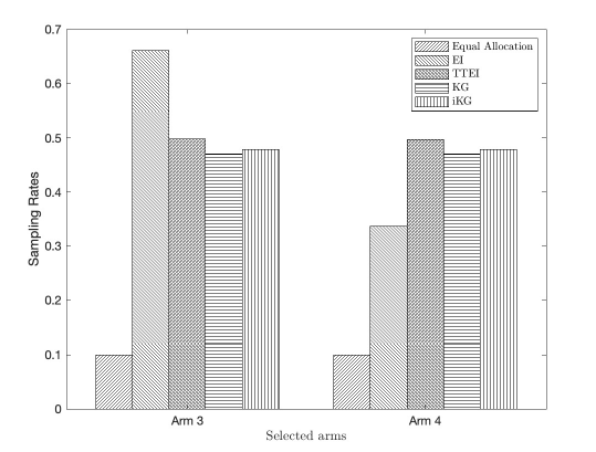
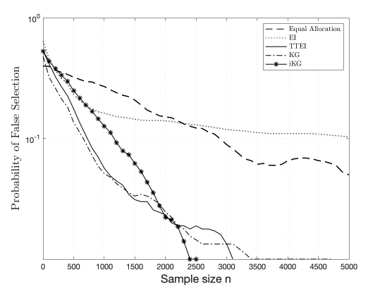
In this section, we provide additional numerical results for the experiments conducted in Section 5 of the main text. Figures 1(a)-7(a) show how the probabilities of false selection of the compared algorithms change with the sample sizes for the best arm identification problem, and Figures 1(b)-7(b) show the sampling rates of the algorithms on some selected arms. It can be observed in Figures 1(a)-7(a) that the proposed iKG algorithm performs the best, followed by TTEI, KG, EI and the equal allocation. On the log scale, the probability of false selection (PFS) values of the iKG algorithm demonstrate linear patterns, indicating the potentially exponential convergence rates. For both EI and KG, the rates of the posterior convergence are not optimal, which might influence their empirical performances. The equal allocation performs the worst in general. In Figures 1(b)-7(b), we can see that TTEI always allocates half samples to the best arm when β=0.5\beta=0.5, EI allocates too many samples to the best arm while KG allocates too few samples to the best arm.

Figures 8(a)-14(a) show how the probabilities of false selection of the compared algorithms change with the sample sizes for the ϵ\epsilon-good arm identification, and Figures 8(b)-14(b) show the sampling rates of the algorithms on some selected arms. It can be observed in Figures 8(a)-14(a) the proposed iKG-ϵ{\epsilon} algorithm performs the best and demonstrates a linear pattern on the log scale. (ST)2 and APT are inferior, and the equal allocation performs the worst. In Figures 8(b)-14(b), we can see that APT allocates too few samples to the best arm and too many samples to the arms near the threshold. ST2 allocates too few samples to the best arm, which influences the accuracy of the threshold.

Figures 15(a)-21(a) show how the probabilities of false selection of the compared algorithms change with the sample sizes for the feasible arm identification, and Figures 15(b)-21(b) show the sampling rates of the algorithms on some selected arms. The results in Figures 15(a)-21(a) are similar to those in Figures 1(a)-14(a). The proposed iKG-F algorithm has the best performance, followed by the compared MD-UCBE, equal allocation and MD-SAR. In Figures 15(b)-21(b), we can see that MD-UCBE and MD-SAR allocate too many samples to the arms near the constraint limits.

Refer to caption
Refer to caption
Figure 1: PFS and sampling rates of selected arms for the best arm identification (Example 1)
Refer to caption
Refer to caption
Figure 2: PFS and sampling rates of selected arms for the best arm identification (Example 2)
Refer to caption
Refer to caption
Figure 3: PFS and sampling rates of selected arms for the best arm identification (Example 3)
Refer to caption
Refer to caption
Figure 4: PFS and sampling rates of selected arms for the best arm identification (Dose-Finding Problem)
Refer to caption
Refer to caption
Figure 5: PFS and sampling rates of selected arms for the best arm identification (Drug Selection Problem)
Refer to caption
Refer to caption
Figure 6: PFS and sampling rates of selected arms for the best arm identification (Caption 853)
Refer to caption
Refer to caption
Figure 7: PFS and sampling rates of selected arms for the best arm identification (Caption 854)
Refer to caption
Refer to caption
Figure 8: PFS and sampling rates of selected arms for the ϵ\epsilon-good arm identification (Example 1)
Refer to caption
Refer to caption
Figure 9: PFS and sampling rates of selected arms for the ϵ\epsilon-good arm identification (Example 2)
Refer to caption
Refer to caption
Figure 10: PFS and sampling rates of selected arms for the ϵ\epsilon-good arm identification (Example 3)
Refer to caption
Refer to caption
Figure 11: PFS and sampling rates of selected arms for the ϵ\epsilon-good arm identification (Dose-Finding Problem)
Refer to caption
Refer to caption
Figure 12: PFS and sampling rates of selected arms for the ϵ\epsilon-good arm identification (Drug Selection Problem)
Refer to caption
Refer to caption
Figure 13: PFS and sampling rates of selected arms for the ϵ\epsilon-good arm identification (Caption 853)
Refer to caption
Refer to caption
Figure 14: PFS and sampling rates of selected arms for the ϵ\epsilon-good arm identification (Caption 854)
Refer to caption
Refer to caption
Figure 15: PFS and sampling rates of selected arms for the feasible arm identification (Example 1)
Refer to caption
Refer to caption
Figure 16: PFS and sampling rates of selected arms for the feasible arm identification (Example 2)
Refer to caption
Refer to caption
Figure 17: PFS and sampling rates of selected arms for the feasible arm identification (Example 3)
Refer to caption
Refer to caption
Figure 18: PFS and sampling rates of selected arms for the feasible arm identification (Dose-Finding Problem)
Refer to caption
Refer to caption
Figure 19: PFS and sampling rates of selected arms for the feasible arm identification (Drug Selection Problem)
Refer to caption
Refer to caption
Figure 20: PFS and sampling rates of selected arms for the feasible arm identification (Caption 853)
Refer to caption
Refer to caption
Figure 21: PFS and sampling rates of selected arms for the feasible arm identification (Caption 854)