Improving Robustness to Model Inversion Attacks via Mutual Information Regularization

In MI attacks, an adversary, given the access to a target model $f$ trained to predict specific labels $Y$, uses it to infer the information about the training data distribution $X$. We denote the output of the target model as $\hat{Y}$, i.e., $\hat{Y}=f(X)$. In addition, the adversary may also have access to some auxiliary knowledge $T$ that facilitates the inference. Consider the MI attacks against a face recognition model that labels an image containing a face with an identity corresponding to the individual depicted in the image. The attack goal is to recover a representative image for some target identity $y$ based on the access to the target model. Possible auxiliary knowledge could be corrupted or blurred face images (Yang, Chang, and Liang 2019; Zhang et al. 2019).

For the face recognition example, both the recovery of a training image for the target identity in and that of a test image (i.e., the image that does not appear in the training set but drawn from the same distribution) would incur privacy loss to the individual. Hence, it is important to design defenses to ensure the privacy of the entire training distribution, rather than just the members in training set. The goal of our defense is to design an algorithm to train the target model $f$ on the data distribution $(X,Y)$ such that the access to the resulting model does not allow an adversary to infer the information about $P(X|\hat{Y}=y)$.

A naive defense is to produce a classifier where $\hat{Y}$ is independent of $X$. In this case, the adversary cannot learn anything about the input data distribution for a given label. However, this classifier would clearly be useless in practice. Hence, there is a tradeoff between privacy and model utility and we want a defense that can achieve the best tradeoff between the two.

Intuitively, we will need to limit the dependency between $X$ and $\hat{Y}$ to prevent the adversary from inferring the training data distribution associated with a specific label. Our idea is to quantify the dependence between $X$ and $\hat{Y}$ using their mutual information $\mathcal{I}(X;\hat{Y})$ and incorporate it into the training objective as a regularizer. Specifically, our defense, which we call MID, trains the target model via the following loss function:

$$\min_{f\in\mathcal{H}}E_{(x,y)\sim p_{X,Y}(x,y)}[\mathcal{L}(y,f(x))]+\lambda\mathcal{I}(X,\hat{Y})$$

(1)

where $\mathcal{I}(X,\hat{Y})=\int_{\mathcal{X}}\int_{\mathcal{Y}}p_{X,Y}(x,y)\log(\frac{p_{X,Y}(x,y)}{p_{X}(x)p_{Y}(y)})dydx$, $\mathcal{L}(y,f(x))$ is the loss function for the main prediction task, and $\lambda$ is the weight coefficient that controls the tradeoff between privacy and utility on the main prediction task.

To deconstruct the proposed regularizer, we re-write the mutual information as follows:

$$\mathcal{I}(X,\hat{Y})=\mathcal{H}(\hat{Y})-\mathcal{H}(\hat{Y}|X)$$

(2)

When $f$ is a deterministic model, $\mathcal{H}(\hat{Y}|X)=0$ and introducing the mutual information regularizer effectively reduces the entropy of the model output, i.e., $\mathcal{H}(\hat{Y})$. When $f$ is stochastic, the regularizer will additionally promote the uncertainty of the model output for a fixed input, i.e., $\mathcal{H}(\hat{Y}|X)$. In practice, reducing $\mathcal{H}(\hat{Y})$ encourages the model output to be more concentrated and different inputs to be mapped into the same or very similar outputs; increasing $\mathcal{H}(\hat{Y}|X)$ makes the output to have a larger variance for a given $x$. Both terms will make $X$ less likely to be determined from the $\hat{Y}$. Figure 1 illustrates this “two-pronged” privacy protection implied by our mutual information regularizer for a stochastic neural network consisting of a mean and a variance network trained on FaceScrub dataset. Figure 1 (a) plots the confidence value on the label class versus the sum of confidence on other classes for all test data with a particular label. It demonstrates that the regularizer will lead to more concentrated model outputs. Figure 1 (b) shows the simulated distribution of confidence values for a particular image through models trained with MID. We can see an increased trend of prediction variance for this input with increased $\lambda$, i.e. the strength of the MID regularizer.

MID provides an appealing defense principle, as it defines what we mean by an effective defense, in terms of the fundamental tradeoff between reducing the input-output dependency and retaining good predictive power. However, computing mutual information is, in general, computational expensive. It requires modeling the joint distribution of model input and output and taking an integral over both domains, which is impracticable for most of the real-world prediction tasks. Here, we present efficient methods to implement the mutual information regularizer for different ML models that have been successfully attacked by previous work, including linear regression, decision trees, and neural networks. The unified idea underlying these methods is to find a tractable approximation to the mutual information regularizer.

We present a methodology for formalizing the MI attacks. Unlike previous works that capture the privacy loss of members in the training set (Wu et al. 2016; Yeom et al. 2018), this is the first attempt of modeling the privacy loss of members in the population.

We have been mainly focused on the type of attacks that aim to recover all dimensions of the feature vector corresponding to a given label. Prior work on the MI attacks has also considered other types of attacks that only aim to reconstruct partial dimensions of the feature vector and have access to the remaining dimensions as auxiliary knowledge. For instance, Fredrikson et al. (2014) studied the MI attacks against a linear regression model that predict the medicine dosage based on the input of genotypes and some nonsensitive data like demographic information. To subsume this attack setting under our general formalization, we let the input random variable consists of the sensitive and nonsensitive part, i.e., $X=(X_{s},X_{ns})$, and the attacker has access to $X_{ns}$.

The attacker could also be interested in some specific property of the feature vector instead of the entire dimensions. In the face recognition example, the attacker could be interested in learning about the properties of a face image, such as hair color and race, instead of reconstructing the entire face image (Zhang et al. 2019). To capture this common attack scenario, we introduce $\tau$ to denote the property function that maps the sensitive feature to the property of the interest to the attacker.

We abstract the MI attacks into the following semantic MI game played between the server and the adversary. The game is described by a tuple $(\mathcal{A},\mathcal{M},p,\tau)$, where $\mathcal{A}$ denotes the adversary which is a probabilistic machine with access to the learning algorithm $\mathcal{M}$ and $p$ is the target data distribution. $\mathcal{M}:\mathcal{X}^{n}\rightarrow\mathcal{H}$ is a learning algorithm that takes a dataset as input and outputs a single, fixed classifier $f$. $\mathcal{H}$ represents the hypothesis class.

The gain of the game is evaluated as

	$\displaystyle\texttt{gain}^{\textbf{SEM}}(\mathcal{A},\mathcal{M},p,\tau)$	$\displaystyle=Pr[\mathbf{Exp^{SEM}}(\mathcal{A},\mathcal{M},p,\tau)=1]$
		$\displaystyle=Pr[\mathcal{A}_{x_{ns},y}=\tau(x_{s})]$		(6)

where the probability is taken over the randomness of $S\sim p^{n}$, the randomness of $\mathcal{M}$, the randomness of $\mathcal{A}$ and the randomness of $(x_{s},x_{ns},y)\sim p$. This game directly formalizes the procedure of MI attack. Trivially, for this game, the best strategy for the adversary is always output the most probable $\tau(x_{s})$ when $x_{s}\sim p_{X_{s}|x_{ns},y}$. Hence, the best possible gain for this game is

$$E_{(x,y)\sim p}[\max_{v}Pr_{x_{s}\sim p_{X_{s}|x_{ns},y}}[\tau(x_{s})=v]]$$

(7)

To properly measure the adversary’s advantage gained from the classifier $f$, we define an alternative underlying distribution $p_{X_{s}}\times p_{X_{ns},Y}$ such that $X_{s}$ and $(X_{ns},Y)$ have no correlation with each other. That is, sampling $x_{s}\sim p_{X_{s}}$ independently from $X_{ns}$ and $Y$. We define the advantage of $\mathcal{A}$ to be

$$\begin{split}\texttt{Adv}^{\textbf{SEM}}&(\mathcal{A},\mathcal{M},p,\tau)=\texttt{gain}^{\textbf{SEM}}(\mathcal{A},\mathcal{M},p,\tau)\\ &-\texttt{gain}^{\textbf{SEM}}(\mathcal{A},\mathcal{M},p_{X_{s}}\times p_{X_{ns},Y},\tau)\end{split}$$

(8)

i.e. $\texttt{gain}^{\textbf{SEM}}(\mathcal{A},\mathcal{M},p_{X_{s}}\times p_{X_{ns},Y},\tau)$ is the trivial baseline gain of the adversary when there are indeed no correlation between $X_{s}$ and $(X_{ns},Y)$, and $\texttt{Adv}^{\textbf{SEM}}$ measures the extra gain the adversary can get. Note that there are multiple other ways to define the adversary’s advantage which capture different insights. We defer this discussion to the Appendix.

One dominate privacy notion is DP, which carefully randomizes an algorithm so that its output does not to depend too much on any single individual in the dataset (Dwork, Roth et al. 2014).

We introduce an indistinguishability game to derive the robustness guarantee offered by DP. The game is described by a tuple $(\mathcal{A},\mathcal{M},p)$.

Let $\texttt{gain}^{\textbf{IND}}\!(\mathcal{A},\mathcal{M},p)\!=Pr[\mathbf{Exp^{IND}}(\mathcal{A},\mathcal{M},p)=1]$. The following theorem shows that the gain of the semantic MI game can be upper bounded in terms of the best possible gain of this indistinguishability game.

Hence, to mitigate the threats of MI attack, we want $\max_{\mathcal{A}}\texttt{gain}^{\textbf{IND}}$ to be not much greater than $1/2$.

We will provide a tight bound of $\texttt{gain}^{\textbf{IND}}$ for any attack strategy $\mathcal{A}$ when the learning algorithm is differentially private. In the analysis, we assume that with high probability a training set drawn from $p^{n}$ has no intersection with another set drawn from $(p_{X_{s}}\times p_{X_{ns},Y})^{n}$, i.e.,

$$Pr_{S\sim p^{n},S^{\prime}\sim(p_{X_{s}}\times p_{X_{ns},Y})^{n}}[S\sim_{n}S^{\prime}]=1-\gamma$$

(11)

where $S\sim_{n}S^{\prime}$ indicates that the two datasets $S,S^{\prime}\in\mathcal{X}^{n}$ differ by $n$ entries, and $\gamma$ is a small value. This assumption is plausible for many practical scenarios where the feature vector has continuous domain or is high-dimensional.

As we can see, to make the upper bound $\frac{e^{n\epsilon}}{e^{n\epsilon}+1}+\frac{e^{n\epsilon}-1}{(e^{n\epsilon}+1)(e^{\epsilon}-1)}\delta=\frac{1}{2}+\frac{e^{n\epsilon}-1}{2(e^{n\epsilon}+1)}+\frac{e^{n\epsilon}-1}{(e^{n\epsilon}+1)(e^{\epsilon}-1)}\delta\in\frac{1}{2}+o(1)$, the privacy budget $\epsilon$ needs to be set as $o(\frac{1}{n})$. However, this privacy budget is too small to allow any useful computation (see, e.g., Section 2.3.3 of Dwork, Roth et al. (2014), for a comprehensive review). Since the bound in Theorem 2 is tight, with high probability DP cannot mitigate the MI attacks with any reasonable model utility.

Table 1 summarizes our experimental setting, including the attacks, models, datasets, metrics used in our evaluation as well as the other defenses that we compare with. We leave the description of datasets, attack hyper-parameters, model architectures as well as the details of the evaluation process and metrics to the Appendix.

Figure 2 compares the performance of our defense against the existing baselines on various blackbox attacks, including Naive MAP (Figure 2 (a-b)), Knowledge Alignment (Figure 2 (c)), and Update-Leaks (Figure 2 (d)). For Naive MAP, we demonstrate the results on both linear regression and decision trees as these two models were successfully attacked by Naive MAP in prior work (Fredrikson et al. 2014; Fredrikson, Jha, and Ristenpart 2015). Knowledge Alignment and Update-Leaks are designed for attacking neural networks, so we only exhibit the results on neural networks for these two attacks. Figure 2 shows that MID can consistently achieve a better utility-privacy tradeoff than DP for protecting against all the attacks. For decision trees, there exists a model-specific defense strategy, named Priority, which adjusts the depth of the sensitive feature. Figure 2 (b) shows that MID is more robust than Priority in most cases except when model has a very high performance (i.e., F1 score $>$ 0.57). Nevertheless, Priority has its own drawbacks: firstly, it is only applicable to decision trees; and second, it only protects a subset of attributes, or the sensitive attributes, which could be subject to additional privacy concern because one may leverage the correlation between nonsensitive attributes and sensitive attributes to recover the sensitive one. On the other hand, the principles of MID and DP are applicable to different types of models and protect all the attributes at once. A phenomenon consistently present in all attacks is that the more predictive power the model has, the more vulnerable it is to the attacks, regardless of the types of defenses attached to the model. This finding signifies the difficulty to defend against the MI attacks; yet, our defense can significantly improve the model robustness for any fixed model performance. We also evaluate the attack performance in terms of other metrics shown in Table 1. As they give the similar results to the metrics exhibited in Figure 2, we will omit these results to the Appendix.

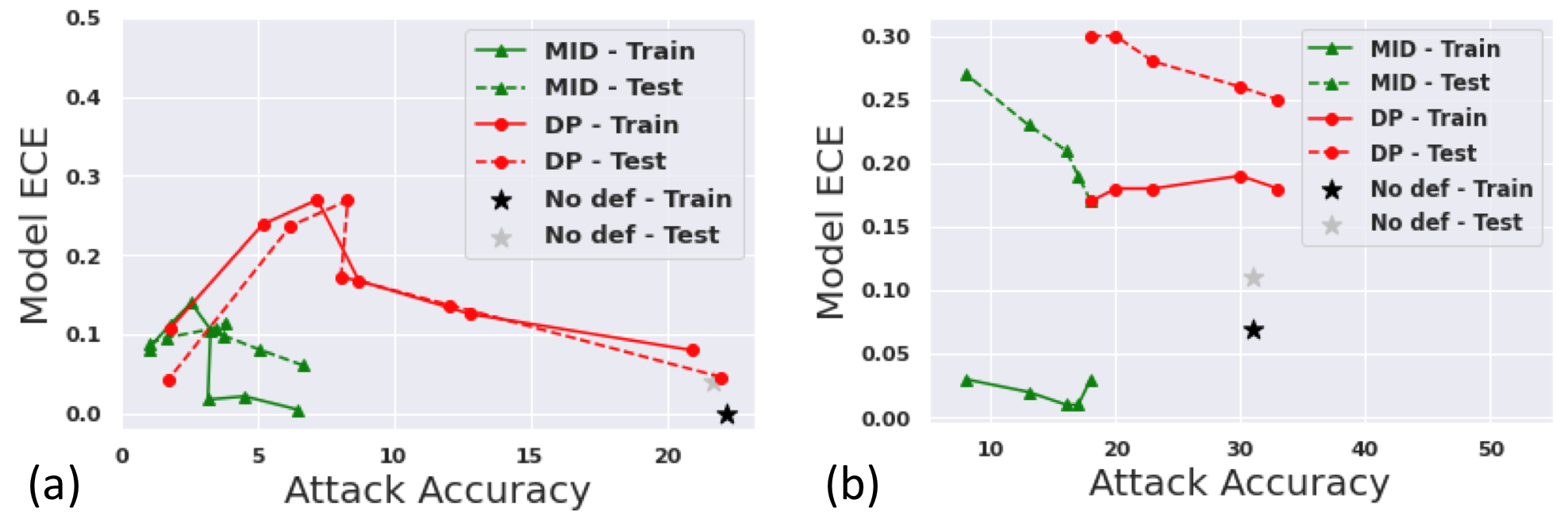
Figure 3 illustrates the miscalibration between confidence and accuracy as the result of different defenses. The degree of miscalibration is measured by ECE. We find that MID mostly achieves significantly lower ECE error than DP for a given robustness level.

Figure 4 illustrates the defense results for whitebox attacks. Specifically, we consider GMI, the state-of-the-art attack against neural networks, and MAP with counts, the only known attack against decision trees; the corresponding privacy-utility tradeoff curves are shown in Figure 4 (b) and (c), respectively. We find that MID can outperform DP by a large margin to defend against whitebox MI attacks. Similar to the observation in blackbox experiment, model-specific defense strategies could achieve better robustness than MID occasionally; but overall, MID could be more preferable due to its broad applicability, thorough protection for all attributes, and reliable performance. Figure 4 (a) compares the reconstructed images of MID and DP. We tune the hyperparameters of both defenses so that the resulting target models have comparable performance. The test accuracies for the models trained with MID and DP are 80.8 and 81.4, respectively. We can see that MID can block the attack much better than DP. For instance, the reconstructions for DP can still retain many facial features of the target individual while the reconstructions for MID are almost completely different from the target individual.

One common observation from all defense results is that the attack performance is very close on training and test set. This implies that MI attacks pose similar privacy threats regardless of whether an individual’s data is selected for training or not. Although some prior works (Yeom et al. 2018; Dwork et al. 2015) report that the attack performance on the training set is much higher than the test set, we conjecture that it is because the model overfits the training data in their evaluations. In our experiments, since both MID and DP can help mitigate overfitting, the privacy threats of MI attacks is presented to the population instead of the training set only.

The utility metrics depend on the underlying prediction task and datasets. For regression tasks, we employ mean squared error (MSE); for classification tasks, we generally use test accuracy as the metric unless the dataset is highly imbalanced in which case we use the F1 score. For blackbox attacks on neural networks, there is a trivial defense to just release the prediction rather than the entire confidence vector and this defense achieves good utility in terms of test accuracy. However, this defense omits useful confidence information.

To evaluate the impact of defense algorithm on the precision of confidence information, we measure the degree of model calibration in terms of Expected Calibration Error (ECE) for each different model (Guo et al. 2017). We say that the defense A dominates the defense B if A can achieve better robustness than B when their model performance is fixed to any value (in some reasonable range). Model calibration is the degree to which a model’s predicted probability estimates the true correctness likelihood. ECE measures the difference in expected accuracy and expected confidence. In practice, we group predictions into $M$ bins, and let $B_{m}$ be the set of indices of samples whose prediction confidence falls into the interval $I_{m}=(\frac{m-1}{M},\frac{m}{M}]$ for $m\in\{1\dots,M\}$. ECE is then computed as

$$\sum_{m=1}^{M}\frac{|B_{m}|}{n}|acc(B_{m})-conf(B_{m})|$$

where $acc(B_{m})=\frac{\sum_{i\in B_{m}}I[\arg\max_{y}\hat{y}_{i}=y_{i}]}{|B_{m}|}$ and $conf(B_{m})=\frac{1}{|B_{m}|}\sum_{i\in B_{m}}\hat{p}_{i}$, where $\hat{p}_{i}$ is the confidence for sample $i$ on label $y_{i}$.

As for the attack performance, we follow the papers where the attacks were originally proposed and mostly use their metrics. There are three metrics to measure the attack performance when the target sensitive attribute is discrete: (1) accuracy, which is the percentage of samples for which the attack algorithm correctly predicted genotype, (2) AUROC, which is the multi-class area under receiver operating characteristic (ROC) curve, and (3) F1-score, which is the harmonic average of attack precision and recall. This is because in both IWPC and FiveThirtyEight the distribution of the target attribute is highly unbalanced. Although attack accuracy is generally easier to interpret, it can be misleading in this case. AUROC and F1-score are intended to help evaluating when the sensitive attributes are highly imbalanced.

For MI attacks on image recognition model, L2 Distance is measured between the original and reconstructed images. We also build an evaluation classifier to evaluate the attack accuracy on neural network models. If the evaluation classifier can correctly classify the reconstructed image, then the image is considered to be close to a representative image for a certain label class. The evaluation classifier is different from the target classifier and has very high performance, which serves as a label predicting oracle. For knowledge alignment experiment (FaceScrub), our evaluation network is adapted from VGG-16 (Simonyan and Zisserman 2014). For GMI experiment (CelebA), we use the model in (Cheng et al. 2017) which is pretrained on the MS-Celeb-1M (Guo et al. 2016) and then fine-tuned on the training set of the target network.

We present defense results for blackbox and whitebox MI attacks measured with additional metrics. Figure 5 shows that our proposed defense outperforms DP on these additional metrics. Comparing Figure 5 (b) with (c), we found that training data are subject to a higher privacy loss than test data for the model attacked by GMI, while the privacy loss of training and test data is about the same for the model attacked by Knowledge distillation. One potential reason is that the model in (c) has more parameters and thus is subject to more overfitting. If the model overfits to training data, the model tends to learn the input-output correlation better for training data than test data and as a result, training data is more susceptible to MI attacks. Another potential reason is that the attack algorithm in (c) is more powerful as it is a whitebox attack while the attack in (b) only has blackbox access to the model. Hence, the attack in (c) can better reflect the subtle difference between training and test data in terms of their vulnerability. We leave the validation of these hypotheses to future work.

There are several possible ways to define the trivial baseline of the attack gain. A common practice in cryptography is to define a simulator $\mathcal{S}$ which has access to everything else but the target model $f$:

$$\mathcal{S}(\mathcal{A},p,\tau)=Pr_{\mathcal{A},(x_{s},x_{ns},y)\sim p}[\mathcal{A}_{x_{ns},y}=\tau(x_{s})]$$

(12)

and the advantage of $\mathcal{A}$ can be defined as

$$\texttt{Adv}^{\textbf{SEM}}_{\mathcal{S}}(\mathcal{A},f,p,\tau)=\texttt{gain}^{\textbf{SEM}}(\mathcal{A},\mathcal{M},p,\tau)-\mathcal{S}(\mathcal{A},p,\tau)$$

(13)

Another potential baseline definition is to define an alternative underlying distribution $p_{X_{s}}\times p_{X_{ns},Y}$ such that $X_{s}$ and $(X_{ns},Y)$ have no correlation with each other. That is, sampling $x_{s}\sim p_{X_{s}}$ independently from $X_{ns}$ and $Y$. We then define another classifier $f^{*}$ that is trained from a training set $S$ draws from $p_{X_{s}}\times p_{X_{ns},Y}$, and define the advantage of $\mathcal{A}$ to be

$$\begin{split}\texttt{Adv}^{\textbf{SEM}}(\mathcal{A},f,p,&\tau)=\texttt{gain}^{\textbf{SEM}}(\mathcal{A},\mathcal{M},p,\tau)\\ &-\texttt{gain}^{\textbf{SEM}}(\mathcal{A},\mathcal{M},p_{X_{s}}\times p_{X_{ns},Y},\tau)\end{split}$$

(14)

This definition captures the intuition that if $X_{s}$ has little correlation with $X_{ns}$ and $Y$, the advantage of the attacker should be small no matter which strategy he/she uses and which classifier $f$ it has access to. We can also define an alternative experiment:

In this experiment, the classifier $f$ still provides correlation information between $X_{ns}$ and $Y$ but no longer contain information for the correlation between $X_{s}$ and $(X_{ns},Y)$, thus it’s information-theoretically hard to compute $\tau(x_{s})$. Using this experiment, we can have another definition of the advantage of $\mathcal{A}$:

$$\begin{split}&\texttt{Adv}^{\textbf{SEM}}(\mathcal{A},f,p,\tau)\\ &=\texttt{gain}^{\textbf{SEM}}(\mathcal{A},\mathcal{M},p,\tau)-\texttt{gain}^{\textbf{SEM}}_{\textbf{ideal}}(\mathcal{A},\mathcal{M},p,\tau)\end{split}$$

(15)

We will provide a tight bound of $\texttt{gain}^{\textbf{IND}}$ for any attack strategy $\mathcal{A}$ when the learning algorithm is differentially private. In the analysis, we assume that with high probability a training set drawn from $p^{n}$ has no intersection with another set drawn from $(p_{X_{s}}\times p_{X_{ns},Y})^{n}$, i.e.,

$$Pr_{S\sim p^{n},S^{\prime}\sim(p_{X_{s}}\times p_{X_{ns},Y})^{n}}[S\sim_{n}S^{\prime}]=1-\gamma$$

(32)

where $S\sim_{n}S^{\prime}$ indicates that the two datasets $S,S^{\prime}\in\mathcal{X}^{n}$ differ by $n$ entries, and $\gamma$ is a small value. This assumption is plausible for many practical scenarios where the feature vector has continuous domain or is high-dimensional.

References

- Abadi et al. (2016) Abadi, M.; Chu, A.; Goodfellow, I.; McMahan, H. B.; Mironov, I.; Talwar, K.; and Zhang, L. 2016. Deep learning with differential privacy. In Proceedings of the 2016 ACM SIGSAC Conference on Computer and Communications Security, 308–318.
- Alemi et al. (2016) Alemi, A. A.; Fischer, I.; Dillon, J. V.; and Murphy, K. 2016. Deep variational information bottleneck. arXiv preprint arXiv:1612.00410 .
- Cheng et al. (2017) Cheng, Y.; Zhao, J.; Wang, Z.; Xu, Y.; Jayashree, K.; Shen, S.; and Feng, J. 2017. Know you at one glance: A compact vector representation for low-shot learning. In Proceedings of the IEEE International Conference on Computer Vision Workshops, 1924–1932.
- Cover (1999) Cover, T. M. 1999. Elements of information theory. John Wiley & Sons.
- Dwork et al. (2015) Dwork, C.; Feldman, V.; Hardt, M.; Pitassi, T.; Reingold, O.; and Roth, A. 2015. Generalization in adaptive data analysis and holdout reuse. In Advances in Neural Information Processing Systems, 2350–2358.
- Dwork, Roth et al. (2014) Dwork, C.; Roth, A.; et al. 2014. The algorithmic foundations of differential privacy. Foundations and Trends® in Theoretical Computer Science 9(3–4): 211–407.
- Fredrikson, Jha, and Ristenpart (2015) Fredrikson, M.; Jha, S.; and Ristenpart, T. 2015. Model inversion attacks that exploit confidence information and basic countermeasures. In Proceedings of the 22nd ACM SIGSAC Conference on Computer and Communications Security, 1322–1333.
- Fredrikson et al. (2014) Fredrikson, M.; Lantz, E.; Jha, S.; Lin, S.; Page, D.; and Ristenpart, T. 2014. Privacy in pharmacogenetics: An end-to-end case study of personalized warfarin dosing. In 23rd USENIX Security Symposium (USENIX Security 14), 17–32.
- Friedman and Schuster (2010) Friedman, A.; and Schuster, A. 2010. Data mining with differential privacy. In Proceedings of the 16th ACM SIGKDD international conference on Knowledge discovery and data mining, 493–502.
- Guo et al. (2017) Guo, C.; Pleiss, G.; Sun, Y.; and Weinberger, K. Q. 2017. On calibration of modern neural networks. arXiv preprint arXiv:1706.04599 .
- Guo et al. (2016) Guo, Y.; Zhang, L.; Hu, Y.; He, X.; and Gao, J. 2016. Ms-celeb-1m: A dataset and benchmark for large-scale face recognition. In European conference on computer vision, 87–102. Springer.
- Huber et al. (2008) Huber, M. F.; Bailey, T.; Durrant-Whyte, H.; and Hanebeck, U. D. 2008. On entropy approximation for Gaussian mixture random vectors. In 2008 IEEE International Conference on Multisensor Fusion and Integration for Intelligent Systems, 181–188. IEEE.
- Kolchinsky, Tracey, and Wolpert (2019) Kolchinsky, A.; Tracey, B. D.; and Wolpert, D. H. 2019. Nonlinear information bottleneck. Entropy 21(12): 1181.
- Quinlan (1986) Quinlan, J. R. 1986. Induction of decision trees. Machine learning 1(1): 81–106.
- Salem et al. (2019) Salem, A.; Bhattacharya, A.; Backes, M.; Fritz, M.; and Zhang, Y. 2019. Updates-leak: Data set inference and reconstruction attacks in online learning. arXiv preprint arXiv:1904.01067 .
- Shwartz-Ziv and Tishby (2017) Shwartz-Ziv, R.; and Tishby, N. 2017. Opening the black box of deep neural networks via information. arXiv preprint arXiv:1703.00810 .
- Simonyan and Zisserman (2014) Simonyan, K.; and Zisserman, A. 2014. Very deep convolutional networks for large-scale image recognition. arXiv preprint arXiv:1409.1556 .
- Wang (2018) Wang, Y.-X. 2018. Revisiting differentially private linear regression: optimal and adaptive prediction & estimation in unbounded domain. arXiv preprint arXiv:1803.02596 .
- Wu et al. (2016) Wu, X.; Fredrikson, M.; Jha, S.; and Naughton, J. F. 2016. A methodology for formalizing model-inversion attacks. In 2016 IEEE 29th Computer Security Foundations Symposium (CSF), 355–370. IEEE.
- Yang, Chang, and Liang (2019) Yang, Z.; Chang, E.-C.; and Liang, Z. 2019. Adversarial neural network inversion via auxiliary knowledge alignment. arXiv preprint arXiv:1902.08552 .
- Yang et al. (2020) Yang, Z.; Shao, B.; Xuan, B.; Chang, E.-C.; and Zhang, F. 2020. Defending Model Inversion and Membership Inference Attacks via Prediction Purification. arXiv preprint arXiv:2005.03915 .
- Yeom et al. (2018) Yeom, S.; Giacomelli, I.; Fredrikson, M.; and Jha, S. 2018. Privacy risk in machine learning: Analyzing the connection to overfitting. In 2018 IEEE 31st Computer Security Foundations Symposium (CSF), 268–282. IEEE.
- Zhang et al. (2019) Zhang, Y.; Jia, R.; Pei, H.; Wang, W.; Li, B.; and Song, D. 2019. The Secret Revealer: Generative Model-Inversion Attacks Against Deep Neural Networks. arXiv preprint arXiv:1911.07135 .
Appendix A: Additional Experiment Details
We give more details of datasets, evaluation metrics, as well as different attack experiments here. We also submit our code as part of the supplementary materials.
Datasets
IWPC
The IWPC collected data on patients who were prescribed warfarin in 9 counties. 17 attributes of the patients are collected including a genotype VKORC1, which is considered as the target sensitive attributes in our paper. The outcome variable is the stable therapeutic dose of Warfarin. This dataset is considered as a benchmark dataset for linear regression inversion attack (Fredrikson et al. 2014). Note that in (Fredrikson et al. 2014), another genotype CYP2C9 is also considered as sensitive target, but since CYP2C9 has low correlation with dosage and demographic information, we show the attacking results on VKORC1 only.
FiveThirtyEight
FiveThirtyEight is a survey of 553 individuals from SurveyMonkey which support the analysis of the connection between peoples’ steak preparation preferences and their propensity for risk-taking behaviors. The response for the question about infidelity is considered sensitive, following the settings in (Fredrikson, Jha, and Ristenpart 2015).
FaceScrub
A dataset of 48,579 images for 530 individuals. We extract the face of each image according to the official bounding box information. Each image is resized to , following the settings in (Yang, Chang, and Liang 2019).
CelebA
the CelebFaces Attributes Dataset (CelebA) containing 202,599 face images of 10,177 identities with coarse alignment. We crop the images at the center and resize them to so as to remove most background, following the settings in (Zhang et al. 2019).
CIFAR10
A dataset consists of 60,000 images in 10 classes (airplane, automobile, bird, cat, deer, dog, frog, horse, ship and truck). Each image is resized to .
Utility Metrics