Improving NASA/IPAC Extragalactic Database Redshift Calculations

Velocities are a complex topic in cosmology because they are coordinate dependent and we generally use coordinates that violate some of our naïve expectations of velocity behavior. This is in contrast to redshifts, that are observable, dimensionless ratios and thus unambiguous.

The low-redshift approximation $z=v/c$ is appropriate for both peculiar velocities and (small) recession velocities. However, the two types of velocities are quite different. Peculiar velocities, $v_{\rm p}$, are measured with respect to a local Minkowski (special relativistic) frame, and thus the redshift induced by a velocity obeys the special relativistic Doppler shift formula,

On the other hand, the recession velocity that appears in the Hubble–Lemaître law, $v_{\rm r}$, cannot be described in any inertial frame. It can be derived from the Friedmann–Lemaître–Robertson–Walker metric as the purely expansion component of the time derivative of proper distance, $D$ (Davis & Lineweaver, 2004). The other component, from changes in comoving coordinate caused by gravitation, are the peculiar velocities above. Indeed for $v_{\rm r}=H_{0}D$ to be true at any $D$, $v_{\rm r}$ must be allowed to exceed the speed of light. (An analogous situation occurs with superluminal infall velocities of “space” inside a black hole, which is why light cannot escape.) This is a standard result, which is a requirement for homogeneity and isotropy, and does not violate relativity. Thus recession velocities do not obey the special relativistic Doppler shift formula, but are instead calculated by integrating over the expansion rate of the universe during the photon’s propagation (Harrison, 1993),

where the dimensionless Hubble parameter $E(z)=H(z)/H_{0}=\sqrt{\sum\Omega_{i}(1+z)^{3(1+w_{i})}}$ (Peebles, 1993; Ryden, 2003) with $H(z)$ being the Hubble parameter at the time of emission from a galaxy at redshift $z$, $\Omega_{i}$ being the normalized density of component $i$ of the universe, and $w_{i}$ being that component’s equation of state. It is interesting to note that the recession velocity as a function of redshift is actually independent of $H_{0}$.

The total velocity, $v_{\rm t}$, of an object moving away from us can be accurately calculated as $v_{\rm t}=v_{\rm r}+v_{\rm p}$ (Davis & Lineweaver, 2004). The common additive approximation for redshifts comes from dividing this equation by $c$ and applying the low-$z$ approximation $z=v/c$. However, given the current precision of other measurements, this will be a poor approximation for any redshift higher than $z\sim 0.01$.

To correct $z_{\mathrm{obs}}$ to the CMB frame requires finding $z_{\mathrm{p,Sun}}^{\mathrm{{}}}$. The motion of the solar system adds a peculiar redshift to every object. That peculiar redshift is highest for objects that are in or directly opposite the direction of motion, resulting in a maximum $z_{\mathrm{p,Sun}}^{\mathrm{{}}}$ of order 10^-3. The effective radial peculiar velocity of any object is the projection of the Sun’s velocity vector on the position vector of the object,

where $v_{\mathrm{p,Sun}}^{\mathrm{{}}}$ represents the projection of the Sun’s peculiar velocity along the line of sight to the object, $\hat{\textit{{n}}}_{\text{obj}}$ is the object’s position vector, and $\alpha$ is the angle separating the dipole direction and the object.²²2The formula for the angular separation, $\alpha$, in terms of galactic longitude and latitude, $(l,b)$, is $$\cos\alpha=\sin(b)\sin(b_{0})+\cos(b)\cos(b_{0})\cos(l-l_{0}),$$ (7) where $(l_{0},b_{0})$ correspond to the dipole direction. An equivalent calculation that is more numerically stable at very small and large separations is the Vincenty formula (Vincenty, 1975), for which we use Astropy’s SkyCoord implementation. Setting $\Delta l=l-l_{0}$, it reads as $$\tan\alpha=\frac{\sqrt{\left(\cos b_{0}\sin\Delta l\right)^{2}+\left(\cos b\sin b_{0}-\sin b\cos b_{0}\cos\Delta l\right)^{2}}}{\sin b\sin b_{0}+\cos b\cos b_{0}\cos\Delta l}.$$ (8)

We define both recession and peculiar velocities to be positive when they are moving away from us. Note that in the case of our own motion, a positive velocity gives a negative redshift (blueshift) because we are moving toward the object being observed.

Since the Sun’s velocity is small (order of 10² km s^-1) compared to $c$, the low-$z$ approximation $z_{\mathrm{p,Sun}}^{\mathrm{{}}}\approx-v_{\mathrm{p,Sun}}^{\mathrm{{}}}/c$ can be used. However, there is negligible computational disadvantage to using the full special relativistic calculation Eq. (4),

The minus signs before $v_{\mathrm{p,Sun}}^{\mathrm{{}}}$ have been left explicit to ensure that a zero separation ($\alpha=0$ in Eq. (6)) results in the object appearing blueshifted due the our positive velocity toward it. For the purposes of the plots and equations in this paper, we emphasize that we use the approximation purely for clarity and so our comparisons with NED are cleaner (since it makes negligible difference relative to the size of the other discrepancies).

The correction requires the direction and magnitude of the CMB dipole, which was measured in 2018 by the Planck Collaboration (Planck Collaboration et al., 2020) to be in the direction of $(l,b)=(264.021^{\circ}{}\pm 0.011^{\circ}{},48.253^{\circ}{}\pm 0.005^{\circ}{})$ with a velocity $v_{\mathrm{p,Sun}}^{\mathrm{{Planck}}}=369.82\pm 0.11$ km s^-1. However, NED currently uses the older measurement of the dipole by the Cosmic Background Explorer (COBE) satellite (Fixsen et al., 1996), $(l,b)=(264.14^{\circ}{}\pm 0.30^{\circ}{},48.26^{\circ}{}\pm 0.30^{\circ}{})$ with a velocity $v_{\mathrm{p,Sun}}^{\mathrm{{COBE}}}=371\pm 1$ km s^-1.³³3https://ned.ipac.caltech.edu/Documents/Guides/Calculators

We compare the different combinations of dipole and heliocentric correction form below. Performing the multiplicative correction, Eq. (2), with the modern dipole measurement is naturally the most accurate. However, we show explicitly NED uses the additive expansion, Eq. (1), and the COBE dipole. In doing so, we demonstrate the size of the resulting systematic errors currently in NED, as well as in the cases of only updating the heliocentric correction form or dipole separately.

In Figs. 2–5, we compare the CMB redshifts from NED to the CMB redshifts we calculate. We begin by confirming that NED currently uses the additive redshift calculation and the COBE dipole. In Fig. 2, we show there is negligible difference in $z_{\mathrm{CMB}}^{\mathrm{+,COBE}}-z_{\mathrm{CMB}}^{\mathrm{NED}}$ since the absolute error only reaches 5$\times 10^{-7}$. This error comes purely from comparing the NED redshifts, that are rounded to six decimal places, with our non-rounded calculations.

We then improve on the NED redshifts by using the full multiplicative heliocentric correction and the Planck dipole. Using the multiplicative redshift calculations results in a redshift difference between our calculations and NED’s on the order of 10^-3(Fig. 3), while changing the dipole results in a redshift difference on the order of 10^-6–10^-5 (Figs. 4 and 5). Correcting the current NED CMB redshift calculation is therefore the most important change, while updating the COBE dipole is a valuable but subtle change.

Figure 3 shows the full difference between the Planck dipole with multiplicative redshift calculation, and the COBE dipole with additive redshift calculation. That is the difference between Eq. (2) and Eq. (1) that we calculate analytically to be

Recall that the dipoles differ in both magnitude and direction so there are the two separate expressions for the Sun’s peculiar redshift $cz_{\mathrm{p,Sun}}^{\mathrm{{Planck}}}\approx-v_{\mathrm{p,Sun}}^{\mathrm{{max,Planck}}}\cos\alpha^{\rm Planck}$, and similar for COBE. We show in Fig. 3 these analytic calculations (Eq. (10)) by varying either $z_{\mathrm{CMB}}^{\mathrm{}}$ or $\alpha$, as dashed lines. The excellent agreement when replacing $z_{\mathrm{CMB}}^{\mathrm{NED}}$ with $z_{\mathrm{CMB}}^{\mathrm{+,COBE}}$ confirms that indeed $z_{\mathrm{CMB}}^{\mathrm{NED}}=z_{\mathrm{CMB}}^{\mathrm{+,COBE}}$.

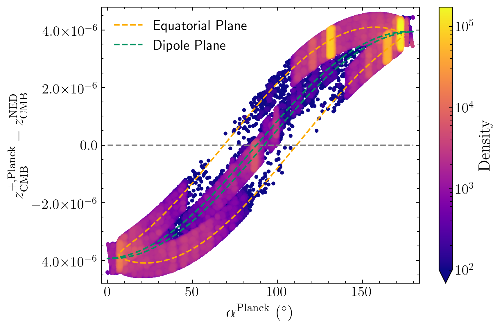
Figure 4 highlights only the difference caused by using the Planck dipole over COBE. For the purposes of this demonstration we calculate the CMB redshift using the additive approximation, but with the Planck dipole. The difference should therefore be

The more complicated shape shown in the left panel of Fig. 4 is caused by this difference in two cosines (the different dipole directions) and very clearly shows the difference between the two data samples. The dipole plane sample has a small variation about the central sinusoid since the Planck dipole is very close to the COBE dipole, but the slight offset of roughly 0.1^∘ causes a single value of $\alpha^{\mathrm{Planck}}$ to correspond to two slightly different $\alpha^{\mathrm{COBE}}$. The equatorial sample has the larger variation because closest sky position to the dipoles is 6^∘ away.

Figure 5 again compares the two dipoles, but this time using the correct multiplicative redshift calculation for both,

Comparing $z_{\mathrm{CMB}}^{\mathrm{\times,Planck}}$ to $z_{\mathrm{CMB}}^{\mathrm{NED}}$ would be only imperceptibly different from Fig. 3, so instead we opt to show the difference purely caused by the dipoles. This is essentially Fig. 4 and Eq. (11) with a multiplicative $1+z_{\mathrm{CMB}}^{\mathrm{}}$ factor. Therefore, using the full heliocentric correction with the outdated dipole measurement actually also multiplies the error. Note, however, that the sign of error when comparing dipoles is opposite to the additive versus multiplicative correction. The increased error here then cancels slightly more with the heliocentric correction form error (albeit still two orders of magnitude smaller).

References

- Calcino & Davis (2017) Calcino, J., & Davis, T. 2017, J. Cosmology Astropart. Phys, 2017, 038, doi: 10.1088/1475-7516/2017/01/038
- Chaves-Montero et al. (2018) Chaves-Montero, J., Angulo, R. E., & Hernández-Monteagudo, C. 2018, MNRAS, 477, 3892, doi: 10.1093/mnras/sty924
- Colless (1995) Colless, M. 1995, AJ, 109, 1937, doi: 10.1086/117419
- Davis et al. (2019) Davis, T. M., Hinton, S. R., Howlett, C., & Calcino, J. 2019, MNRAS, 490, 2948, doi: 10.1093/mnras/stz2652
- Davis & Lineweaver (2004) Davis, T. M., & Lineweaver, C. H. 2004, PASA, 21, 97, doi: 10.1071/AS03040
- Fixsen et al. (1996) Fixsen, D. J., Cheng, E. S., Gales, J. M., et al. 1996, ApJ, 473, 576, doi: 10.1086/178173
- Freedman et al. (2019) Freedman, W. L., Madore, B. F., Hatt, D., et al. 2019, ApJ, 882, 34, doi: 10.3847/1538-4357/ab2f73
- Glanville et al. (2021) Glanville, A., Howlett, C., & Davis, T. M. 2021, MNRAS, 503, 3510, doi: 10.1093/mnras/stab657
- Harrison (1993) Harrison, E. 1993, ApJ, 403, 28, doi: 10.1086/172179
- Peebles (1993) Peebles, P. J. E. 1993, Principles of Physical Cosmology, Princeton series in physics (Princeton University Press)
- Planck Collaboration et al. (2020) Planck Collaboration, Aghanim, N., Akrami, Y., et al. 2020, A&A, 641, A1, doi: 10.1051/0004-6361/201833880
- Riess et al. (2019) Riess, A. G., Casertano, S., Yuan, W., Macri, L. M., & Scolnic, D. 2019, ApJ, 876, 85, doi: 10.3847/1538-4357/ab1422
- Ryden (2003) Ryden, B. S. 2003, Introduction to Cosmology (Addison-Wesley)
- Slipher (1921) Slipher, V. M. 1921, PA, 29, 128
- Steinhardt et al. (2020) Steinhardt, C. L., Sneppen, A., & Sen, B. 2020, ApJ, 902, 14, doi: 10.3847/1538-4357/abb140
- The Astropy Collaboration et al. (2018) The Astropy Collaboration, Price-Whelan, A. M., Sipőcz, B. M., et al. 2018, AJ, 156, 123, doi: 10.3847/1538-3881/aabc4f
- Tonry & Davis (1979) Tonry, J., & Davis, M. 1979, AJ, 84, 1511, doi: 10.1086/112569
- Vincenty (1975) Vincenty, T. 1975, Survey Review, 23, 88, doi: 10.1179/sre.1975.23.176.88
- Wojtak et al. (2015) Wojtak, R., Davis, T. M., & Wiis, J. 2015, J. Cosmology Astropart. Phys, 2015, 025, doi: 10.1088/1475-7516/2015/07/025
- Wong et al. (2020) Wong, K. C., Suyu, S. H., Chen, G. C. F., et al. 2020, MNRAS, 498, 1420, doi: 10.1093/mnras/stz3094
- Zwicky (1933) Zwicky, F. 1933, AcHPh, 6, 110