Improved randomized neural network methods with boundary processing for solving elliptic equations

Zhou, Huifang [email protected] Sheng, Zhiqiang¹¹footnotemark: 1²²footnotemark: 2 [email protected]

Abstract

We present two improved randomized neural network methods, namely RNN-Scaling and RNN-Boundary-Processing (RNN-BP) methods, for solving elliptic equations such as the Poisson equation and the biharmonic equation. The RNN-Scaling method modifies the optimization objective by increasing the weight of boundary equations, resulting in a more accurate approximation. We propose the boundary processing techniques on the rectangular domain that enforce the RNN method to satisfy the non-homogeneous Dirichlet and clamped boundary conditions exactly. We further prove that the RNN-BP method is exact for some solutions with specific forms and validate it numerically. Numerical experiments demonstrate that the RNN-BP method is the most accurate among the three methods, the error is reduced by 6 orders of magnitude for some tests.

keywords:

Randomized neural network, elliptic equations, boundary conditions, scaling method.

^†^†journal: Journal of Computational Physics^†^†journal: Elsevier

\affiliation

[label1]organization=School of Mathematics, Jilin University,city=Changchun, postcode=130012, state=Jilin Province, country=P.R. China

\affiliation

[label2]organization=Laboratory of Computational Physics, Institute of Applied Physics and Computational Mathematics,postcode=100088, state=Beijing, country=P.R. China

\affiliation

[label3]organization=HEDPS, Center for Applied Physics and Technology, and College of Engineering, Peking University,postcode=100871, state=Beijing, country=P.R. China

1 Introduction

Elliptic partial differential equations (PDEs) model steady-state conditions in various physical phenomena, including electrostatics, gravitational fields, elasticity, phase-field models, and image processing [1, 10, 30]. For instance, the Poisson equation characterizes the distribution of a scalar field based on boundary conditions and interior sources. In contrast, the biharmonic equation is employed to model phenomena such as the deflection of elastic plates and the flow of incompressible, inviscid fluids. Solving these equations is essential for understanding and predicting system behavior in various applications. The traditional numerical methods for solving the elliptic equations, such as the finite difference methods [2, 3, 21, 32], finite element methods [19, 20, 23, 35], finite volume methods [14, 26, 27], spectral methods [4, 7, 18], and the weak Galerkin finite element method [6, 22, 34] have been well studied and widely used. However, these methods often require careful discretization to obtain numerical solutions with high accuracy. Moreover, they may face challenges in handling mesh generation on complex domains and boundary conditions.

In recent years, deep neural network (DNN) methods have been greatly developed in various fields, such as image recognition, natural language processing, and scientific computing. One area where DNN has shown promise is in solving PDEs, including elliptic equations. The DNN-based method transforms the process of solving PDEs into optimization problems and utilizes gradient backpropagation to adjust the network parameters and minimize the residual error of the PDEs. Several effective DNN-based methods include the Physics-Informed Neural Networks (PINNs) [24], the deep Galerkin method [28], the deep Ritz method [9], and the deep mixed residual method [17], among others [8, 33]. The main difference between these methods lies in the construction of the loss function.

PINNs offer a promising approach for solving various types of PDEs. However, they still have limitations. One major limitation is the relatively low accuracy of the solutions [11], the absolute error rarely goes below the level of $10^{-3}$ to $10^{-4}$ . The accuracy at such levels is less than satisfactory for scientific computing and in some cases, they may fail to converge. Another limitation is that PINNs require a high computational cost and training time, making them less practical for large-scale or complex problems. PINNs require substantial resources to integrate the PDEs into the training process, especially for the problems with high-dimensional PDEs or those requiring fine spatial and temporal resolutions.

RNN has recently attracted increasing attention for its application in solving partial differential equations. The weights and biases of the RNN method are randomly generated and fixed and don’t need to be trained. The optimization problem of PINNs is usually a complicated nonlinear optimization problem, and a great number of training steps are required. For the RNN method, the resulting optimization problem is a least squares problem, which can be solved without training steps.

For deep neural networks, the exact imposition of boundary and initial conditions is crucial for the training speed and accuracy of the model, which may accelerate the convergence of the training process and improve overall accuracy. For instance, the inexact enforcement of boundary and initial conditions severely affects the convergence and accuracy of PINN-based methods [29]. Recently, many methods have been developed for the exact imposition of Dirichlet and Neumann boundary conditions, which leads to more efficient and accurate training. The main approach is to divide the numerical approximation into two parts: a deterministic function satisfying the boundary condition and a trainable function with the homogeneous condition. This idea was first proposed by Lagaris et al. in [12, 13]. The exact enforcement of boundary conditions is applied in the deep Galerkin method and deep Ritz method for elliptic problems in [5]. The deep mixed residual method is employed in [16, 17] for solving PDEs, they satisfy the Neumann boundary condition exactly by transforming the boundary condition into a homogeneous Dirichlet boundary. In [15], the authors propose a gradient-assisted PINN for solving nonlinear biharmonic equations, introducing gradient auxiliary functions to transform the clamped or simply supported boundary conditions into the Dirichlet boundary conditions and then constructing composite functions to satisfy these Dirichlet boundary conditions exactly. However, introducing the gradient-based auxiliary function or additional neural networks into a model leads to an increase in computation and may introduce additional errors. In [8], the authors use the universal approximation property of DNN and specifically designed periodic layers to ensure that the DNN’s solution satisfies the specified periodic boundary conditions, including both $C^{\infty}$ and $C^{k}$ conditions. The PINN method proposed in [29] exactly satisfies the Dirichlet, Neumann, and Robin boundary conditions on complex geometries. The main idea is to utilize R-functions and mean value potential fields to construct approximate distance functions, and use transfinite interpolation to obtain approximations. A penalty-free neural network method is developed to solve second-order boundary-value problems on complex geometries in [25] by using two neural networks to satisfy essential boundary conditions, and introducing a length factor function to decouple the networks. The boundary-dependent PINNs in [31] solve PDEs with complex boundary conditions. The neural network utilizes the radial basis functions to construct trial functions that satisfy boundary conditions automatically, thus avoiding the need for manual trial function design when dealing with complex boundary conditions.

In this work, we propose two improved RNN methods for solving elliptic equations, including the Poisson and biharmonic equations. Based on the observation that the error of the RNN method is concentrated around the boundary, we propose two methods to reduce the boundary error. The first method called RNN-Scaling method adjusts the optimization problem, resulting in a modified least squares equation. The second improved RNN method called RNN-BP method introduces interpolation techniques to enforce the exact inhomogeneous Dirichlet or clamped boundary conditions on rectangular domains. We provide extensive numerical experiments to compare the accuracy of the RNN method with the improved RNN methods, varying different numbers of collocation points and width of the last hidden layer. The numerical results confirm the effectiveness of both improved methods. The main contributions of this paper can be summarized as follows:

1.

The RNN-BP method significantly reduces the error of the RNN method by enforcing the inhomogeneous Dirichlet or clamped boundary conditions. Specifically, the RNN-BP method directly deals with the clamped boundary condition without introducing the gradient auxiliary variables. As a result, the optimization problem does not need to introduce the constraints of gradient relationships, potentially avoiding additional errors.
2.

The RNN-BP method is proved to be exact for the solutions of the form $u(x,y)=f_{1}(x)p_{1}(y)+f_{2}(y)p_{2}(x)$ . For the Poisson equation, $p_{1}$ and $p_{2}$ are polynomials of degree no higher than 1, and $f_{1},f_{2}$ are functions in $C(\Omega)$ . For the biharmonic equation, $p_{1}$ and $p_{2}$ are polynomials of degree no higher than 3, and $f_{1},f_{2}$ are functions in $C^{1}(\Omega)$ .
3.

The RNN-Scaling method increases the weight of boundary equations in the optimization problem, resulting in a more accurate approximation without taking more collocation points.

The remainder of this paper is organized as follows. In Sections 2 and 3, we describe the RNN methods for solving the Poisson and biharmonic equations, respectively. In Section 4, we present numerical examples to illustrate the effectiveness of the RNN-Scaling and RNN-BP methods. In Section 5, we provide a conclusion for this paper.

2 The improved RNN methods for the Poisson equation

In this section, we focus on the Poisson equation with the Dirichlet boundary condition on the two-dimensional bounded domain $\Omega\in\mathbb{R}^{2}$ with boundary $\partial\Omega$ :

\displaystyle\left\{\begin{aligned} -\Delta u({\mathbf{x}})&=f({\mathbf{x}}),&\text{in }&\Omega,\\ u({\mathbf{x}})&=g({\mathbf{x}}),&\text{on }&\partial\Omega.\\ \end{aligned}\right.

(1)

The source term $f({\mathbf{x}})$ and the boundary condition $g({\mathbf{x}})$ are given functions.

2.1 Randomized neural networks

The randomized neural network employs a fully connected neural network. Let $L$ denote the number of hidden layers, let $M$ denote the number of neurons in the last hidden layer, and let $\phi_{j}({\mathbf{x}})$ denote the output of the $j$ -th neuron in the last hidden layer, where $1\leq j\leq M$ . The fully connected neural network is represented by

\hat{u}({\mathbf{x}})=\sum_{j=1}^{M}\omega_{j}\phi_{j}({\mathbf{x}})=\omega\Phi({\mathbf{x}}),\quad{\mathbf{x}}\in\Omega,

where $\Phi({\mathbf{x}})=(\phi_{1}({\mathbf{x}}),\cdots,\phi_{M}({\mathbf{x}}))=\sigma(W_{L}\cdot\sigma(\cdots\sigma(W_{2}\cdot\sigma(W_{1}\cdot{\mathbf{x}}+b_{1})+b_{2})\cdots)+b_{L})$ and $\omega=(\omega_{1},\cdots,\omega_{M})^{\mathrm{T}}$ , $W_{k}\in\mathbb{R}^{n_{k}\times n_{k-1}}$ and $b_{k}\in\mathbb{R}^{n_{k}}$ denote the weight matrices and bias vectors, respectively, and $n_{k}$ denotes the number of neurons of the $k$ -th hidden layer. We employ two methods to generate weights and biases in this paper: one of these methods is the default initialization method in PyTorch, and the other is the uniform random initialization with a distribution range between $[-R_{m},R_{m}]$ .

Refer to caption — Figure 1: The architecture of the RNN.

2.2 RNN method

First, we select collocation points. Collocation points are divided into two types: the interior points and the boundary points. The interior collocation points consist of $N_{f}$ points in $\Omega$ . The boundary collocation points consist of $N_{b}$ points on $\partial\Omega$ . The selection of collocation points is not unique, they can be random or uniform. In this paper, we select uniform collocation points.

The basic idea of the RNN is that the weights and biases of the hidden layers are randomly generated and remain fixed. Thus, we only need to solve a least squares problem and don’t need to train. The system of linear algebraic equations is

	$\displaystyle-\sum_{j=1}^{M}\omega_{j}\Delta\varphi_{j}(\mathbf{x}_{f}^{i})$	$\displaystyle=f(\mathbf{x}^{i}_{f}),$	$\displaystyle i=1,\cdots,N_{f},$		(2)
	$\displaystyle\sum_{j=1}^{M}\omega_{j}\varphi_{j}(\mathbf{x}_{b}^{i})$	$\displaystyle=g(\mathbf{x}_{b}^{i}),$	$\displaystyle i=1,\cdots,N_{b}.$		(2)

Solving this system of equations yields $\omega$ , which consequently yields the solution $\hat{u}({\mathbf{x}})$ .

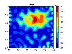
We employ the RNN method to solve the Poisson equation (1) with the exact solution $u=\sin(2\pi x)\sin(2\pi y)$ . The absolute error of the RNN method is plotted in Fig. 2.

It is observed that the error of the RNN method concentrates around the boundary $\partial\Omega$ . To improve the accuracy of the RNN method, it is necessary to approximate more accurately around the boundary.

2.3 RNN-Scaling method

To get a more accurate approximation around the boundary, a straightforward idea is to select a larger $N_{b}$ , would require placing more collocation points on on $\partial\Omega$ . However, this may increase the computational cost, and the improvement is not significant. Therefore, we slightly adjust the algebraic equations (2), to enlarge the weight of boundary equations.

We present the RNN-Scaling method with an example on the square domain. Let the number of collocation points on both the interior and boundary in both $x$ -direction and $y$ -direction be the same, denoted as $N$ . It is obvious that $N_{f}=N^{2}$ and $N_{f}=4N$ . The corresponding equations of the RNN-Scaling method are modified to

	$\displaystyle\frac{1}{N^{2}}\sum_{j=1}^{M}\omega_{j}L\varphi_{j}(\mathbf{x}_{f}^{i})$	$\displaystyle=\frac{1}{N^{2}}f(\mathbf{x}^{i}_{f}),$	$\displaystyle i=1,\cdots,N_{f},$		(3)
	$\displaystyle\sum_{j=1}^{M}\omega_{j}\varphi_{j}(\mathbf{x}_{b}^{i})$	$\displaystyle=g(\mathbf{x}_{b}^{i}),$	$\displaystyle i=1,\cdots,N_{b}.$		(3)

Solving the system (3) of equations yields the solution $\hat{u}({\mathbf{x}})$ .

We present the absolute error of the RNN-Scaling method in Fig. 3 and observe that the error of the RNN-Scaling method is much reduced around the boundary $\partial\Omega$ . Consequently, the total relative $L^{2}$ error is also reduced by about $10^{3}$ orders of magnitude.

Remark 1.

The weight coefficient $\frac{1}{N^{2}}$ is selected intuitively and numerically. In the classical methods, such as the finite element methods and the finite difference methods, the scale of the equations for interior unknowns is usually larger than that of the boundary unknowns by about $\frac{1}{N^{2}}$ magnitude. We test several numerical examples and find that $\frac{1}{N^{2}}$ seems to be a proper selection for the Poisson equation.

Remark 2.

The idea of the RNN-Scaling could be extended to a general domain. For instance, on a unit circular domain if we take $h=\frac{1}{N}$ as the “mesh size”, i.e., the average distance of collocation points. Then the interior collocation points could be the uniformly distributed points in the unit disk at a distance of $h$ , and the boundary collocation points could be $[2\pi N]$ uniformly distributed points on the circle. The distribution of collocation points on the unit circle is illustrated in Fig. 7(a). The weight coefficient is also selected to be $\frac{1}{N^{2}}$ . In this case, the total relative $L^{2}$ error is also reduced by 1-2 orders of magnitude.

2.4 RNN-BP method

As shown in Fig. 3, although the error of the RNN-Scaling method has decreased significantly, it still exists on the boundary $\partial\Omega$ . In this subsection, we propose a boundary processing technique that enforces the exact Dirichlet boundary condition. This boundary processing technique was also proposed in [12]. The advantage of boundary processing is that the boundary condition is imposed on the numerical solution over the entire boundary, rather than just at collocation points. We now describe the construction of the RNN-BP method. For simplicity, we consider the unit square domain $\Omega=(0,1)\times(0,1)$ and denote ${\mathbf{x}}$ as $(x,y)$ . It should be noted that the technique can be easily extended to rectangular domains.

We construct the numerical solution of the RNN-BP method as follows:

\displaystyle\begin{aligned} \hat{u}(x,y)=B(x,y)\sum_{j=1}^{M}\omega_{j}\varphi_{j}(x,y)+g_{D}(x,y),\end{aligned}

(4)

where $B$ and $g_{D}$ should satisfy

\displaystyle\begin{aligned} B(x,y)&=0,\quad&&\text{on~{}}\partial\Omega,\\ B(x,y)&\neq 0,\quad&&\text{in~{}}\Omega,\\ g_{D}(x,y)&=g(x,y),\quad&&\text{on~{}}\partial\Omega.\end{aligned}

A straightforward idea is to choose $B(x,y)=x(1-x)y(1-y)$ for the Poisson equation. The network architecture is illustrated in Fig. 4.

We next describe the construction of $g_{D}(x,y)$ . Let $g_{D}(x,y)=s(x,y)+P(x,y)$ . We construct $P(x,y)$ to satisfy the relations at four corners:

\displaystyle P(x_{i},y_{j})

\displaystyle=u(x_{i},y_{j}),

where $i,j=0,1$ and $x_{0}=y_{0}=0$ , $x_{1}=y_{1}=1$ . Rewrite the Dirichlet boundary condition to

\displaystyle\begin{aligned} &u(0,y)=t_{1}(y),\quad 0\leq y\leq 1,\\ &u(1,y)=t_{2}(y),\quad 0\leq y\leq 1,\\ &u(x,0)=t_{3}(x),\quad 0\leq x\leq 1,\\ &u(x,1)=t_{4}(x),\quad 0\leq x\leq 1.\end{aligned}

By using one-dimensional two-point Lagrange interpolation functions $l_{0}(x)=1-x$ and $l_{1}(x)=x$ , $P(x,y)$ can be expressed as a bilinear Lagrange interpolation function:

P(x,y)=\left[\begin{array}[]{c}l_{0}(x)\\ l_{1}(x)\end{array}\right]^{\mathrm{T}}\left[\begin{array}[]{ll}u(x_{0},y_{0})&u(x_{0},y_{1})\\ u(x_{1},y_{0})&u(x_{1},y_{1})\end{array}\right]\left[\begin{array}[]{c}l_{0}(y)\\ l_{1}(y)\\ \end{array}\right],

or equivalently,

P(x,y)=\left[\begin{array}[]{c}l_{0}(x)\\ l_{1}(x)\end{array}\right]^{\mathrm{T}}\left[\begin{array}[]{llll}t_{1}(y_{0})&t_{1}(y_{1})\\ t_{2}(y_{0})&t_{2}(y_{1})\end{array}\right]\left[\begin{array}[]{c}l_{0}(y)\\ l_{1}(y)\end{array}\right].

Denote $\tilde{u}(x,y)\triangleq u(x,y)-P(x,y)$ . Then, we construct $s(x,y)$ to satisfy the Dirichlet condition of $\tilde{u}$ exactly, i.e.,

\displaystyle s(x,y)=\tilde{u}(x,y),\quad\text{on }\partial\Omega.

The boundary conditions of $\tilde{u}(x,y)$ are denoted by $\tilde{t}_{i}$ , and there hold

\displaystyle\begin{aligned} &\tilde{t}_{1}(y)=t_{1}(y)-P(0,y),\quad 0\leq y\leq 1,\\ &\tilde{t}_{2}(y)=t_{2}(y)-P(1,y),\quad 0\leq y\leq 1,\\ &\tilde{t}_{3}(x)=t_{3}(x)-P(x,0),\quad 0\leq x\leq 1,\\ &\tilde{t}_{4}(x)=t_{4}(x)-P(x,1),\quad 0\leq x\leq 1.\end{aligned}

We define $s(x,y)$ as

\displaystyle\begin{aligned} s(x,y)&=l_{0}(x)\tilde{t}_{1}(y)+l_{1}(x)\tilde{t}_{2}(y)+l_{0}(y)\tilde{t}_{3}(x)+l_{1}(y)\tilde{t}_{4}(x).\end{aligned}

After constructing $s(x,y)$ and $P(x,y)$ , the corresponding equations of the RNN-BP method are derived as follows.

\displaystyle-\sum_{j=1}^{M}\omega_{j}\Delta(B\varphi_{j})(\mathbf{x}_{f}^{i})

\displaystyle=f(\mathbf{x}^{i}_{f})+\Delta s({\mathbf{x}}_{f}^{i})+\Delta P({\mathbf{x}}_{f}^{i}),

\displaystyle i=1,\cdots,N_{f}.

(5)

Theorem 1.

The numerical solution (4) of the RNN-BP method satisfies the Dirichlet boundary condition exactly.

Proof.

Our aim is to prove that $\hat{u}(x,y)-P(x,y)=\tilde{u}(x,y)$ on $\partial\Omega$ , i.e., $\sum_{i=1}^{M}\omega_{i}x(1-x)y(1-y)\varphi_{i}(x,y)+s(x,y)=\tilde{u}(x,y)$ on $\partial\Omega$ . Notice that $\sum_{i=1}^{M}\omega_{i}x(1-x)y(1-y)\varphi_{i}(x,y)$ satisfies the homogeneous Dirichlet boundary condition, thus we just need to prove that $s(0,y)=\tilde{t}_{1}(y)$ . It follows that

	$\displaystyle s(0,y)$	$\displaystyle=l_{0}(0)\tilde{t}_{1}(y)+l_{1}(0)\tilde{t}_{2}(y)+l_{0}(y)\tilde{t}_{3}(0)+l_{1}(y)\tilde{t}_{4}(0)$
		$\displaystyle=\tilde{t}_{1}(y),$

where we use the fact that $\tilde{t}_{i}(0)=\tilde{t}_{i}(1)=0$ for $i=1,\cdots,4.$

The conditions on the other boundary can be proved similarly. It completes the proof. ∎

Theorem 2.

Assume that the solution to the least squares problem (5) is uniquely solvable. Then the RNN-BP method is exact for solutions of the form

f_{1}(x)p_{1}(y)+f_{2}(y)p_{2}(x),

(6)

where $f_{1},f_{2}\in C(\Omega)$ , $p_{1}$ and $p_{2}$ are polynomials of degree no higher than 1.

Proof.

For simplicity, we only provide the proof for the case where $u(x,y)=f_{1}(x)p_{1}(y)$ . The proof for for the case where $u(x,y)=f_{1}(x)p_{1}(y)+f_{2}(y)p_{2}(x)$ is similar and thus is omitted.

The first step is to prove that $u(x,y)=s(x,y)$ under the assumption that $u(x,y)=0$ at the four corner points of $\partial\Omega$ . It is obvious $P(x,y)\equiv 0$ from the above assumption. We analyze the four terms of $s(x,y)=l_{0}(x)t_{1}(y)+l_{1}(x)t_{2}(y)+l_{0}(y)t_{3}(x)+l_{1}(y)t_{4}(x)$ sequentially. For the term $t_{1}(y)=f_{1}(0)p_{1}(y)\in\mathbb{P}_{1}$ , we have $t_{1}(0)=t_{1}(1)=0$ . Consequently, $t_{1}(y)\equiv 0$ in $[0,1]$ . Similarly, we have $t_{2}(y)\equiv 0$ in $[0,1]$ . Hence we obtain

	$\displaystyle s(x,y)$	$\displaystyle=l_{0}(x)t_{1}(y)+l_{1}(x)t_{2}(y)+l_{0}(y)t_{3}(x)+l_{1}(y)t_{4}(x)$
		$\displaystyle=l_{0}(y)f_{1}(x)p_{1}(0)+l_{1}(y)f_{1}(x)p_{1}(1)$
		$\displaystyle=f_{1}(x)(l_{0}(y)p_{1}(0)+l_{1}(y)p_{1}(1))$
		$\displaystyle=f_{1}(x)p_{1}(y).$

The second step is to prove that $u(x,y)=s(x,y)+P(x,y)$ when $u(x,y)=f_{1}(x)p_{1}(y)$ . Define $Q(x)$ as a first-order polynomial that satisfies $Q(0)=f_{1}(0)$ and $Q(1)=f_{1}(1)$ . From the definition of $P(x,y)$ and $Q(x)p_{1}(y)=P(x,y)$ at four corners of $\partial\Omega$ , it follows that $Q(x)p_{1}(y)\equiv P(x,y)$ . Thus, it yields that

	$\displaystyle u(x,y)-P(x,y)$	$\displaystyle=(f_{1}(x)-Q(x))p_{1}(y)$		(7)
		$\displaystyle=s(x,y),$		(7)

for any $(x,y)\in\Omega$ , where the final equation adopts the conclusion of the first step since $f_{1}(x)-Q(x)=0$ at four corners of $\partial\Omega$ . Substituting (7) into (5) yields that $\sum_{j=1}^{M}\omega_{j}\Delta(B({\mathbf{x}}_{f}^{i})\varphi_{j}({\mathbf{x}}_{f}^{i}))=0$ for $i=1,\cdots,N_{f}$ , then it is obvious that $\{\omega_{j}\}_{j=1}^{M}=0$ is a solution to the least squares problem. Hence, we obtain

\hat{u}(x,y)=u(x,y),\quad\text{in~{}}\Omega,

which completes the proof. ∎

3 The improved RNN methods for the biharmonic equation

In this section, we focus on the biharmonic equation with clamped boundary condition on the bounded domain with boundary $\partial\Omega$ :

\displaystyle\left\{\begin{aligned} \Delta^{2}u({\mathbf{x}})&=f({\mathbf{x}}),&\text{in }&\Omega,\\ u({\mathbf{x}})&=g_{1}({\mathbf{x}}),&\text{on }&\partial\Omega,\\ \frac{\partial u}{\partial\mathbf{n}}({\mathbf{x}})&=g_{2}({\mathbf{x}}),&\text{on }&\partial\Omega.\end{aligned}\right.

(8)

The source term $f({\mathbf{x}})$ and the boundary conditions $g_{1}({\mathbf{x}})$ and $g_{2}({\mathbf{x}})$ are given functions, $\mathbf{n}$ denotes the unit outward normal vector of $\partial\Omega$ .

3.1 RNN method and RNN-Scaling method

For the biharmonic equation, the equations of the RNN method are

$\displaystyle\sum_{j=1}^{M}\omega_{j}\Delta^{2}\varphi_{j}(\mathbf{x}_{f}^{i})$	$\displaystyle=f(\mathbf{x}^{i}_{f}),$	$\displaystyle i=1,\cdots,N_{f},$
$\displaystyle\sum_{j=1}^{M}\omega_{j}\varphi_{j}(\mathbf{x}_{b}^{i})$	$\displaystyle=g_{1}(\mathbf{x}_{b}^{i}),$	$\displaystyle i=1,\cdots,N_{b},$
$\displaystyle\sum_{j=1}^{M}\omega_{j}\frac{\partial\varphi_{j}}{\partial{\mathbf{n}}}(\mathbf{x}_{b}^{i})$	$\displaystyle=g_{2}(\mathbf{x}^{i}_{b}),$	$\displaystyle i=1,\cdots,N_{b},$

where $N_{f}$ and $N_{b}$ still represent the numbers of interior and boundary collocation points, respectively. Solving this system of equations yields $\omega$ , which consequently obtains the solution $\hat{u}({\mathbf{x}})$ .

For the biharmonic equation, we also observe that the error of the RNN method is concentrated around the boundary. Therefore, similar to the Poisson equation, it is necessary to develop an improved method to reduce the error around the boundary.

We describe the RNN-Scaling method on the square domain. Let the numbers of collocation points on both interior and boundary in the $x$ -direction and $y$ -direction be the same, still denoted as $N$ , then $N_{f}=N^{2}$ and $N_{b}=4N$ . The least squares problem is then adjusted to

$\displaystyle\frac{1}{N^{4}}\sum_{j=1}^{M}\omega_{j}\Delta^{2}\varphi_{j}(\mathbf{x}_{f}^{i})$	$\displaystyle=\frac{1}{N^{4}}f(\mathbf{x}^{i}_{f}),$	$\displaystyle i=1,\cdots,N_{f},$	(9)
$\displaystyle\sum_{j=1}^{M}\omega_{j}\varphi_{j}(\mathbf{x}_{b}^{i})$	$\displaystyle=g_{1}(\mathbf{x}_{b}^{i}),$	$\displaystyle i=1,\cdots,N_{b},$
$\displaystyle\frac{1}{N}\sum_{j=1}^{M}\omega_{j}\frac{\partial\varphi_{j}}{\partial{\mathbf{n}}}(\mathbf{x}_{b}^{i})$	$\displaystyle=\frac{1}{N}g_{2}(\mathbf{x}^{i}_{f}),$	$\displaystyle i=1,\cdots,N_{b}.$

Solving the system (9) obtains the numerical solution $\hat{u}({\mathbf{x}})$ .

Remark 3.

The idea of the RNN-Scaling could also be extended to general domain for the biharmonic equation. For instance, on a unit circular domain, if we take $h=\frac{1}{N}$ as the “mesh size”, then the interior collocation points could be the uniformly distributed points in the unit disk at a distance of $h$ , and the boundary collocation points could be $[2\pi N]$ uniformly distributed points on the circle. The weight coefficients are also chosen to be $\frac{1}{N^{4}}$ and $\frac{1}{N}$ . The total relative $L^{2}$ error is also reduced by 1-2 orders of magnitude.

3.2 RNN-BP method

We observe that the error of the RNN-Scaling method is reduced significantly, but still exists on the boundary. Therefore, we enforce the neural network to satisfy the exact clamped boundary condition on the square domain.

The neural network of RNN-BP method for the biharmonic equation is

\displaystyle\begin{aligned} \hat{u}(x,y)=B(x,y)\sum_{i=1}^{M}\omega_{i}\varphi_{i}(x,y)+g_{D}(x,y),\end{aligned}

(10)

where $B(x,y)$ and $g_{D}(x,y)$ should satisfy the following conditions:

$\displaystyle B(x,y)$	$\displaystyle=0,\quad$	$\displaystyle\text{on~{}}\partial\Omega,$
$\displaystyle\frac{\partial B}{\partial{\mathbf{n}}}(x,y)$	$\displaystyle=0,\quad$	$\displaystyle\text{on~{}}\partial\Omega,$
$\displaystyle B(x,y)$	$\displaystyle\neq 0,\quad$	$\displaystyle\text{in~{}}\Omega,$
$\displaystyle g_{D}(x,y)$	$\displaystyle=g_{1}(x,y),\quad$	$\displaystyle\text{on~{}}\partial\Omega,$
$\displaystyle\frac{\partial{g_{D}}}{\partial{\mathbf{n}}}(x,y)$	$\displaystyle=g_{2}(x,y),\quad$	$\displaystyle\text{on~{}}\partial\Omega.$

For the biharmonic equation, we define $B(x,y)=x^{2}(1-x)^{2}y^{2}(1-y)^{2}$ .

Next, we provide the construction of $g_{D}(x,y)$ . Let $g_{D}(x,y)=s(x,y)+P(x,y)$ . We construct $P(x,y)$ to satisfy the following relations at four corners:

	$\displaystyle P(x_{i},y_{j})$	$\displaystyle=u(x_{i},y_{j}),$
	$\displaystyle P_{x}(x_{i},y_{j})$	$\displaystyle=u_{x}(x_{i},y_{j}),$
	$\displaystyle P_{y}(x_{i},y_{j})$	$\displaystyle=u_{y}(x_{i},y_{j}),$
	$\displaystyle P_{xy}(x_{i},y_{j})$	$\displaystyle=u_{xy}(x_{i},y_{j}),$

where $i,j=0,1$ , $x_{0}=y_{0}=0$ , $x_{1}=y_{1}=1$ . Rewrite the clamped boundary condition (8) to

\displaystyle\begin{aligned} &u(0,y)=t_{1}(y),\quad\frac{\partial u}{\partial x}(0,y)=h_{1}(y),\quad 0\leq y\leq 1,\\ &u(1,y)=t_{2}(y),\quad\frac{\partial u}{\partial x}(1,y)=h_{2}(y),\quad 0\leq y\leq 1,\\ &u(x,0)=t_{3}(x),\quad\frac{\partial u}{\partial y}(x,0)=h_{3}(x),\quad 0\leq x\leq 1,\\ &u(x,1)=t_{4}(x),\quad\frac{\partial u}{\partial y}(x,1)=h_{4}(x),\quad 0\leq x\leq 1.\end{aligned}

Recall the two-point Hermite interpolation basis functions

		$\displaystyle H_{i}(x)=l_{i}^{2}(x)\left(1-2l_{i}^{\prime}\left(x_{i}\right)\left(x-x_{i}\right)\right),$
		$\displaystyle G_{i}(x)=l_{i}^{2}(x)\left(x-x_{i}\right),$

for $i=0,1$ , where $l_{0}(x)$ and $l_{1}(x)$ are the first-order Lagrange interpolation functions. We present $P(x,y)$ with the following expression:

P(x,y)=\left[\begin{array}[]{c}H_{0}(x)\\ H_{1}(x)\\ G_{0}(x)\\ G_{1}(x)\end{array}\right]^{\mathrm{T}}\left[\begin{array}[]{llll}u(x_{0},y_{0})&u(x_{0},y_{1})&u_{y}(x_{0},y_{0})&u_{y}(x_{0},y_{1})\\ u(x_{1},y_{0})&u(x_{1},y_{1})&u_{y}(x_{1},y_{0})&u_{y}(x_{1},y_{1})\\ u_{x}(x_{0},y_{0})&u_{x}(x_{0},y_{1})&u_{xy}(x_{0},y_{0})&u_{xy}(x_{0},y_{1})\\ u_{x}(x_{1},y_{0})&u_{x}(x_{1},y_{1})&u_{xy}(x_{1},y_{0})&u_{xy}(x_{1},y_{1})\end{array}\right]\left[\begin{array}[]{c}H_{0}(y)\\ H_{1}(y)\\ G_{0}(y)\\ G_{1}(y)\end{array}\right].

Alternatively, the expression for $P(x,y)$ can be written as

P(x,y)=\left[\begin{array}[]{c}H_{0}(x)\\ H_{1}(x)\\ G_{0}(x)\\ G_{1}(x)\end{array}\right]^{\mathrm{T}}\left[\begin{array}[]{llll}t_{1}(y_{0})&t_{1}(y_{1})&h_{3}(x_{0})&h_{4}(x_{0})\\ t_{2}(y_{0})&t_{2}(y_{1})&h_{3}(x_{1})&h_{4}(x_{1})\\ h_{1}(y_{0})&h_{1}(y_{1})&h_{3}^{\prime}(x_{0})&h_{4}^{\prime}(x_{0})\\ h_{2}(y_{0})&h_{2}(y_{1})&h_{3}^{\prime}(x_{1})&h_{4}^{\prime}(x_{1})\end{array}\right]\left[\begin{array}[]{c}H_{0}(y)\\ H_{1}(y)\\ G_{0}(y)\\ G_{1}(y)\end{array}\right].

Then, we construct $s(x,y)$ to satisfy the clamped condition of $\tilde{u}(x,y)$ , where $\tilde{u}(x,y)\triangleq u(x,y)-P(x,y)$ .

\displaystyle\left\{\begin{aligned} s(x,y)&=\tilde{u}(x,y),&\text{on }&\partial\Omega,\\ \frac{\partial s}{\partial\mathbf{n}}(x,y)&=\frac{\partial\tilde{u}}{\partial\mathbf{n}}(x,y),&\text{on }&\partial\Omega.\end{aligned}\right.

The boundary functions of $\tilde{u}(x,y)$ are denoted by $\tilde{t}_{i}$ and $\tilde{h}_{i}$ , and there hold

\displaystyle\begin{aligned} &\tilde{t}_{1}(y)=t_{1}(y)-P(0,y),\quad\tilde{h}_{1}(y)=h_{1}(y)-\frac{\partial P}{\partial x}(0,y),\quad 0\leq y\leq 1,\\ &\tilde{t}_{2}(y)=t_{2}(y)-P(1,y),\quad\tilde{h}_{2}(y)=h_{2}(y)-\frac{\partial P}{\partial x}(1,y),\quad 0\leq y\leq 1,\\ &\tilde{t}_{3}(x)=t_{3}(x)-P(x,0),\quad\tilde{h}_{3}(x)=h_{3}(x)-\frac{\partial P}{\partial y}(x,0),\quad 0\leq x\leq 1,\\ &\tilde{t}_{4}(x)=t_{4}(x)-P(x,1),\quad\tilde{h}_{4}(x)=h_{4}(x)-\frac{\partial P}{\partial y}(x,1),\quad 0\leq x\leq 1.&\end{aligned}

Define $s(x,y)$ as

\displaystyle\begin{aligned} s(x,y)&=H_{0}(x)\tilde{t}_{1}(y)+H_{1}(x)\tilde{t}_{2}(y)+H_{0}(y)\tilde{t}_{3}(x)+H_{1}(y)\tilde{t}_{4}(x)\\ &+G_{0}(x)\tilde{h}_{1}(y)+G_{1}(x)\tilde{h}_{2}(y)+G_{0}(y)\tilde{h}_{3}(x)+G_{1}(y)\tilde{h}_{4}(x).\end{aligned}

Finally, the corresponding equations for the RNN-BP method are

\displaystyle\sum_{j=1}^{M}\omega_{j}\Delta^{2}(B\varphi_{j})(\mathbf{x}_{f}^{i})

\displaystyle=f(\mathbf{x}^{i}_{f})-\Delta^{2}s({\mathbf{x}}_{f}^{i})-\Delta^{2}P({\mathbf{x}}_{f}^{i}),

\displaystyle i=1,\cdots,N_{f}.

(11)

We emphasize that the clamped boundary condition can be exactly imposed. This boundary processing method on rectangular domains is applicable to any PDEs with the clamped boundary condition.

Theorem 3.

The numerical solution (10) of the RNN-BP method satisfies the clamped boundary condition of (8) exactly.

Proof.

If we can prove that $\hat{u}(x,y)-P(x,y)=\sum_{i=1}^{M}\omega_{i}B(x,y)\varphi_{i}(x,y)+s(x,y)$ satisfies the clamped boundary condition of $\tilde{u}(x,y)$ , then the theorem follows immediately. Since $P(x,y)$ is the cubic Hermit interpolation of $u(x,y)$ on $\bar{\Omega}$ , there hold

\displaystyle\begin{aligned} &\tilde{t}_{i}(0)=\tilde{h}_{i}(0)=\tilde{h}_{i}^{\prime}(0)=0,\\ &\tilde{t}_{i}(1)=\tilde{h}_{i}(1)=\tilde{h}_{i}^{\prime}(1)=0,\end{aligned}

(12)

for $i=1,\cdots,4$ .

It is easy to check that $\sum_{i=1}^{M}\omega_{i}x^{2}(1-x)^{2}y^{2}(1-y)^{2}\varphi_{i}(x,y)$ satisfies the homogeneous clamped boundary condition, so we need to prove that $s(0,y)=\tilde{t}_{1}(y),\dfrac{\partial s}{\partial x}(0,y)=\tilde{h}_{1}(y)$ . It follows from (LABEL:prove1) that

	$\displaystyle s(0,y)$	$\displaystyle=H_{0}(0)\tilde{t}_{1}(y)+H_{1}(0)\tilde{t}_{2}(y)+H_{0}(y)\tilde{t}_{3}(0)+H_{1}(y)\tilde{t}_{4}(0)$
		$\displaystyle+G_{0}(0)\tilde{h}_{1}(y)+G_{1}(0)\tilde{h}_{2}(y)+G_{0}(y)\tilde{h}_{3}(0)+G_{1}(y)\tilde{h}_{4}(0)$
		$\displaystyle=\tilde{t}_{1}(y),$
	$\displaystyle\frac{\partial s}{\partial x}(0,y)$	$\displaystyle=H_{0}^{\prime}(0)\tilde{t}_{1}(y)+H_{1}^{\prime}(0)\tilde{t}_{2}(y)+H_{0}(y)\tilde{t}_{3}^{\prime}(0)+H_{1}(y)\tilde{t}_{4}^{\prime}(0)$
		$\displaystyle+G_{0}^{\prime}(0)\tilde{h}_{1}(y)+G_{1}^{\prime}(0)\tilde{h}_{2}(y)+G_{0}(y)\tilde{h}_{3}^{\prime}(0)+G_{1}(y)\tilde{h}_{4}^{\prime}(0)$
		$\displaystyle=\tilde{h}_{1}(y).$

The clamped conditions on the other boundary can be proved similarly. It completes the proof. ∎

Theorem 4.

Assume that the solution to the least squares problem (11) is uniquely solvable. Then the RNN-BP method is exact for solutions of the form

f_{1}(x)p_{1}(y)+f_{2}(y)p_{2}(x),

(13)

where $f_{1},f_{2}\in C^{1}(\Omega)$ , $p_{1}$ and $p_{2}$ are polynomials of degree no higher than 3.

Proof.

The proof of this theorem is similar to that of Theorem 2, but for completeness, we still provide the proof. We still only provide the proof for the case where $u(x,y)=f_{1}(x)p_{1}(y)$ .

We also divide our proof into two steps. The first step is to prove that $u(x,y)=s(x,y)$ under the assumption that $u(x,y)=0$ and $\dfrac{\partial u}{\partial{\mathbf{n}}}(x,y)=0$ at the four corner points of $\partial\Omega$ . It is obvious $P(x,y)\equiv 0$ from the above assumption. We analyze the eight terms of $s(x,y)$ sequentially. Similar to the proof of Theorem 2, we have $t_{1}(y)=t_{2}(y)=h_{1}(y)=h_{2}(y)=0$ in $[0,1]$ . Then it follows that

	$\displaystyle s(x,y)$	$\displaystyle=H_{0}(y)t_{3}(x)+H_{1}(y)t_{4}(x)+G_{0}(y)h_{3}(x)+G_{1}(y)h_{4}(x)$
		$\displaystyle=f_{1}(x)(H_{0}(y)p_{1}(0)+H_{1}(y)p_{1}(1)-G_{0}(y)p^{\prime}_{1}(0)+G_{1}(y)p^{\prime}_{1}(1))$
		$\displaystyle=f_{1}(x)p_{1}(y).$

The second step is to prove that $u(x,y)=s(x,y)+P(x,y)$ when $u(x,y)=f_{1}(x)p_{1}(y)$ . Define $Q(x)$ as a first-order polynomial such that $Q(0)=f_{1}(0)$ , $Q(1)=f_{1}(1)$ , $Q(0)=-f^{\prime}_{1}(0)$ and $Q(1)=f^{\prime}_{1}(1)$ . From the definition of $P(x,y)$ , it can be inferred that $Q(x)p_{1}(y)\equiv P(x,y)$ on $\Omega$ . It yields that

	$\displaystyle u(x,y)-P(x,y)$	$\displaystyle=(f_{1}(x)-Q(x))p_{1}(y)$		(14)
		$\displaystyle=s(x,y),$		(14)

for any $(x,y)\in\Omega$ , where the final equation of (14) adopts the conclusion of the first step. Substituting (14) into (11) yields that $\sum_{j=1}^{M}\omega_{j}\Delta(B({\mathbf{x}}_{f}^{i})\varphi_{j}({\mathbf{x}}_{f}^{i}))=0$ for $i=1,\cdots,N_{f}$ , which implies that $\{\omega_{j}\}_{j=1}^{M}=0$ is a solution to the least squares problem. Hence, we obtain

\displaystyle\begin{aligned} \hat{u}(x,y)=u(x,y),\quad\text{in~{}}\Omega.\end{aligned}

It completes the proof. ∎

4 Numerical experiments

In the numerical experiments, we compare the performance of the three methods by using relative $L^{2}$ error

\|e\|_{L^{2}}=\frac{\sqrt{\sum_{i=1}^{N_{test}}\left|\hat{u}({\mathbf{x}}_{i})-u({\mathbf{x}}_{i})\right|^{2}}}{\sqrt{\sum_{i=1}^{N_{test}}\left|u({\mathbf{x}}_{i})\right|^{2}}},

where $N_{test}$ denotes the number of uniform collocation points in $\bar{\Omega}$ and we set $N_{test}=10^{4}$ for all examples. Throughout this paper, we employ Sin function as the activation function. In all tables, we abbreviate RNN-Scaling as RNN-S for simplicity.

4.1 Poisson equation

First, we test our methods for the Poisson equation.

4.1.1 Example 1.1

In the first example, we consider the exact solution on $\Omega=(0,1)\times(0,1)$ :

u(x,y)=\sin 2\pi x\sin 2\pi y.

The numbers of points in $x$ and $y$ dimensions are set to be the same, which are denoted as $N$ . We employ a neural network containing 2 hidden layers with 100 and $M$ neurons, respectively. We compare the relative $L^{2}$ errors of the RNN, RNN-Scaling, and RNN-BP methods across varying different numbers of collocation points and $M$ . Tables 1 and 2 present the comparison results between the default and uniform random initialization $R_{m}=1$ , respectively.

Table 1: Comparison of three methods with the default initialization for Example 1.1.

method	$N$	$M$	50	100	150	200	250	300	400	500
RNN	8	$\\|e\\|_{L^{2}}$	9.44e-1	2.76e-3	1.01e-3	4.82e-4	7.79e-4	5.49e-4	4.49e-4	3.66e-4
	12	$\\|e\\|_{L^{2}}$	9.15e-1	3.13e-4	1.11e-6	3.99e-7	1.83e-7	8.14e-7	2.53e-7	5.97e-7
	16	$\\|e\\|_{L^{2}}$	9.45e-1	6.63e-4	2.43e-6	2.66e-7	1.35e-7	4.53e-8	2.67e-7	1.16e-7
	24	$\\|e\\|_{L^{2}}$	1.04e+0	9.26e-4	3.61e-6	1.33e-6	2.06e-7	1.76e-7	1.46e-7	1.41e-7
	32	$\\|e\\|_{L^{2}}$	1.14e+0	1.04e-3	3.99e-6	2.51e-6	2.84e-7	1.87e-7	1.27e-6	2.83e-7
	48	$\\|e\\|_{L^{2}}$	1.34e+0	1.20e-3	4.40e-6	2.35e-6	1.13e-6	1.94e-6	1.65e-6	1.08e-6
RNN-S	8	$\\|e\\|_{L^{2}}$	2.09e-2	2.76e-3	1.01e-3	4.82e-4	7.79e-4	5.49e-4	3.06e-4	3.66e-4
	12	$\\|e\\|_{L^{2}}$	1.75e-2	2.04e-5	4.35e-7	2.18e-7	3.04e-7	3.38e-7	6.22e-7	5.11e-7
	16	$\\|e\\|_{L^{2}}$	1.57e-2	1.42e-5	9.53e-8	8.78e-8	1.08e-7	2.19e-8	1.65e-7	2.60e-8
	24	$\\|e\\|_{L^{2}}$	1.43e-2	1.31e-5	1.75e-7	3.29e-7	5.43e-8	8.21e-8	2.56e-7	3.32e-8
	32	$\\|e\\|_{L^{2}}$	1.41e-2	1.29e-5	3.67e-7	3.42e-7	1.63e-7	8.12e-8	2.43e-7	5.47e-8
	48	$\\|e\\|_{L^{2}}$	1.48e-2	1.27e-5	3.31e-6	1.26e-6	1.37e-6	3.31e-6	2.18e-6	2.27e-7
RNN-BP	8	$\\|e\\|_{L^{2}}$	3.55e-4	3.42e-4	1.89e-4	2.43e-4	1.01e-4	1.02e-4	1.64e-4	8.70e-5
	12	$\\|e\\|_{L^{2}}$	1.09e-4	2.37e-7	7.55e-8	5.59e-8	4.99e-8	7.74e-8	4.37e-8	7.58e-8
	16	$\\|e\\|_{L^{2}}$	1.05e-4	3.72e-8	7.54e-10	4.63e-10	6.68e-10	8.87e-11	6.72e-10	3.61e-10
	24	$\\|e\\|_{L^{2}}$	1.02e-4	2.30e-8	1.03e-10	1.20e-10	3.86e-10	1.13e-10	1.57e-10	3.86e-11
	32	$\\|e\\|_{L^{2}}$	9.89e-5	2.24e-8	1.63e-10	1.29e-10	2.36e-10	2.66e-10	2.74e-10	1.17e-10
	48	$\\|e\\|_{L^{2}}$	9.40e-5	2.13e-8	3.53e-10	5.00e-10	1.81e-10	1.37e-10	4.14e-10	4.34e-11

Table 2: Comparison of three methods with uniform random initialization (

R_{m}=1

) for Example 1.1.

method	$N$	$M$	50	100	150	200	250	300	400	500
RNN	8	$\\|e\\|_{L^{2}}$	2.19e+0	7.02e-3	4.37e-3	3.77e-3	2.89e-3	2.84e-3	4.05e-3	2.71e-3
	12	$\\|e\\|_{L^{2}}$	2.28e+0	5.55e-2	4.95e-4	1.32e-4	3.07e-5	2.36e-5	2.79e-5	2.35e-5
	16	$\\|e\\|_{L^{2}}$	2.47e+0	6.08e-2	1.88e-3	3.34e-5	7.44e-7	9.90e-7	1.22e-7	2.34e-7
	24	$\\|e\\|_{L^{2}}$	2.73e+0	6.30e-2	2.46e-3	8.14e-5	3.02e-6	1.15e-7	2.86e-10	4.17e-11
	32	$\\|e\\|_{L^{2}}$	2.94e+0	6.48e-2	2.73e-3	9.64e-5	3.61e-6	1.78e-7	9.82e-10	3.54e-11
	48	$\\|e\\|_{L^{2}}$	3.25e+0	6.83e-2	3.05e-3	1.11e-4	4.24e-6	2.06e-7	1.62e-9	1.24e-10
RNN-S	8	$\\|e\\|_{L^{2}}$	9.25e-2	7.02e-3	4.37e-3	3.77e-3	2.89e-3	2.84e-3	4.05e-3	2.71e-3
	12	$\\|e\\|_{L^{2}}$	8.07e-2	6.80e-4	4.51e-5	1.32e-4	3.07e-5	2.36e-5	2.79e-5	2.35e-5
	16	$\\|e\\|_{L^{2}}$	8.58e-2	5.73e-4	1.61e-5	8.15e-7	5.36e-7	3.49e-7	1.51e-7	2.34e-7
	24	$\\|e\\|_{L^{2}}$	9.02e-2	5.07e-4	1.22e-5	3.36e-7	1.87e-8	2.06e-9	1.42e-10	3.48e-11
	32	$\\|e\\|_{L^{2}}$	9.27e-2	5.00e-4	1.13e-5	3.01e-7	1.26e-8	5.67e-10	1.20e-11	2.69e-12
	48	$\\|e\\|_{L^{2}}$	9.85e-2	5.12e-4	1.08e-5	2.87e-7	1.24e-8	4.77e-10	5.73e-12	8.27e-13
RNN-BP	8	$\\|e\\|_{L^{2}}$	1.15e-2	1.01e-2	4.40e-3	3.90e-3	5.34e-3	6.46e-3	4.21e-3	4.61e-3
	12	$\\|e\\|_{L^{2}}$	7.21e-3	1.77e-4	4.44e-5	1.05e-4	1.20e-4	5.07e-5	1.26e-4	5.76e-5
	16	$\\|e\\|_{L^{2}}$	6.87e-3	5.64e-5	2.17e-6	6.42e-7	1.30e-6	3.11e-7	1.66e-7	5.13e-7
	24	$\\|e\\|_{L^{2}}$	6.43e-3	4.06e-5	4.01e-7	1.38e-8	2.18e-9	2.51e-10	2.45e-11	2.12e-11
	32	$\\|e\\|_{L^{2}}$	6.18e-3	3.85e-5	3.80e-7	8.44e-9	4.35e-10	4.56e-11	9.71e-13	3.72e-13
	48	$\\|e\\|_{L^{2}}$	5.91e-3	3.57e-5	3.82e-7	8.42e-9	3.63e-10	1.69e-11	8.15e-14	2.55e-14

From Tables 1 and 2, we conclude the following observations. The errors of all three methods show a trend of first decreasing and then stabilizing under both two initialization methods. The errors of the RNN-scaling method are smaller than the RNN method. Especially under uniform random initialization, the performance is more stable, and the errors gradually decrease as $N$ and $M$ increase. The RNN-BP method, under both initialization methods, achieves smallest among the three methods and these errors decrease as $N$ and $M$ increase.

Figs. 5(a)-(b) illustrate that the RNN-Scaling and RNN-BP methods tend to produce smaller $L^{2}$ errors than the RNN method, especially under uniform random initialization with $R_{m}=1$ . This indicates that these two methods are more robust to initialization conditions and may perform better in practice. Under uniform random initialization, the performance of the three methods is generally better than that under the default initialization condition.

We compare the three methods across varying values of $R_{m}$ , where we fix $M=300$ and $N=48$ , and vary $R_{m}$ from 0.1 to 2. From Fig. 5(c), it can be seen that as $R_{m}$ varies, the three methods exhibit a similar trend. Specifically, when $R_{m}$ is around 0.3 to 1.5, the errors of the three methods are relatively small; when $R_{m}>1.5$ , the errors increase rapidly. The RNN-BP method produces the smallest error among the three methods.

4.1.2 Example 1.2

The second numerical example considers the exact solution on $\Omega=(0,2)^{2}$ :

u(x,y)=-\left[2\cos\left(\frac{3}{2}\pi x+\frac{2\pi}{5}\right)+\frac{3}{2}\cos\left(3\pi x-\frac{\pi}{5}\right)\right]\left[2\cos\left(\frac{3}{2}\pi y+\frac{2\pi}{5}\right)+\frac{3}{2}\cos\left(3\pi y-\frac{\pi}{5}\right)\right].

We compare the three methods varying max magnitude of random coefficient with the fixed network [2, 100, 500, 1] and $N=96$ . The result is presented in Fig. 6(a). It is observed that the optimal value of $R_{m}\approx 1.2$ . The RNN-BP method achieves the smallest error among the three methods, with the smallest error reaching 4.75 $\times 10^{-10}$ . We compare the methods with varying values of $M$ , with fixed $R_{m}=1$ and $N=64$ . Fig. 6(b) illustrates that the errors of all three methods decrease as $M$ increases, and the RNN-BP method remains the one with the smallest error.

4.1.3 Example 1.3

This example aims to demonstrate that the RNN-BP method is exact for the solution of the form (6). We consider the exact solution on $\Omega=(0,1)\times(0,1)$ :

u(x,y)=x^{10}+y^{10}+x^{k}\sin y+y^{k}\cos x,

where $k$ is an integer.

We compare the three methods with different numbers of collocation points for $k=1$ and $k=2$ , using a fixed network [2, 100, 300, 1] and random initialization ( $R_{m}=1$ ). The results are presented in Table 3. For the RNN-BP method, it can be observed that the relative $L^{2}$ errors achieve machine precision when $k=1$ . This verifies that the RNN-BP method is exact for the solution of the form (6). The errors decrease rapidly as the numbers of collocation points increase when $k=2$ , with the smallest error about $10^{-14}$ . The relative $L^{2}$ errors of the RNN-Scaling method are at most 3 orders of magnitude smaller than those of the RNN method.

Table 3: Comparison of three methods with different

N

for Example 1.3.

$k$	$N$	4	12	20	28	36	44	52
1	RNN	8.17e-1	1.41e-4	2.44e-7	6.32e-7	8.23e-7	9.00e-7	9.43e-7
	RNN-S	8.17e-1	1.41e-4	3.55e-8	5.47e-9	3.67e-9	3.56e-9	3.60e-9
	RNN-BP	2.35e-16	2.60e-16	2.57e-16	2.19e-16	2.19e-16	2.19e-16	2.19e-16
2	RNN	1.05e+0	1.70e-4	2.92e-7	7.58e-7	9.87e-7	1.08e-6	1.13e-6
	RNN-S	1.05e+0	1.70e-4	4.25e-8	6.56e-9	4.39e-9	4.26e-9	4.30e-9
	RNN-BP	2.64e-2	1.15e-6	1.39e-11	8.14e-13	1.62e-13	9.64e-14	9.06e-14

4.1.4 Example 1.4

This example considers the exact solution

u(x,y)=x^{4}+y^{4}

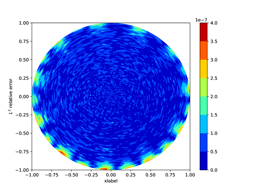
on the unit circle centered at $(0,0)$ .

We fix $N=64$ and vary $M$ to compare the RNN method and the RNN-Scaling method, where the network architecture is [2, 100, 100, $M$ , 1] and the default initialization method is employed. Fig. 7(a) shows an example of the uniform collocation points with $N=32$ . Fig. 7(b) presents the comparison results, it can be seen that the RNN-Scaling method produces the smallest error (about $10^{-9}$ ), and typically results in a reduction of 2 orders of magnitude in error compared to the RNN method. Figs. 7(c)-(d) illustrate the absolute errors of both methods when $N=64$ and $M=200$ , and it can be observed that the error of the RNN method is concentrated on the boundary, while the error of the RNN-Scaling method is concentrated in the interior.

From Examples 1.1-1.4, we offer the following summary for solving the Poisson equation. The RNN-BP method consistently achieves the smallest errors among the three methods. More specifically, when $M$ and $N$ are relatively large, the errors of the RNN-BP method are, on average, 4 orders of magnitude smaller than those of the RNN method in Example 1.1, and 3 orders of magnitude smaller than those of the RNN method in Example 1.2. Moreover, under both initialization methods, the errors of the RNN-BP method are significantly smaller than those of the other two methods, indicating that the RNN-BP method is more robust in practice.

On both the unit circular and square domains, the RNN-Scaling method is more accurate than the RNN method. Specifically, on the unit circular domain, the relative $L^{2}$ errors of the RNN-Scaling method are, on average, 2 orders of magnitude smaller than those of the RNN method. On the square domain, under the default initialization method, the errors of the RNN-Scaling method are, on average 2 orders of magnitude smaller than the RNN method when $M$ is small; and the difference between the two methods is not significant when $M$ is large. Under the uniform random initialization, the errors are, on average, 2 orders of magnitude smaller than those of the RNN method.

4.2 Biharmonic equation

Next, we test our methods for the biharmonic equation.

4.2.1 Example 2.1

In the first example, we consider the exact solution on $\Omega=(0,1)\times(0,1)$ :

u(x,y)=\sin\pi x\sin\pi y.

We employ a neural network containing 2 hidden layers with 100 and $M$ neurons, respectively. We compare the relative $L^{2}$ errors of the three methods with different numbers of collocation points and $M$ . Tables 4 and 5 present the comparison results with the default and uniform random initialization $R_{m}$ =1, respectively. Tables 4 and 5 demonstrate that the errors of all three methods significantly decrease as $M$ and $N$ increase. The RNN-BP method exhibits the best performance, followed by the RNN-Scaling method, and then the RNN method. Specifically, under the default initialization, the RNN-Scaling method results in a reduction of 1 to 4 orders of magnitude in error, and the RNN-BP method results in a reduction of 6 to 9 orders of magnitude in error. The RNN-BP method achieves machine precision when $M\geq 150$ and $N\geq 16$ . Under random initialization, the RNN-Scaling method achieves a reduction of up to 5 orders of magnitude in error, while the RNN-BP method results in a reduction of up to 7 orders of magnitude. These indicate that the RNN-BP and RNN-Scaling methods have a clear advantage over the RNN method. Figs. 8(a)-(c) display the error distributions for the three methods with $M=300$ and $N=32$ . It can be seen that the error of the RNN is predominantly concentrated around the boundary, while the RNN-Scaling method has effectively reduced the errors around the boundary. Furthermore, the RNN-BP method is exact on the boundary, achieving the most accurate results.

Table 4: Comparison of three methods with the default initialization for Example 2.1.

method	$N$	$M$	50	100	150	200	250	300
RNN	8	$\\|e\\|_{L^{2}}$	4.73e-2	1.65e-5	1.03e-8	4.13e-9	3.65e-9	4.40e-9
	12	$\\|e\\|_{L^{2}}$	5.48e-2	1.50e-4	3.62e-8	1.69e-10	5.20e-11	1.54e-10
	16	$\\|e\\|_{L^{2}}$	5.87e-2	1.78e-4	6.17e-8	1.20e-9	5.79e-10	1.20e-10
	24	$\\|e\\|_{L^{2}}$	6.48e-2	1.93e-4	7.35e-8	1.75e-9	1.92e-9	3.65e-10
	32	$\\|e\\|_{L^{2}}$	7.03e-2	2.01e-4	8.83e-8	1.98e-9	8.14e-10	1.96e-9
RNN-S	8	$\\|e\\|_{L^{2}}$	1.78e-4	1.26e-7	8.94e-9	4.00e-9	3.45e-9	4.29e-9
	12	$\\|e\\|_{L^{2}}$	7.22e-4	5.68e-8	3.19e-11	1.64e-11	7.06e-12	7.13e-12
	16	$\\|e\\|_{L^{2}}$	9.56e-4	3.78e-8	2.97e-11	5.76e-11	1.57e-11	6.29e-12
	24	$\\|e\\|_{L^{2}}$	7.57e-4	5.05e-8	5.16e-10	2.80e-10	1.29e-10	8.97e-11
	32	$\\|e\\|_{L^{2}}$	8.52e-4	6.57e-8	1.25e-9	1.39e-9	6.19e-10	8.57e-10
RNN-BP	8	$\\|e\\|_{L^{2}}$	3.37e-9	5.79e-10	2.80e-10	1.54e-10	1.05e-10	1.85e-10
	12	$\\|e\\|_{L^{2}}$	1.49e-8	8.37e-13	2.49e-14	8.27e-14	5.12e-14	3.00e-14
	16	$\\|e\\|_{L^{2}}$	1.20e-8	4.65e-13	9.27e-16	5.32e-16	2.67e-16	3.35e-16
	24	$\\|e\\|_{L^{2}}$	9.33e-9	5.44e-13	7.17e-16	1.15e-15	1.28e-16	2.37e-16
	32	$\\|e\\|_{L^{2}}$	8.18e-9	5.09e-13	6.73e-16	4.13e-16	1.87e-16	4.73e-16

Table 5: Comparison of three methods with uniform random initialization (

R_{m}=1

) for Example 2.1.

method	$N$	$M$	50	100	150	200	250	300
RNN	8	$\\|e\\|_{L^{2}}$	4.96e+0	4.05e-3	6.38e-4	6.74e-4	3.30e-4	1.05e-3
	12	$\\|e\\|_{L^{2}}$	5.09e+0	4.27e-1	4.24e-2	4.19e-5	3.04e-7	4.32e-7
	16	$\\|e\\|_{L^{2}}$	5.05e+0	5.62e-1	4.28e-2	5.66e-3	1.28e-4	2.03e-6
	24	$\\|e\\|_{L^{2}}$	5.00e+0	6.33e-1	4.00e-2	7.98e-3	3.18e-4	3.30e-5
	32	$\\|e\\|_{L^{2}}$	4.98e+0	6.58e-1	4.08e-2	9.14e-3	3.94e-4	4.60e-5
RNN-S	8	$\\|e\\|_{L^{2}}$	8.15e-2	9.32e-4	6.38e-4	6.74e-4	3.30e-4	1.05e-3
	12	$\\|e\\|_{L^{2}}$	3.96e-2	3.00e-3	4.53e-5	2.79e-6	3.04e-7	4.32e-7
	16	$\\|e\\|_{L^{2}}$	4.36e-2	3.72e-3	3.21e-5	1.20e-6	2.97e-8	3.45e-9
	24	$\\|e\\|_{L^{2}}$	2.73e-2	3.50e-3	3.23e-5	7.27e-7	1.21e-8	7.52e-10
	32	$\\|e\\|_{L^{2}}$	1.01e-1	2.97e-3	5.86e-5	9.14e-7	2.13e-8	7.95e-10
RNN-BP	8	$\\|e\\|_{L^{2}}$	2.01e-4	2.35e-4	6.07e-5	3.25e-4	4.15e-4	3.09e-4
	12	$\\|e\\|_{L^{2}}$	6.49e-4	1.93e-6	1.03e-6	9.59e-7	2.86e-7	1.25e-6
	16	$\\|e\\|_{L^{2}}$	6.55e-4	1.17e-6	4.42e-8	8.24e-9	3.85e-9	2.34e-9
	24	$\\|e\\|_{L^{2}}$	6.32e-4	5.04e-7	6.13e-8	1.26e-9	1.82e-11	1.02e-11
	32	$\\|e\\|_{L^{2}}$	6.12e-4	3.85e-7	9.31e-8	1.54e-9	6.55e-11	1.11e-11

We set the network architecture as [2, 100, 300, 1] and compare the performance of the three methods with different numbers of collocation points. Figs. 9(a)-(b) provide the comparison results with the default and random initialization ( $R_{m}=1$ ), respectively. It can be seen that regardless of the initialization method, the RNN-BP method consistently achieves smaller errors than the other two methods. Under the default initialization, the RNN-Scaling method performs slightly better than the RNN method. Under uniform random initialization, the RNN-Scaling method significantly outperforms the RNN method.

We fix the number of collocation points and compare the three methods with different $M$ . Figs. 9(c)-(d) illustrate the comparison results with the default initialization and uniform random initialization, respectively. The RNN-BP method outperforms the other two methods in terms of accuracy under both initialization methods. Under the default initialization, the RNN-Scaling method achieves smaller errors than the RNN method when $M\leq 150$ ; and the errors of both methods become similar when $M>150$ . Under uniform random initialization, the RNN-Scaling method consistently produces smaller errors than the RNN method, with a reduction of up to 5 orders of magnitude.

We compare the three methods with different $R_{m}$ , where we fix $M=300$ and $N=32$ , and vary $R_{m}$ from 0.1 to 2. Fig. 10 shows that as $R_{m}$ varies, the three methods exhibit a similar trend. Specifically, when $R_{m}$ is around 0.2 to 1.1, the errors of the three methods are relatively small. When $R_{m}>1.1$ , the errors increase rapidly. The RNN-BP method still produces the smallest error.

4.2.2 Example 2.2

In this example, we consider the exact solution on $\Omega=(0,1)\times(0,1)$ :

u(x,y)=\sin(2\pi x)\sin(2\pi y).

The numerical performance of this example is generally similar to that of Example 2.1, so we will provide a brief analysis of the numerical results. Tables 6 and 7 compare the three methods with different numbers of collocation points and $M$ , and initialization methods. It can be seen that the error with the default initialization is smaller, with up to 5 orders of magnitude reduction. Under both initialization methods, the RNN-BP method produces the smallest errors. Under the uniform random initialization with ( $R_{m}=1$ ), the RNN-Scaling method is more accurate than the RNN method, with up to a 5 orders of magnitude reduction in error. Figs. 11(a)-(c) plot absolute errors of the three methods, which shows that the RNN-Scaling method reduces the error around significantly and the RNN-BP method is exact on the boundary.

Table 6: Comparison of three methods with the default initialization for Example 2.2.

method	$N$	$M$	50	100	150	200	250	300
RNN	8	$\\|e\\|_{L^{2}}$	1.29e+2	4.61e-2	4.77e-5	1.16e-5	1.22e-5	1.80e-5
	12	$\\|e\\|_{L^{2}}$	1.15e+2	1.12e-1	6.48e-4	7.91e-7	5.14e-7	4.54e-7
	16	$\\|e\\|_{L^{2}}$	1.12e+2	2.16e-1	9.74e-4	8.81e-6	9.12e-7	6.00e-6
	24	$\\|e\\|_{L^{2}}$	1.13e+2	3.42e-1	1.17e-3	1.44e-5	5.13e-6	5.87e-6
	32	$\\|e\\|_{L^{2}}$	1.15e+2	4.18e-1	1.25e-3	1.65e-5	6.47e-6	2.41e-5
RNN-S	8	$\\|e\\|_{L^{2}}$	2.06e-1	1.21e-4	1.41e-5	8.28e-6	9.92e-6	6.01e-6
	12	$\\|e\\|_{L^{2}}$	1.76e-1	6.80e-5	3.22e-7	2.20e-7	4.97e-8	5.18e-8
	16	$\\|e\\|_{L^{2}}$	1.67e-1	5.36e-5	3.32e-7	1.29e-7	1.53e-7	7.00e-8
	24	$\\|e\\|_{L^{2}}$	1.82e-1	1.14e-4	8.63e-7	8.79e-7	6.97e-7	7.03e-8
	32	$\\|e\\|_{L^{2}}$	2.19e-1	1.50e-4	2.55e-6	3.17e-6	4.91e-6	7.05e-7
RNN-BP	8	$\\|e\\|_{L^{2}}$	8.12e-6	2.19e-6	7.74e-7	3.76e-7	3.25e-7	3.75e-7
	12	$\\|e\\|_{L^{2}}$	1.47e-5	5.28e-9	3.22e-10	2.11e-10	1.64e-10	9.05e-11
	16	$\\|e\\|_{L^{2}}$	1.37e-5	1.12e-9	8.14e-12	1.67e-12	5.67e-13	1.18e-12
	24	$\\|e\\|_{L^{2}}$	1.32e-5	2.05e-9	6.61e-12	1.58e-12	9.17e-13	1.37e-12
	32	$\\|e\\|_{L^{2}}$	1.30e-5	2.58e-9	1.04e-11	1.04e-12	7.39e-13	1.94e-12

Table 7: Comparison of three methods with uniform random initialization (

R_{m}=1

) for Example 2.2.

method	$N$	$M$	50	100	150	200	250	300
RNN	8	$\\|e\\|_{L^{2}}$	2.09e+1	1.87e-2	2.48e-3	2.26e-3	1.31e-3	3.17e-3
	12	$\\|e\\|_{L^{2}}$	2.09e+1	1.87e-2	2.48e-3	2.26e-3	1.31e-3	3.17e-3
	16	$\\|e\\|_{L^{2}}$	2.09e+1	1.87e-2	2.48e-3	2.26e-3	1.31e-3	3.17e-3
	24	$\\|e\\|_{L^{2}}$	1.69e+1	1.31e+1	3.35e-1	4.36e-2	2.59e-3	1.55e-4
	32	$\\|e\\|_{L^{2}}$	1.66e+1	1.41e+1	3.64e-1	5.45e-2	3.10e-3	2.61e-4
RNN-S	8	$\\|e\\|_{L^{2}}$	3.03e-1	7.73e-3	2.48e-3	2.26e-3	1.31e-3	3.17e-3
	12	$\\|e\\|_{L^{2}}$	2.02e-1	7.74e-3	2.24e-4	5.19e-6	2.82e-6	1.27e-6
	16	$\\|e\\|_{L^{2}}$	1.69e-1	1.40e-2	1.65e-4	4.60e-6	1.63e-7	1.94e-8
	24	$\\|e\\|_{L^{2}}$	2.65e-1	1.54e-2	2.48e-4	6.65e-6	1.20e-7	4.32e-9
	32	$\\|e\\|_{L^{2}}$	5.11e-1	1.66e-2	3.15e-4	8.86e-6	2.30e-7	6.33e-9
RNN-BP	8	$\\|e\\|_{L^{2}}$	2.03e-2	6.73e-3	4.88e-3	5.21e-3	4.64e-3	1.17e-2
	12	$\\|e\\|_{L^{2}}$	5.73e-2	2.70e-4	2.38e-5	1.57e-5	1.42e-5	8.63e-6
	16	$\\|e\\|_{L^{2}}$	5.25e-2	3.07e-4	3.23e-6	4.44e-7	4.19e-7	9.10e-8
	24	$\\|e\\|_{L^{2}}$	4.77e-2	3.14e-4	7.98e-6	9.57e-8	7.94e-9	3.47e-10
	32	$\\|e\\|_{L^{2}}$	4.53e-2	3.26e-4	9.20e-6	8.52e-8	6.61e-9	4.68e-10

Figs. 12(a)-(b) compare the three methods with different numbers of collocation points, with Fig. 12(a) employing the default initialization and Fig. 12(b) employing uniform random initialization and with the network fixed as [2, 100, 300, 1]. As the numbers of collocation points increase, the errors of the three methods decrease rapidly. Figs. 12(c)-(d) compare the three methods for different $M$ , with the network fixed as [2, 100, $M$ , 1] and $N$ fixed as 32. As $M$ increases, the errors of the three methods also decrease rapidly. From Figs. 12(a)-(d), it can be observed that the RNN-BP method consistently produces the smallest error, and the RNN-Scaling method is more accurate than the RNN method under uniform random initialization ( $R_{m}=1$ ).

Fig. 13 compares the three methods for different values of $R_{m}$ , with the fixed network [2, 100, 300, 1] and $N=32$ . The three methods achieve smaller errors when $R_{m}$ is around 0.2 to 1.1. The smallest errors of the RNN-BP, RNN-Scaling, and RNN methods are magnitudes of $10^{-12}$ , $10^{-10}$ , and $10^{-6}$ , respectively, indicating the effectiveness of the RNN-BP and RNN-Scaling methods.

4.2.3 Example 2.3

This example considers the exact solution with the exponential form

u(x,y)=\mathrm{e}^{x^{2}+y^{2}+xy}

on $\Omega=(0,1)\times(0,1)$ , with the source term $f(x,y)$ and boundary condition corresponding to this solution.

Similar to Example 2.1, we first present Figs. 15(a)-(b), which compare the three methods across varying numbers of collocation points, with the fixed network [2, 100, 300, 1]. Subsequently, Figs. 15(c)-(d) compare the three methods with different $M$ , where network architecture is [2, 100, $M$ , 1], with fixed $N=32$ . Figs. 15(a) and (c) employ the default initialization, and Figs. 15(b) and (d) utilize uniform random initialization ( $R_{m}=1$ ), respectively. As in Example 2.1, the RNN-BP method consistently produces the smallest error, with the error level reaching up to $10^{-14}$ . Figs. 14(a)-(c) present absolute errors for the three methods with network architecture [2, 100, 300, 1] and $N=32$ . The RNN-Scaling method produces smaller errors than the RNN method, with a reduction of up to 5 orders of magnitude when employing uniform random initialization.

Fig. 16 shows a comparison of the three methods for different values of $R_{m}$ , with the fixed network [2, 100, 300, 1] and $N=32$ . The three methods achieve smaller errors when $R_{m}$ is around 0.2 to 1.3. The smallest errors of the RNN-BP, RNN-Scaling, and RNN methods are magnitude of $10^{-13}$ , $10^{-10}$ , and $10^{-6}$ , respectively, indicating the effectiveness of the RNN-BP and RNN-Scaling methods.

4.2.4 Example 2.4

This example validates that the RNN-BP method is exact for solutions of the form (13). We consider the exact solution on $\Omega=(0,1)\times(0,1)$ :

u(x,y)=x^{10}+y^{10}+x^{k}\sin y+y^{k}\cos x.

For $k=3$ and $k=4$ , the three methods are compared for different numbers of collocation points with the fixed network [2, 100, 300, 1] and uniform random initialization ( $R_{m}=1$ ), where the results are presented in Table 8. For the RNN-BP method, it can be seen that its relative $L^{2}$ errors achieve machine precision when $k=3$ , and the errors decrease rapidly as the numbers of collocation points increase when $k=4$ , with the error level reaching up to $10^{-14}$ . This verifies that the RNN-BP method is exact for solutions of the form (13). We can also observe that as the numbers of collocation points increase, the errors of the RNN initially decrease but then increase. In contrast, the errors of the RNN-Scaling decrease as the numbers of collocation points increase, and the errors are much smaller than those of the RNN method.

Table 8: Comparison of three methods with different

N

for Example 2.4.

$k$	$N$	4	8	12	16	20	24	28
3	RNN	7.30e-1	5.18e-2	5.55e-5	2.34e-4	3.75e-3	5.91e-3	7.47e-3
	RNN-S	7.30e-1	5.18e-2	5.16e-5	1.07e-6	1.44e-7	1.35e-7	1.49e-7
	RNN-BP	4.02e-16	4.03e-16	4.01e-16	9.82e-16	4.03e-16	4.00e-16	4.03e-16
4	RNN	8.07e-1	5.65e-2	5.62e-5	2.53e-4	4.08e-3	6.42e-3	8.11e-3
	RNN-S	8.07e-1	5.65e-2	5.62e-5	1.16e-6	1.56e-7	1.46e-7	1.61e-7
	RNN-BP	1.20e-4	1.22e-6	3.96e-9	1.56e-11	1.21e-13	5.44e-14	5.79e-14

4.2.5 Example 2.5

The fifth numerical example considers the following exact solution on $(0,2)\times(0,2)$ :

u(x,y)=-\left[2\cos\left(\frac{3}{2}\pi x+\frac{2\pi}{5}\right)+\frac{3}{2}\cos\left(3\pi x-\frac{\pi}{5}\right)\right]\left[2\cos\left(\frac{3}{2}\pi y+\frac{2\pi}{5}\right)+\frac{3}{2}\cos\left(3\pi y-\frac{\pi}{5}\right)\right].

The figure of exact solution is displayed in 18(a).

Fig. 17(a) illustrates the comparison of the three methods for different numbers of collocation points, with the fixed network [2, 100, 500, 1] and uniform random initialization ( $R_{m}=1$ ). Fig. 17(b) illustrates the comparison of the methods for different values of $M$ , with the fixed network [2, 100, $M$ , 1] and uniform random initialization ( $R_{m}=1$ ). Finally, Fig. 17(c) shows a comparison of the methods for different values of $R_{m}$ , with the fixed network [2, 100, 500, 1] and $N=32$ . The relative $L^{2}$ errors for the three methods reach the levels of $10^{-4}$ , $10^{-6}$ , and $10^{-10}$ , respectively. The RNN-BP method consistently achieves the smallest error, followed by the RNN-Scaling, RNN method, which reflects the effectiveness of the RNN-BP and RNN-Scaling methods. The absolute errors are plotted in Figs. 18(c)-(d), the error of the RNN method is concentrated around the boundary, while the errors of the other two methods do not.

4.2.6 Example 2.6

The final example considers the exact solution

u(x,y)=x^{4}+y^{4}

on the unit circle centered at $(0,0)$ .

We fix $N=64$ and vary $M$ to compare the RNN method and the RNN-Scaling method, where the network architecture is [2, 100, 100, $M$ , 1] and the default initialization is employed. Fig. 19(a) presents the comparison results, it can be seen that the RNN-Scaling method produces the smallest error, and typically results in a reduction of 2 orders of magnitude in error compared to the RNN method. Figs. 19(b)-(c) illustrate the absolute errors of both methods when $N=64$ and $M=250$ . We observe that the error of the RNN method is concentrated around the boundary, while the error of the RNN-Scaling method is concentrated in the interior.

From Examples 2.1 to 2.6, we summarize as follows. The RNN-BP method consistently achieves the smallest errors compared to the other two methods. In Examples 2.1 to 2.3, when $M$ and the numbers of the collocation points are relatively large, the errors of the RNN-BP method are reduced by 6-7 orders of magnitude compared to the RNN method, with a maximum reduction of up to 9 orders of magnitude.

For the RNN-Scaling method, when $M$ and the numbers of the collocation points are relatively large, the errors of Examples 2.1 to 2.4 are reduced by 4-5 orders of magnitude; the errors of Example 2.5 are reduced by 2-3 orders of magnitude, demonstrating the efficiency of the RNN-Scaling method.

5 Conclusion

This work proposes two improved RNN methods for solving elliptic equations. The first is the RNN-BP method that enforces exact boundary conditions on rectangular domains, including both Dirichlet and clamped boundary conditions. The enforcement approach for clamped boundary condition is direct and does not need to introduce the auxiliary gradient variables, which reduces computation and avoids potential additional errors. We demonstrate theoretically and numerically that the RNN-BP method is exact for some solutions with specific forms.

Secondly, the RNN-Scaling method is introduced, which modifies the linear algebraic equations by increasing the weight of boundary equations. The method is extended to the circular domain and the errors are 1-2 orders of magnitude smaller than those of the RNN, with the potential for further generalization to general domains.

Finally, we present several numerical examples to compare the performance of the three methods. Both of the improved randomized neural network methods achieve higher accuracy than the RNN method. The error is reduced by 6 orders of magnitude for some tests.

CRediT authorship contribution statement

$\mathbf{Huifang,Zhou:}$ Writing-original draft, Visualization, Validation, Software, Methodology, Investigation, Formal analysis, Conceptualization, Funding acquisition. $\mathbf{Zhiqiang,Sheng:}$ Conceptualization, Writing-review & editing, Funding acquisition, Supervision, Project administration, Software.

Declaration of competing interest

The authors declare that they have no known competing financial interests or personal relationships that could have appeared to influence the work reported in this paper.

Data availability

Data will be made available on request.

Acknowledgement

This work is partially supported by the National Natural Science Foundation of China (12201246,12071045), Fund of National Key Laboratory of Computational Physics, LCP Fund for Young Scholar (6142A05QN22010), National Key R&D Program of China (2020YFA0713601), and by the Key Laboratory of Symbolic Computation and Knowledge Engineering of Ministry of Education, Jilin University, Changchun, 130012, P.R. China.

References

[1] J. W. Barrett, J. F. Blowey, and H. Garcke, Finite element approximation of the Cahn–Hilliard equation with degenerate mobility, SIAM Journal on Numerical Analysis, 37 (1999), pp. 286–318.
[2] M. Ben-Artzi, I. Chorev, J.-P. Croisille, and D. Fishelov, A compact difference scheme for the biharmonic equation in planar irregular domains, SIAM Journal on Numerical Analysis, 47 (2009), pp. 3087–3108.
[3] B. Bialecki, A fourth order finite difference method for the Dirichlet biharmonic problem, Numerical Algorithms, 61 (2012), pp. 351–375.
[4] B. Bialecki and A. Karageorghis, Spectral Chebyshev collocation for the Poisson and biharmonic equations, SIAM Journal on Scientific Computing, 32 (2010), pp. 2995–3019.
[5] J. Chen, R. Du, and K. Wu, A comparison study of deep Galerkin method and deep Ritz method for elliptic problems with different boundary conditions, Communications in Mathematical Research, 36 (2020), pp. 354–376.
[6] M. Cui and S. Zhang, On the uniform convergence of the weak Galerkin finite element method for a singularly-perturbed biharmonic equation, Journal of Scientific Computing, 82 (2020), pp. 1–15.
[7] E. Doha and A. Bhrawy, Efficient spectral-Galerkin algorithms for direct solution of fourth-order differential equations using Jacobi polynomials, Applied Numerical Mathematics, 58 (2008), pp. 1224–1244.
[8] S. Dong and N. Ni, A method for representing periodic functions and enforcing exactly periodic boundary conditions with deep neural networks, Journal of Computational Physics, 435 (2021), p. 110242.
[9] W. E and B. Yu, The deep Ritz method: A deep learning-based numerical algorithm for solving variational problems, Communications in Mathematics and Statistics, 6 (2018), pp. 1–12.
[10] S. Henn, A multigrid method for a fourth-order diffusion equation with application to image processing, SIAM Journal on Scientific Computing, 27 (2005), pp. 831–849.
[11] A. D. Jagtap, E. Kharazmi, and G. E. Karniadakis, Conservative physics-informed neural networks on discrete domains for conservation laws: Applications to forward and inverse problems, Computer Methods in Applied Mechanics and Engineering, 365 (2020), p. 113028.
[12] I. Lagaris, A. Likas, and D. Fotiadis, Artificial neural networks for solving ordinary and partial differential equations, IEEE Transactions on Neural Networks, 9 (1998), pp. 987–1000.
[13] I. Lagaris, A. Likas, and D. Papageorgiou, Neural-network methods for boundary value problems with irregular boundaries, IEEE Transactions on Neural Networks, 11 (2000), pp. 1041–1049.
[14] C. Le Potier, Finite volume monotone scheme for highly anisotropic diffusion operators on unstructured triangular meshes, Comptes Rendus Mathematique, 341 (2005), pp. 787–792.
[15] Y. Liu and W. Ma, Gradient auxiliary physics-informed neural network for nonlinear biharmonic equation, Engineering Analysis with Boundary Elements, 157 (2023), pp. 272–282.
[16] L. Lyu, K. Wu, R. Du, and J. Chen, Enforcing exact boundary and initial conditions in the deep mixed residual method, CSIAM Transactions on Applied Mathematics, 2 (2021), pp. 748–775.
[17] L. Lyu, Z. Zhang, M. Chen, and J. Chen, MIM: A deep mixed residual method for solving high-order partial differential equations, Journal of Computational Physics, 452 (2022), p. 110930.
[18] N. Mai-Duy and R. Tanner, A spectral collocation method based on integrated Chebyshev polynomials for two-dimensional biharmonic boundary-value problems, Journal of Computational and Applied Mathematics, 201 (2007), pp. 30–47.
[19] W. Ming and J. Xu, The Morley element for fourth order elliptic equations in any dimensions, Numerische Mathematik, 103 (2006), pp. 155–169.
[20] , Nonconforming tetrahedral finite elements for fourth order elliptic equations, Mathematics of Computation, 76 (2007), pp. 1–19.
[21] R. Mohanty, A fourth-order finite difference method for the general one-dimensional nonlinear biharmonic problems of first kind, Journal of Computational and Applied Mathematics, 114 (2000), pp. 275–290.
[22] I. Mozolevski and E. Süli, A priori error analysis for the hp-version of the discontinuous Galerkin finite element method for the biharmonic equation, Computational Methods in Applied Mathematics, 3 (2003), pp. 596–607.
[23] C. Park and D. Sheen, A quadrilateral Morley element for biharmonic equations, Numerische Mathematik, 124 (2013), pp. 395–413.
[24] M. Raissi, P. Perdikaris, and G. Karniadakis, Physics-informed neural networks: A deep learning framework for solving forward and inverse problems involving nonlinear partial differential equations, Journal of Computational Physics, 378 (2019), pp. 686–707.
[25] H. Sheng and C. Yang, PFNN: A penalty-free neural network method for solving a class of second-order boundary-value problems on complex geometries, Journal of Computational Physics, 428 (2021), p. 110085.
[26] Z. Sheng and G. Yuan, A nine point scheme for the approximation of diffusion operators on distorted quadrilateral meshes, SIAM Journal on Scientific Computing, 30 (2008), pp. 1341–1361.
[27] , A new nonlinear finite volume scheme preserving positivity for diffusion equations, Journal of Computational Physics, 315 (2016), pp. 182–193.
[28] J. Sirignano and K. Spiliopoulos, DGM: A deep learning algorithm for solving partial differential equations, Journal of Computational Physics, 375 (2018), pp. 1339–1364.
[29] N. Sukumar and A. Srivastava, Exact imposition of boundary conditions with distance functions in physics-informed deep neural networks, Computer Methods in Applied Mechanics and Engineering, 389 (2022), p. 114333.
[30] E. Ventsel and T. Krauthammer, Thin Plates and Shells: Theory, Analysis, and Applications, Marcel Deekker Inc, New York, 2nd edition ed., 2001.
[31] Y. Xie, Y. Ma, and Y. Wang, Automatic boundary fitting framework of boundary dependent physics-informed neural network solving partial differential equation with complex boundary conditions, Computer Methods in Applied Mechanics and Engineering, 414 (2023), p. 116139.
[32] M. Xu and C. Shi, A Hessian recovery-based finite difference method for biharmonic problems, Applied Mathematics Letters, 137 (2023), p. 108503.
[33] Y. Zang, G. Bao, X. Ye, and H. Zhou, Weak adversarial networks for high-dimensional partial differential equations, Journal of Computational Physics, 411 (2020), p. 109409.
[34] R. Zhang and Q. Zhai, A weak Galerkin finite element scheme for the biharmonic equations by using polynomials of reduced order, Journal of Scientific Computing, 64 (2015), pp. 559–585.
[35] S. Zhang, Minimal consistent finite element space for the biharmonic equation on quadrilateral grids, IMA Journal of Numerical Analysis, 40 (2020), pp. 1390–1406.