Improved expected $L_{2}$-discrepancy formulas on jittered sampling

$L_{2}-$discrepancy of a sampling set $P_{N,d}=\{t_{1},t_{2},\ldots,t_{N}\}$ is defined by

where $\lambda$ denotes the Lebesgue measure, $\mathbf{1}_{A}$ denotes the characteristic function on set $A$.

In the definition of $L_{2}-$discrepancy, if we introduce the counting measure $\#$, (2.1) can also be expressed as

where $\#\big{(}P_{N,d}\cap[0,z)\big{)}$ denotes the number of points falling into the set $[0,z).$

To simplify the expression of $L_{2}-$discrepancy, we employ the discrepancy function $\Delta(P_{N,d},z)$ via:

In a sense, simple random sampling is Monte Carlo sampling. Uniform distributed point set is selected in $[0,1]^{d}$, see Figure 1.

Jittered sampling is a type of grid-based equivolume partition. $[0,1]^{d}$ is divided into $m^{d}$ axis parallel boxes $Q_{i},1\leq i\leq N,$ each with sides $\frac{1}{m},$ see illustration of Figure 2.

For a grid-based equivolume partition in two dimensions, the two squares in the upper right corner are merged to form a rectangle

where $a_{1},a_{2},b$ are three positive constants. The diagonal of $I$ is the partition line, which constitutes a special partition mode, and set

where $\Omega_{2,\backslash}=I\setminus\Omega_{1,\backslash}$.

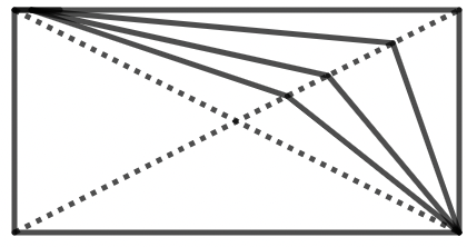
For the merged rectangle $I$, we use a series of straight line partitions to divide the rectangle into two equal-volume parts, which will be converted to a one-parameter model if we set the angle between the dividing line and horizontal line across the center $\theta$, where we suppose $0\leq\theta\leq\frac{\pi}{2}$. From simple calculations, we can conclude the arbitrary straight line must pass through the center of the rectangle. For convenience of notation, we set this partition model $\Omega_{\sim}=(\Omega_{1,\sim},\Omega_{2,\sim},Q_{3},\ldots,Q_{N})$ in two dimensional case.

For the rectangle

where $a_{1},a_{2},b$ are three positive constants. A straight line partition is used to divide the rectangle into two parts if we set the straight line parallel to the diagonal of $I$, and the distance from the intersection point $q$ to the endpoint at the upper right corner of $I$ is $b\in(0,\frac{2}{m})$.

For convenience of notation, we set this partition model

where $\Omega_{2,b,\sim}=I\setminus\Omega_{1,b,\sim}$.

Now, consider $d-$dimensional cuboid

and its two partitions $\Omega^{\prime}_{\sim}=(\Omega^{\prime}_{1,\sim},\Omega^{\prime}_{2,\sim})$ and $\Omega^{\prime}_{b,\sim}=(\Omega^{\prime}_{1,b,\sim},\Omega^{\prime}_{2,b,\sim})$ into two closed, convex bodies with

and

We choose $a_{1}=\frac{m-2}{m},a_{2}=\frac{m-1}{m},b=\frac{1}{m}$ in $\Omega^{\prime}_{1,\sim}$ and $\Omega^{\prime}_{1,b,\sim}$, denoted by $\Omega^{*}_{1,\sim}$ and $\Omega^{*}_{1,b,\sim}$, then we obtain

and

In this section, explicit $L_{2}-$discrepancy formulas are given for Class of partition model I and II.

The model [8] gives a family of unequivolume partitions in two dimensions with sampling number $N=2$, a certain type of symmetry along the $y=x$ diagonal is needed, and the partition is non-convex, expected $L_{2}-$discrepancy for $N=2,d=2$ attains optimal in these restrictions. It is also proved in [6] some class of convex partitions could minimize the expected $L_{2}-$discrepancy for $d-$dimensions with $N=m^{d}$, thus an interesting question is could some class of convex unequivolume partitions achieve better expected $L_{2}-$discrepancy formulas than the family of non-convex partitions for $d$ with $N=m^{d}$? The family of partitions in [8] is:

where $\Omega=\{(x,y)\in[0,1]^{2}:y\leq g(x)\}$. If $g(x)$ satisfies a highly nonlinear integral equation, then the partition is optimal. This result can be extended to $d-$dimensions with $N=m^{d}$ as the partition model 2.4 in [5], but it may be difficult to obtain an explicit expected $L_{2}-$discrepancy formula due to the difficulty in computing the solution of the integral equation that $g(x)$ has to satisfy. If we consider the convex partition, $g(x)$ will satisfy a linear equation, then an explicit formula is within reach. The optimal expected $L_{2}$-discrepancy formula may be obtained from the class of unequivolume partitions formed by a special class of linear equations, but we have not yet carried out the accurate calculation and comparison. Besides, since theorem 3.5 satisfies certain symmetry, it can be converted into a one-parameter model. Considering the partition class formed by general linear equations, the result should be a two-parameter model. As the equation satisfied by $g(x)$ becomes more and more complex, it is expected that the parameters contained in the $L_{2}-$discrepancy formula will become more complex, but it still has the value of numerical research, approximation error in (1.1) can still be accurately analyzed.

For some missing convex or non-convex partitions, we can naturally provide the following two examples, see Figure 7, similar to model 2.4, they can be easily extended to $d-$dimensions with $N=m^{d}$. Expected $L_{2}-$discrepancy formulas are also easy to compute if we follow the proof process of Theorem 3.1 and 3.5, because their partition curve equations can always be explicitly displayed by some parameters.

For equivolume partition $\mathbf{\Omega_{0,\sim}}=(\Omega_{1,\sim},\Omega_{2,\sim})$ of $I$(the same argument if we replace $\mathbf{\Omega_{0,\sim}}$ with $\mathbf{\Omega_{0,|}}$), from [Proposition $2$] in [5], which is, for an equivolume partition $\hat{\Omega}=\{\hat{\Omega}_{1},\hat{\Omega}_{2},\ldots,\hat{\Omega}_{N}\}$ of a compact convex set $K\subset\mathbb{R}^{d}$ with $\lambda(K)>0$, $P_{\hat{\Omega}}$ is the corresponding stratified sampling set, then

where

Through simple derivation, it follows that

and

Conclusion (4.3) is equivalent to the following

We first consider parameter $arctan\frac{1}{2}\leq\theta\leq\frac{\pi}{2}$, then we define the following two functions for simplicity of the expression.

and

where $\mathbf{x}=(x_{1},x_{2})$.

Furthermore, for $\mathbf{\Omega_{0,|}}=(\Omega_{1,|},\Omega_{2,|})$, (4.4) implies

and

Besides,

and

where $\Omega_{1,\sim}$, $\Omega_{2,\sim}$ denote subsets of partition $\mathbf{\Omega_{0,\sim}}$. In the following, we shall continue to divide subsets $\Omega_{1,\sim}=\{\Omega_{1,\sim,1},\Omega_{1,\sim,2}\}$ and $\Omega_{2,\sim}=\{\Omega_{2,\sim,1},\Omega_{2,\sim,2}\}$ to facilitate calculation. See Figures 8 to 9.

Therefore, for $\theta=\frac{\pi}{2}$, we introduce two symbols $B_{1,|},B_{2,|}$ and have

and

Thus,

Furthermore, we introduce $B_{1,\sim}$ and $B_{2,\sim}$, then

and

We divide our calculation into three steps. First, we compute $\int_{\Omega_{1,\sim}}x_{1}^{2}x_{2}^{2}d\mathbf{x}$, see Figure 8 for illustration.

Therefore, (4.9) and (4.10) imply

Second, we compute $\int_{\Omega_{2,\sim,1}}(x_{1}x_{2}-F(\mathbf{x}))^{2}d\mathbf{x}$ and $\int_{\Omega_{2,\sim,2}}(x_{1}x_{2}-G(\mathbf{x}))^{2}d\mathbf{x}$.

Thus, (4.12) and (4.13) imply

Combining (4.8), (4.11) and (4.14), we have

Third, we will compute $\int_{\Omega_{2,\sim,1}}F^{2}(\mathbf{x})d\mathbf{x}$ and $\int_{\Omega_{2,\sim,2}}G^{2}(\mathbf{x})d\mathbf{x}$ in the following.

In fact,

Combining (4.16) and (4.17), we have

Thus,

Therefore,

where $arctan\frac{1}{2}\leq\theta<\frac{\pi}{2}$.

For $\theta=\frac{\pi}{2}$, by (4.7) we have

Considering the case $0\leq\theta<arctan\frac{1}{2}$, we denote the partition by $\Omega^{\prime}_{\sim}=\{\Omega^{\prime}_{1,\sim},\Omega^{\prime}_{2,\sim}\}$, see Figure 10. Let

and

where

and

Then we divide subsets $\Omega^{\prime}_{1,\sim}=\{\Omega^{\prime}_{1,\sim,1},\Omega^{\prime}_{1,\sim,2}\}$ and $\Omega^{\prime}_{2,\sim}=\{\Omega^{\prime}_{2,\sim,1},\Omega^{\prime}_{2,\sim,2}\}$ to facilitate calculation. See Figure 10.

So

and

References

[1]J. Dick and F. Pillichshammer, On the mean square weighted discrepancy of randomized digital -nets over , Acta Arith., 117(2005), 371-403.
[2]L. L. Cristea, J. Dick and F. Pillichshammer, On the mean square weighted discrepancy of randomized digital nets in prime base, J. Complexity, 22(2006), 605-629.
[3]J. Dick and F. Pillichshammer, Discrepancy theory and quasi-Monte Carlo integration. In: W. W. L. Chen, A. Srivastav, G. Travaglini(eds.), Panoramy in Discrepancy Theory, Springer Verlag, Cham, 2014, 539-619.
[4]J. Dick, A. Hinrichs and F. Pillichshammer, A note on the periodic -discrepancy of Korobov’s -sets, Arch. Math. (Basel), 115(2020), 67-78.
[5]M. Kiderlen and F. Pausinger, On a partition with a lower expected -discrepancy than classical jittered sampling, J. Complexity, 70(2022), https://doi.org/10.1016/j.jco.2021.101616.
[6]M. Kiderlen and F. Pausinger, Discrepancy of stratified samples from partitions of the unit cube, Monatsh. Math., 195(2021), 267-306.
[7]N. Kirk and F. Pausinger, On the expected -discrepancy of jittered sampling, arXiv preprint arXiv:2208.08924, 2022.
[8]F. Pausinger, M. Rachh, S. Steinerberger, Optimal jittered sampling for two points in the unit square, Statist.Probab. Lett., 132(2018), 55–61.