Improved bounds in Weaver’s conjecture for high rank positive semidefinite matrices
Abstract.
Recently Marcus, Spielman and Srivastava proved Weaver’s conjecture, which gives a positive solution to the Kadison-Singer problem. In [Coh16, Br18], Cohen and Brändén independently extended this result to obtain the arbitrary-rank version of Weaver’s conjecture. In this paper, we present a new bound in Weaver’s conjecture for the arbitrary-rank case. To do that, we introduce the definition of -characteristic polynomials and employ it to improve the previous estimate on the largest root of the mixed characteristic polynomials. For the rank-one case, our bound agrees with the Bownik-Casazza-Marcus-Speegle’s bound when [BCMS19] and with the Ravichandran-Leake’s bound when [RL20]. For the higher-rank case, we sharpen the previous bounds from Cohen and from Brändén.
1. Introduction
1.1. The Kadison-Singer problem
The Kadison-Singer problem, posed by Richard Kadison and Isadore Singer in 1959 [KS59], is a fundamental problem that relates to a dozen areas of research in pure mathematics, applied mathematics and engineering. Basically, it asked whether each pure state on the diagonal subalgebra to has a unique extension. This problem was known to be equivalent to a large number of problems in analysis such as the Anderson Paving Conjecture [And79, And79, And81], Bourgain-Tzafriri Restricted Invertibility Conjecture [BT89, CT06], Feichtinger Conjecture [BS06, CCLV05, Gr03] and Weaver Conjecture [Wea04].
In a seminal work [MSS15b], Marcus, Spielman and Srivastava resolved the Kadison-Singer problem by proving the Weaver’s conjecture. The case of Weaver’s conjecture can be stated as follows.
Conjecture 1.1.
() There exist universal constants and such that the following holds. Let satisfy for all and
| (1.1) |
for every unit vector . Then there exists a partition of such that
| (1.2) |
for every unit vector and each .
The following theorem plays an important role in their proof of Weaver’s conjecture.
Theorem 1.2.
( see [MSS15b, Theorem 1.4] ) Let and let be independent random positive semidefinite Hermitian matrices in of rank 1 with finite support. If
and
then
| (1.3) |
Theorem 1.3 directly follows from Theorem 1.2 and implies a positive solution to Weaver’s conjecture.
Theorem 1.3.
( see [MSS15b, Corollary 1.5] ) Let be an integer. Assume that are positive semidefinite Hermitian matrices of rank at most such that
Let . Then there exists a partition such that
| (1.4) |
1.2. Related work
Here we briefly introduce the previous improvements on Theorem 1.3.
1.2.1. The rank-one case
When , Bownik, Casazza, Marcus and Speegle [BCMS19] improves the upper bound in (1.4) to when . This bound implies the same result in Conjecture 1.1, but with any constant . To our knowledge, this is the best known estimate on the constant in Conjecture 1.1.
Ravichandran and Leake in [RL20] adapted the method of interlacing families to directly prove Anderson’s paving conjecture, which is well-known to be equivalent to Weaver’s conjecture. They showed that, for any integer and any real number , if is a positive semidefinite matrix satisfying and for all , then there exists a partition such that
| (1.5) |
Here, denotes the submatrix of with rows and columns indexed by . Their result implies that the upper bound in (1.4) can be improved to
| (1.6) |
when . To see this, we write for each and set where . Then (1.6) immediately follows since
for each . When , Ravichandran and Leake’s bound in (1.6) coincides with the estimate of Bownik et. al. from [BCMS19]. In [AB20], Alishahi and Barzegar extended Ravichandran and Leake’s result to the case of real stable polynomials and studied the paving property for strongly Rayleigh process.
1.2.2. The higher-rank case
In [Coh16], Cohen showed that Theorem 1.3 holds for matrices with higher ranks and the upper bound in (1.4) still holds in this case. Brändén also got rid of the rank constraints in [Br18] and extended Theorem 1.3 to the realm of hyperbolic polynomials. For each and each integer , let be defined as
| (1.7) |
In the setting of Theorem 1.3, Brändén proved that, if the rank of each is at most , then the upper bound (1.4) can be improved to when . For the case where and , Brändén also obtained the same bound with that of [BCMS19]. One can check that Ravichandran and Leake’s bound (1.6) is better than ’s bound when and , but ’s bound is more general since it is available for .
1.3. Our contribution
In this paper we focus on extending the results in Theorem 1.2 and Theorem 1.3 to the higher-rank case. We first present the following theorem, which improves the previous bounds from (1.3) and from[Br18, Theorem 6.1].
Theorem 1.4.
Let be an integer and let . Let be independent random positive semidefinite Hermitian matrices in with finite support. Suppose that and
Then,
We immediately obtain the following corollary with a similar argument in [MSS15b, Corollary 1.5].
Corollary 1.5.
Let and be integers. Assume that are positive semidefinite Hermitian matrices of rank at most such that
| (1.8) |
Let . If , then there exists a partition such that
| (1.9) |
Proof.
Remark 1.6.
Motivated by the argument in [FY19, Proposition 2.2], we can relax the condition (1.8) in Corollary 1.5 to . More specifically, we can find rank-one matrices with trace at most such that . Then there exists an partition of satisfying (1.9) by Corollary 1.5. We can get a desired partition of by restricting each subset in the partition of to .
Our bound in (1.9) coincides with that of [RL20] for each when . In particular, our bound is also the same with that of [BCMS19] when and . For the case when , our bound (1.9) slightly improves Brändén’s bound, i.e., . We summarize the related works in Table 1.3.
| The value of and | Paving bound in (1.9) |
|---|---|
| for [BCMS19, RL20, Br18] | |
| [MSS15b] | |
| for [RL20] | |
| [Coh16] | |
| for [Br18] | |
| for [Br18] | |
| for (Corollary 1.5) |
We next provide an application of Corollary 1.5, which specifies a simultaneous paving bound for multiple positive semidefinite Hermitian matrices. In [RS19], Ravichandran and Srivastava proved a simultaneous paving bound for a tuple of zero-diagonal Hermitian matrices. Therefore, the following corollary serves as a counterpart of [RS19, Theorem 1.1]. The result also coincides with [RL20, Theorem 2] when paving just one matrix.
Corollary 1.7.
Let and be integers. Assume that are positive semidefinite Hermitian matrices satisfying for . Let . If , then there exists a partition such that
1.4. Our techniques
To introduce our techniques, let us briefly recall the proof of Theorem 1.2 and how [Coh16] and [Br18] extended Theorem 1.2 to the higher-rank case.
For the rank-one case, let be as defined in Theorem 1.2. For , let the support of be . In [MSS15b], Marcus, Spielman and Srivastava showed that the characteristic polynomials of form a so-called interlacing family. This implies that there exists a polynomial in this family whose largest root is at most that of the expectation of the characteristic polynomial of . Hence, it is enough to estimate the largest root of this expected characteristic polynomial. This expected characteristic polynomial is referred to as the mixed characteristic polynomial:
Definition 1.8.
(see [MSS15b]) Given , the mixed characteristic polynomial of is defined as
| (1.13) |
Assume that are independent random matrices of rank one in satisfying for each . Marcus, Spielman and Srivastava in [MSS15b, Theorem 4.1] showed that
| (1.14) |
Based on the above formula, they employed an argument of the barrier function that was developed in [BSS12] to estimate the largest root of the mixed characteristic polynomials.
For the higher-rank case, instead of studying the characteristic polynomials of , the authors of [Coh16] and [Br18] concentrated their attention on the mixed characteristic polynomials of . They showed that this family of polynomials also form an interlacing family. Furthermore, they proved that, for any positive semidefinite Hermitian matrices , the operator norm of is upper bounded by the largest root of , i.e.
Hence, the original problem is reduced to estimating the largest root of the expectation of the mixed characteristic polynomials, which can be done with a similar argument of barrier function.
To prove Theorem 1.4, we follow the above framework of [Coh16] and [Br18]. Our main technique is that we derive a new formula for the mixed characteristic polynomials (see Theorem 3.8). Based on this new formula and the method of barrier function, we obtain an improved estimate on the largest root of the mixed characteristic polynomials. We state it as follows.
Theorem 1.9.
Assume that are positive semidefinite Hermitian matrices of rank at most such that . Let . If , then we have
| (1.15) |
1.5. Organization
This paper is organized as follows. After introducing some useful notation and lemmas in Section 2, we introduce the definition of -characteristic polynomials, showing the connection between -characteristic polynomials and the mixed characteristic polynomials in Section 3. In Section 4, we use the method of barrier function to present a proof of Theorem 1.9. The proof of Theorem 1.4 is presented in Section 5.
2. Preliminaries
2.1. Notations
We first introduce some notations. For a vector , we let denote its Euclidean 2-norm. For a matrix , we use to denote its operator norm. We write to indicate the partial differential . For each , let denote the vector whose -th entry equals and the rest entries equal to . For a polynomial with real roots, we use and to denote the maximum and minimum root of respectively.
For an integer , we use to denote the set . For any two positive integers and , we call an -partition of if are disjoint and . We use the notation to denote the set of all -partitions of .
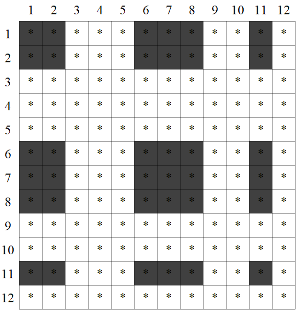
Given a matrix , for a subset , we use to denote the principal submatrix of whose rows and columns are indexed by . Let be an integer. Given a matrix , for , we use to denote the principal submatrix . For example, let and let . If we set , then for a matrix the principal submatrix is composed of the shaded part in Figure 1.
2.2. Interlacing families
The method of interlacing families is a powerful tool to show the existence of some combinatorial objects. Marcus, Spielman and Srivastava employed this tool to prove the existence of bipartite Ramanujan graphs of all sizes and degrees, solved the Kadison-Singer problem and proved a sharper restricted invertibility [MSS15a, MSS15b, MSS17, MSS18].
Here we recall the definition and related results of interlacing families from [MSS15b]. Throughout this paper, we say that a univariate polynomial is real-rooted if all of its coefficients and roots are real.
Definition 2.1.
(see [MSS15b, Definition 3.1] ) We say a real-rooted polynomial interlaces a real-rooted polynomial if . For polynomials , if there exists a polynomial that interlaces for each , then we say that have a common interlacing.
We next introduce the definition of interlacing families.
Definition 2.2.
(see [MSS15b, Definition 3.3] ) Assume that are finite sets. For every assignment , let be a real-rooted degree polynomial with positive leading coefficient. For each and each partial assignment , we define
We also define
We say that the polynomials form an interlacing family if for all integers and all partial assignments , the polynomials have a common interlacing.
We state the main property of interlacing families as the following lemma.
Lemma 2.3.
(see [MSS15b, Theorem 3.4] ) Assume that be finite sets and let be an interlacing family. Then there exists some such that the largest root of is upper bounded by the largest root of .
2.3. Real stable polynomials
Through our analysis, we exploit the notion of real stable polynomials, which can be viewed as a multivariate generalization of real-rooted polynomials. For more details, see [BB10, Wag11].
We first introduce the definition of real stable polynomials.
Definition 2.4.
A polynomial is real stable if for all with and .
To show the polynomial we concern in this paper is real stable, we need the following lemma.
Lemma 2.5.
(see [BB08, Proposition 2.4] ) For any positive semidefinite Hermitian matrices and any Hermitian matrix , the polynomial
| (2.1) |
is either real stable or identically zero.
Real stability can be preserved under some certain transformations. In our proof, we use some real stability preservers to reduce multivariate polynomials to a univariate one which is a real-rooted polynomial.
Lemma 2.6.
(see [Wag11, Lemma 2.4] ) If is real stable and , then the following polynomials are also real stable:
-
•
,
-
•
, for all ,
-
•
, for all .
2.4. The mixed characteristic polynomial
The mixed characteristic polynomial plays a key role in the proof of Theorem 1.2. In this subsection we introduce some basic properties of mixed characteristic polynomials which is useful in our proof of Theorem 1.4.
Lemma 2.7.
Lemma 2.8.
It is also pointed out by Brändén in [Br18] that the mixed characteristic polynomial is affine linear in each , i.e., for all and all :
| (2.4) | ||||
where . Hence, if are independent random matrices with finite support, then we have
| (2.5) |
3. A new formula for mixed characteristic polynomials
For positive integers and , we first introduce the -determinant and -characteristic polynomial of a matrix . Then we show some connections between -characteristic polynomials and mixed characteristic polynomials. Recall that we use to denote the set of all -partitions of . Also recall that for each and each we use to denote the principal submatrix of with rows and columns indexed by .
Definition 3.1.
Let be two positive integers. For any matrix , the -determinant of is defined as
The -characteristic polynomial of is defined as
| (3.1) |
Remark 3.2.
A simple calculation shows that is a monic polynomial of degree . For , we have , and is the regular characteristic polynomial of . If we take , then is a multiple of the -th order derivative of the characteristic polynomial of (see Proposition 3.3).
We next introduce some connections among and other generalizations of the determinant and the characteristic polynomial in the literature.
-
1.
(Borcea-Brändén [BB08]) For a -tuple of matrices in , the mixed determinant, first introduced by Borcea and Brändén in [BB08], is defined as
Note that is the regular characteristic polynomial of . In [BB08], Borcea and Brändén used the notion of the mixed determinant to prove a stronger version of Johnson’s Conjecture. We remark here that the -determinant introduced in Definition 3.1 can be viewed as a generalization of the mixed determinant by the following identity:
(3.2) where is a block diagonal matrix.
-
2.
(Ravichandran-Leake [RL20]) For a matrix , the -characteristic polynomial of the matrix is defined as (see [RL20, Proposition 2])
(3.3) Ravichandran and Leake used the -characteristic polynomial to prove Anderson’s paving formulation of Kadison-Singer problem [RL20]. It is easy to see the relationship between and :
(3.4) -
3.
(Ravichandran-Srivastava [RS19]) For a -tuple of matrices in , the mixed determinantal polynomial is defined as
(3.5) Ravichandran and Srivastava used the mixed determinantal polynomial to provide a simultaneous paving of a -tuple of zero-diagonal Hermitian matrices [RL20]. According to (3.2), we immediately have the following identity:
(3.6) Hence, the -characteristic polynomial can be considered as a generalization of the mixed determinantal polynomial.
We next provide several basic properties about the -characteristic polynomial. The first one provides an alternative expression of -characteristic polynomial.
Proposition 3.3.
Let be two positive integers. Let
Then, for any matrix , we have
| (3.7) |
Remark 3.4.
Proposition 3.3 can be considered as a generalization of [RL20, Proposition 1] and [RS19, Proposition 2.3], which express the -characteristic polynomial and the mixed determinantal polynomial both in differential formulas. In [RL20], Ravichandran and Leake showed that
for matrix , where . In [RS19], Ravichandran and Srivastava showed that
for matrices . These two formulas correspond to the case where is a block-diagoal matrices in Proposition 3.3.
Proof of Proposition 3.3.
To prove the conclusion, according to (3.1), it is enough to show that
A simple calculation shows that the following algebraic identity holds for any polynomial :
| (3.8) |
For with , we have
which implies
| (3.9) |
where is a polynomial which has degree in each . Now we define the polynomial
| (3.10) |
for each . We set
where
For each , we use (3.9) to obtain that
| (3.11) |
A simple calculation shows that
| (3.12) |
Also note that, for each , we have
| (3.13) |
where is defined as
| (3.14) |
Combining (3.11), (3.12) and (3.13), we obtain that, for each ,
| (3.15) | ||||
In particular, when , we have
| (3.16) |
Combining (3.10) and (3.16), we obtain that
∎
The next proposition shows that is real-rooted if is Hermitian.
Proposition 3.5.
Let be two positive integers. For any Hermitian matrix , the -characteristic polynomial is real-rooted.
Proof.
Since is Hermitian, by Lemma 2.5, we see that the polynomial
is either real stable or identically zero. If it is zero, then we are done. We assume that . Lemma 2.6 shows that the differential operator and setting all variables to preserve real stability. Then, by Proposition 3.3, we conclude that is a univariate real stable polynomial, which is real-rooted. ∎
We next present several properties about the roots of the -characteristic polynomial of a Hermitian matrix .
Proposition 3.6.
Let be two positive integers. Assume that is a Hermitian matrix. Then we have the following results:
-
(i)
The sum of the roots of equals .
-
(ii)
For any vector we have
(3.17) -
(iii)
If is positive semidefinite, then we have
(3.18)
Proof.
(i) We use to denote the sum of the roots of . Since is a real-rooted polynomial of degree with leading coefficient being , it is known that equals the negative value of the coefficient of in . Note that, for each -partition of , the characteristic polynomial of is of the form
According to (3.1), we have
| (3.19) |
Observing that each diagonal entry of appears in exactly distinct -partitions of , we can rewrite equation (3.19) as
which gives the desired result.
(ii) For each we set
According to Proposition 3.5, is real-rooted for each . Define as
Since the maximal root of a real-rooted polynomial is continuous in its coefficients, we obtain that is a continuous function. Also note that
| (3.20) |
Hence, it is enough to show that is monotone increasing in which implies and hence (3.17).
According to Definition 3.1 we have
where denotes the subvector of by extracting the entries of indexed by . Note that, for each , is a polynomial in of degree at most one, which implies that we can write in the form of
| (3.21) |
We next prove that is monotone by contradiction. For the aim of contradiction, we assume that is not monotone. Since is continuous, there exist such that and . We use (3.21) to obtain
which implies
| (3.22) |
Then we substitute (3.22) into (3.21) and obtain for any . By the definition of , this means that for any . Let . Since is not monotone, we have . Set . By continuity, there exist such that and . Then the preceding argument shows that for any , which contradicts with . Hence, is monotone.
We next show that is monotone increasing. Let denote the sum of the roots of . It follows from (i) that
Hence, when , we have . Since , we have
with . Thus, is monotone increasing in which implies . We arrive at the conclusion.
(iii) By the spectral decomposition, we can write
where is the unit-norm eigenvector of corresponding to the -th largest eigenvalue . Since is positive semidefinite, we have for each . According to (3.17), we have
| (3.23) |
A simple calculation shows that
which implies
| (3.24) |
Since is positive semidefinite, its operator norm is exactly . Hence, combining (3.23) with (3.24), we arrive at
∎
Remark 3.7.
Inspired by [RS19, Lemma 5.5], we next show a connection between the -characteristic polynomial and the mixed characteristic polynomial, which is the main result of this section.
Theorem 3.8.
Let be matrices of rank at most . Suppose that and satisfy
We set for all and
| (3.26) |
Then, we have
Proof.
For each , let be the random rank one matrix taking values in
with equal probability. Then, we have
For each subset and each , we let denote the submatrix of and , respectively, obtained by extracting the columns indexed by . Now a simple calculation shows
Note that for each we have
Hence, we arrive at
∎
Remark 3.9.
Note that where is presented in (3.26). We next assume that are positive semidefinite. Combining Proposition 3.5 and Theorem 3.8, we obtain that is real-rooted, which conincides with the well-known result in [MSS15b, Corollary 4.4]. Note that
It immediately follows from Theorem 3.8 that
| (3.27) |
Also note that
| (3.28) |
Combining Proposition 3.6 (iii) , (3.27) and (3.28), we obtain that
| (3.29) |
which is the same with the result in Proposition 2.7.
4. Proof of Theorem 1.9
The aim of this section is to prove Theorem 1.9, which shows an upper bound for the maximum root of . To do that, we first present an upper bound of the maximum root of , and then we employ the connection between and (see equation (3.27)) to prove Theorem 1.9.
Theorem 4.1.
Let and be two positive integers. Assume that is a positive semidefinite Hermitian matrix such that . Set
If , then we have
| (4.1) |
Remark 4.2.
We next give a proof of Theorem 1.9. The proof of Theorem 4.1 is postponed to the end of this section.
Proof of Theorem 1.9.
Recall that are positive semidefinite Hermitian matrices of rank at most such that . Suppose that are the vectors in such that
We set and set . Note that
Since and have the same nonzero eigenvalues, we obtain
Moreover, for each we have
Since , Theorem 4.1 gives
which implies
Here, we use Theorem 3.8, i.e.,
∎
In the remainder of this section, we aim to prove Theorem 4.1 by adapting the method of multivariate barrier function. We first introduce the barrier function of a real stable polynomial (see also [MSS15b]).
Definition 4.3.
Let be a multivariate polynomial. We say that a point is above the roots of if for all . We use to denote the set of points that are above the roots of .
Definition 4.4.
Let be a real stable polynomial. The barrier function of at a point in the direction is defined as
| (4.3) |
Here we briefly introduce our proof of Theorem 4.1. According to Proposition 3.3, we have
where . For Hermitian matrix , we consider the real stable polynomial
| (4.4) |
where
| (4.5) |
We iteratively define the polynomials
| (4.6) |
We start with an initial point with that is above the roots of . For each , we aim to find a positive number such that each entries of less than or equal to , which implies the result in Theorem 4.1.
We need the following result which depicts the behavior of barrier functions of polynomials affected by taking derivatives.
Proposition 4.5.
[RL20, Proposition 9, Proposition 10] Let be any integer. Assume that is a real stable polynomial of degree in . Let and let be the smallest root of the univariate polynomial . Let
| (4.7) |
Then, we have and
We introduce a well-known result of the zeros of the real stable polynomials (see also [RL20, Proposition 8]).
Lemma 4.6.
[Tao13, Lemma 17] Let be a real stable polynomial of degree in . For each , denote the roots of the univariate polynomial by . Then for each , the map defined on is non-increasing.
The following lemma is useful for our analysis.
Lemma 4.7.
Let be a positive semidefinite Hermitian matrix. Set
| (4.8) |
Assume that . Then, for each , the smallest root of the univariate polynomial is non-negative.
Proof.
We can write in the form of , where are both positive semidefinite Hermitian and . Since , we obtain that is positive definite. Set . Noting that is a principal submatrix of , we obtain that is positive definite. We use the Schur complement to obtain that
Hence, the roots of are the eigenvalues of the positive semidefinite matrix , which implies that all roots of are non-negative. ∎
Proposition 4.8.
Proof.
By equation (3.15), we can write the univariate polynomial in the form of
where
and is defined in (3.14). Since , we have
which implies that the principal matrix
Then we obtain that . Lemma 4.7 shows that the smallest root of the polynomial
is non-negative. Since is a multiple of the sum of monic polynomials whose smallest root is non-negative, it follows that the smallest root of is non-negative. ∎
We need the following lemma to provide an estimate on the value of .
Lemma 4.9.
Let be two positive integers. Let be a positive semidefinite Hermitian matrix satisfying . Set
Let be defined as in (4.4). Then for any we have
Proof.
Define the polynomial
where
By equation (3.8), for each , we have
| (4.9) |
For each , we have
where denotes the principle submatrix of whose the -th row and -th column are deleted. By the expression of the inverse of a matrix, we obtain that
| (4.10) |
Taking the -th diagonal element of each side of (4.10), we have
Then for each , we have
| (4.11) |
Combining (4.9) and (4.11), we obtain that
Suppose that the spectral decomposition of is
| (4.12) |
where is a unitary matrix and is a diagonal matrix of eigenvalues of . It follows that . Thus we have
| (4.13) | ||||
Set for each . Then we have
| (4.14) | ||||
Here, we use the following inequality:
where and . Note that
| (4.15) |
since each column of is a unit vector. We use (4.12) to obtain that
Then we have
| (4.16) | ||||
Thus, combining (4.14), (4.15) and (4.16), we obtain that
∎
Now we have all the materials to prove Theorem 4.1.
Proof of Theorem 4.1.
Suppose that is a constant which is chosen later. Set . Let be defined as in (4.4). According to , we obtain that is above the roots of . Recall that
A simple observation is that
Hence, to prove the conclusion, it is enough to show that is above the roots of . For each , set
where
Let be the smallest root of the univariate polynomial
| (4.17) |
By Proposition 4.5 , we have and
| (4.18) |
we claim that
| (4.19) |
Noting that is above the roots of , we can use (4.19) to obtain the conclusion.
It remains to prove (4.19). We first show that for each . For each we define the univariate polynomial
| (4.20) |
Since and , we obtain that
| (4.21) |
where the first inequality follows from Lemma 4.6 and the second inequality follows from Proposition 4.8. Then, combining (4.21), (4.18) and Lemma 4.9, for each , we have
So, for each , we have
| (4.22) |
Set . A simple calculation shows that
where the equality holds if and only if , i.e.,
This implies that if , i.e., , then
| (4.23) |
5. Proof of Theorem 1.4
Proof of Theorem 1.4.
For each , let be the support of . By Lemma 2.8, we see that the polynomials
form an interlacing family. Then Lemma 2.3 implies that there exists such that
| (5.1) |
Combining (2.5) and (5.1), we obtain that
| (5.2) |
Since
and , Theorem 1.9 gives
Finally, combining Lemma 2.7 and (5.2) we arrive at
This implies the desired conclusion.
∎
References
- [AB20] K. Alishahi and M. Barzegar, Paving property for real stable polynomials and strongly rayleigh processes, arXiv preprint arXiv:2006.13923, 2020.
- [And79] J. Anderson, Extensions, restrictions, and representations of states on -algebras, Trans. Amer. Math. Soc., 249 (1979), 303-329. MR 0525675. Zbl 0408. 46049. http://dx.doi.org/10.2307/1998793.
- [And79] J. Anderson, Extreme points in sets of positive linear maps on , J. Funct. Anal., 31 (1979), 195-217. MR 0525951. Zbl 0422.46049. http://dx.doi.org/10. 1016/0022-1236(79)90061-2.
- [And81] J. Anderson, A conjecture concerning the pure states of and a related theorem, in Topics in Modern Operator Theory (Timisoara/Herculane, 1980), Operator Theory: Adv. Appl. 2, Birkhuser, Boston, 1981, pp. 27-43. MR 0672813. Zbl 0455.47026.
- [BSS12] J. Batson, D. A. Spielman, and N. Srivastava, Twice-Ramanujan sparsifiers, SIAM J. Comput. 41 (2012), 1704-1721. MR 3029269. Zbl 1260.05092. http: //dx.doi.org/10.1137/090772873.
- [BB08] J. Borcea and P. Brändén Applications of stable polynomials to mixed determinants: Johnson’s conjectures, unimodality, and symmetrized Fischer products, Duke Math. J. 143 (2008), 205-223. MR 2420507. Zbl 1151.15013. http://dx.doi.org/10.1215/00127094-2008-018.
- [BB10] J. Borcea and P. Brändén, Multivariate Pólya-Schur classification problems in the Weyl algebra, Proceedings of the London Mathematical Society, 101(1):73-104, 2010.
- [BT89] J. Bourgain and L. Tzafriri, Restricted invertibility of matrices and applications, in Analysis at Urbana, Vol. II (Urbana, IL, 1986-1987), London Math. Soc. Lecture Note Ser. 138, Cambridge Univ. Press, Cambridge, (1989), pp. 61-107. MR 1009186. Zbl 0698.47018. http://dx.doi.org/10.1017/CBO9781107360204.006.
- [BCMS19] M. Bownik, P. Casazza, A. Marcus and D. Speelge Improved bounds in Weaver and Feichtinger conjectures, Journal für die reine und angewandte Mathematik (2019), 749:267-293
- [BS06] M. Bownik and D. Speegle, The Feichtinger conjecture for wavelet frames, Gabor frames and frames of translates, Canad. J. Math. 58 (2006), no. 6, 1121-1143.
- [Br11] P. Brändén Obstructions to determinantal representability. Advances in Mathematics, 226(2):1202-1212, 2011.
- [Br18] P. Brändén Hyperbolic polynomials and the Kadison-Singer problem, In arXiv preprint. https://arxiv.org/pdf/1809.03255, 2018.
- [CCLV05] P. Casazza, O. Christensen, A. Lindner and R. Vershynin, Frames and the Feichtinger conjecture, Proc. Amer. Math. Soc. 133 (2005), no. 4, 1025-1033.
- [CT06] P. G. Casazza and J. C. Tremain, The Kadison-Singer problem in mathematics and engineering, Proc. Natl. Acad. Sci. USA 103, (2006), 2032-2039. MR 2204073. Zbl 1160.46333. http://dx.doi.org/10.1073/pnas.0507888103.
- [Coh16] M. Cohen, Improved Spectral Sparsification and Kadison-Singer for Sums of Higher-rank Matrices, 2016, from http://www.birs.ca/events/2016/5-day-workshops/16w5111/videos/watch/201608011534-Cohen.html.
- [FY19] O. Friedland and P. Youssef. Approximating matrices and convex bodies, International Mathematics Research Notices, 2019(8):2519–2537, 2019.
- [Gr03] K. Grchenig, Localized frames are finite unions of Riesz sequences, Adv. Comput. Math. 18 (2003), no. 2-4, 149-157.
- [KS59] R. V. Kadison and I. M. Singer, Extensions of pure states, Amer. J. Math., 81 (1959), 383-400. MR 0123922. Zbl 0086.09704. http://dx.doi.org/10.2307/ 2372748.
- [LPR05] A. Lewis, P. Parrilo, and M. Ramana. The lax conjecture is true. Proceedings of the American Mathematical Society, 133(9): 2495-2499, 2005.
- [MSS15a] A. Marcus, D. A. Spielman, and N. Srivastava, Interlacing families I: Bipartite Ramanujan graphs of all degrees, Ann. of Math. 182 (2015), 307-325. http://dx.doi.org/10.4007/2015.182.1.7.
- [MSS15b] A. Marcus, D. A. Spielman, and N. Srivastava, Interlacing families II: mixed characteristic polynomials and the Kadison-Singer problem, Ann. of Math. (2) 182, no. 1 (2015): 327-350.
- [MSS17] A. W. Marcus, D. A. Spielman, and N. Srivastava, Interlacing Families III: Sharper restricted invertibility estimates, arXiv: 1712.07766, 2017, to appear in Israel J. Math.
- [MSS18] A. W. Marcus, D. A. Spielman, and N. Srivastava, Interlacing families IV: Bipartite ramanujan graphs of all sizes, SIAM Journal on Computing, 47(6): 2488-2509, 2018.
- [Rav20] M. Ravichandran, Principal submatrices, restricted invertibility and a quantitative Gauss-Lucas theorem, International Mathematics Research Notices, Volume 2020, Issue 15, August 2020, Pages 4809-4832, https://doi.org/10.1093/imrn/rny163.
- [RL20] M. Ravichandran and J. Leake, Mixed determinants and the Kadison-Singer problem., Mathematische Annalen (2020) 377:511-541 https://doi.org/10.1007/s00208-020-01986-7
- [RS19] M. Ravichandran and N. Srivastava, Asymptotically Optimal Multi-Paving, International Mathematics Research Notices, (2019) Vol. 00, No. 0, pp. 1-33 doi:10.1093/imrn/rnz111
- [Tao13] T.Tao, Real stable polynomials and the Kadison-Singer problem, 2013, from https://terrytao.wordpress.com/2013/11/04/real-stable-polynomials-and-the-kadison-singer-problem/#more-7109.
- [Wag11] D. Wagner, Multivariate stable polynomials: theory and applications. Bulletin of the American Mathematical Society, 48(1):53-84, January 2011.
- [Wea04] N. Weaver, The Kadison-Singer problem in discrepancy theory, Discrete Math. 278 (2004), 227-239. MR 2035401. Zbl 1040.46040. http://dx.doi.org/10.1016/ S0012-365X(03)00253-X.