Implications of neutrino species number and summed mass measurements in cosmological observations
Abstract
We confront measurable neutrino degrees of freedom and summed neutrino mass in the early universe to particle physics at the energy scale beyond the standard model (BSM), in particular including the issue of neutrino mass type distinction. The Majorana-type of massive neutrino is perfectly acceptable by Planck observations, while the Dirac-type neutrino may survive in a restricted class of models that suppresses extra right-handed contribution to at a nearly indistinguishable level from the Majorana case. There is a chance that supersymmetry energy scale may be identified in supersymmetric extension of left-right symmetric model if improved measurements discover a finite value. Combined analysis of this quantity with the summed neutrino mass helps to determine the neutrino mass ordering pattern, if measurement accuracy of order, meV, is achieved, as in CMB-S4.
I Introduction
Discovery of non-vanishing neutrino masses by oscillation experiments requires extension of the electroweak standard model based on massless left-handed neutrinos. In general, both left and right handed neutrino fields, ( for the three neutrino scheme) and are introduced in this extension. Difference of Dirac and Majorana types of neutrino is in whether projected two-component mass eigenstates have mass degeneracy (Dirac case), or have two distinct masses (Majorana case), large and small ones. The mass degeneracy of Dirac neutrinos implies the law of lepton number conservation, while the Majorana neutrino violates the lepton number conservation.
The Majorana case provides the interesting seesaw mechanism explaining why ordinary neutrinos appearing in weak processes are very light (typically much smaller than ) with the electron mass) compared to all other fermions, being suppressed in proportion to by heavy masses, ’s [1]. The lepton number violation has a further consequence of interesting lepto-genesis scenario which explains the baryon asymmetry of our universe [2]. In this scenario the final baryon and the lepton number asymmetries are comparable in their magnitudes, of order , and excludes a possibility of large chemical potential for leptons. Experimental determination of Majorana or Dirac neutrino is thus one of the most outstanding problems that faces particle physics.
The plausible three-neutrino scheme predicts the neutrino species number (for a small deviation, see the note [3]) at nucleo-synthesis for three species of Majorana neutrinos. On the other hand, if the independent component in the Dirac-type neutrino fully contributes to the extra of neutrino species, the Dirac theory would predict in contradiction to cosmological observations. What usually happens is that decouples earlier from the rest of thermal particles, and after a series of subsequent reheating events their number density decreases relative to still in thermal equilibrium. The extent of diluted number density is estimated by the adiabatic relation of entropy conservation, and it gives an extra contribution to , usually time and temperature dependent, after decoupling.
Planck observations of cosmic mircowave background (CMB) provided a stringent value at CL [4]. This result is perfectly consistent with the Majorana-type neutrino, but barely consistent with the Dirac-type neutrino. There have been some discussions of how to understand this and a less stringent result, , if the neutrino mass is of Dirac type since Planck publication [5], [6], [7], [8]. We shall recapitulate the Dirac-type neutrino case improving calculation of decoupling temperature. Precision measurements in cosmological observations of CMB-S4 [9] is expected to determine this number accurately.
Improved future measurements including null result are expected to probe species number present in physics beyond the standard model (BSM), if the neutrino mass of Dirac type. We find it of particular interest to target supersymmetric extension of left-right symmetric model. In this case it becomes possible to identify SUSY scale if a finite is found, or lower energy scale if it is not found.
Our further task in the present paper is a combined analysis of the neutrino species number and the summed neutrino mass measurement: irrespective of Majorana or Dirac neutrinos, the analysis is shown to have a great impact on the neutrino mass ordering problem, the normal hierarchy (NH) or the inverted hierarchy (IH). We shall be able to provide a new perspective of what forthcoming observations imply to BSM physics.
The present paper is organized as follows. In the next section we explain some basic facts about the neutrino species number , and what cosmological observations of this quantity imply. The adiabatic entropy conservation is emphasized and calculation of the relativistic degrees of freedom in thermal medium of temperature becomes important. The Majorana-type of massive neutrino is found compatible with cosmological observations, while the Dirac-type neutrino requires new analysis, as done in the literature. In Section III theoretical framework for discussion of Dirac-type massive neutrino is pointed out. Calculation of right-handed decoupling in this framework is worked out in detail, since results in the literature lack details of these calculations. We present detailed explanation of production, adding processes not considered in the literature. It is shown that four-Fermi type approximation of pair production rate is sufficient to determine the thermalization condition and the decoupling temperature. In Section IV we discuss how the derived decoupling temperature is related to diluted and the necessary dilution may be realized in unification schemes. We may relate SUSY energy scale to and shall be able to discuss how supersymmetric left-right symmetric schemes are constrained. In Section V another important quantity of summed neutrino masses in future cosmological observations may be combined to neutrino oscillation data, and resulting plot in plane can be used to determine another neutrino property, normal and inverted mass hierarchical ordering.
Throughout this paper we use the unit of .
II Preliminary
II.1 at nucleo-synthesis and at epochs after recombination
The effective massless degrees of freedom determines the cosmic energy density, hence controls the speed of cosmic expansion. This quantity at nucleo-synthesis ( seconds since the big-bang) is measurable by comparing measured light element abundances with theoretical calculation, while the same quantity at later epochs after recombination ( years after the bang) is measured by Planck and CMB-S4 observations. The quantity at these two epochs is sensitive function of 4He abundance . The allowed region in the plane from observations is usually presented by contour maps. The important fact is that correlations given by the derivative signs of are opposite at two epochs, positive at nucleo-synthesis and negative at recombination. This makes it possible to determine both of and at high precision.
The primordial 4He abundance is around 0.25. Reference [10] on nucleo-synthesis cites a conservative bound , but also mentions a more restrictive bound . The correlation with at nucleo-synthesis gives a straight line in the plane, as reviewed in [9], ranging in . The final status of Planck 2018 + BAO observations gives an impressive upper bound at 95% CL [4].
Not only neutrinos, but also other stable light relics left behind from the early thermal history give additional contribution, extra per a single relic. Examples are axion, dark photon and sterile neutrino. Contribution from a spin-less stable light relic is . This quantity can also be negative if light relics are unstable and decay during two epochs. We shall assume that there is no such relic, or even if there is, their cumulative contribution is restricted at most by (CMB-S4 target value), and concentrate on diluted Dirac which may behave in a similar way to a light relic.
II.2 Adiabatic dilution factor and
Assume that in the Dirac theory is thermally abundant at early cosmological epochs, and calculate the amount of dilution. After decoupling the universe goes through many annihilation events of thermal anti-particles, thereby reheating the universe. Electroweak interaction is far stronger than interactions in BSM, hence left-handed is reheated, but is not. This gives rise to difference of and effective temperatures. Note that even after ’s decouple and become non-thermal, one can assign their effective temperature. This is because the entropy conservation of (with the time-dependent cosmic scale factor) holds at nearly instantaneous reheating processes. The entropy density is proportional to the massless degrees of freedom in radiation-dominated epoch. Hence one can readily calculate the temperature ratio before and after rehearing events by counting respective species number contributing to .
Assuming that the standard electroweak phase transition took place in the Big Bang Universe, it is straightforward to evaluate in the era up to the electroweak phase transition in the standard model.
Fermions are counted by the weight for one spin state and bosons by the weight . Counting gives the dilution factor in terms of number density ratio, , since the electroweak phase transition.
We summarize factors relevant to dilution in the following table, Table(1) in which indicates the species number at cosmological events i.
| i | EW | S4 | ||
|---|---|---|---|---|
| 10.75 | 106.75 | 124.75 | 360 | |
| 3 | 0.14 | 0.11 | 0.028 |
It is convenient in the rest of analysis to relate the extra to the extra relativistic degrees of freedom ,
| (1) |
where is the species number of electroweak theory, and . Note that can be negative, implying that decoupling may occur below the electroweak temperature GeV.
Alternatively, one can relate upper bound or observed value to required value, using the formula (1).
III Fate of right-handed neutrino of Dirac type
III.1 Theory of Dirac-type massive neutrino
Let us first recall what happens in the standard electroweak theory based on the gauge group SU(2)U(1), when one introduces the right-handed neutrino . It is known that introduction of SU(2)U(1) singlet opens the possibility of Higgs boson () coupling proportional to doublet bi-linear fermion which, after the spontaneous electroweak gauge symmetry breaking, gives the Dirac-type neutrino mass. Inevitable process from thermal produces , but with a negligible amount of () if neutrino masses are less than of order 100 eV [10]. There seems nothing wrong with this scheme, but this minimum extension does not give any clue to many outstanding problems of particle physics such as generation of the baryon asymmetry. We need a new theoretical framework of massive Dirac-type neutrino.
A natural scheme is grand unified gauge theories (GUT), but it is sufficient to first think of an intermediate step of subgroup unification towards GUT. We find it most natural to analyze dilution in the left-right symmetric extension of the standard electroweak theory, SU(2)SU(2)U(1) gauge theory [11], as also made in [7]. The Higgs system consists of irreducible representations, of SU(2)SU(2)L group. Regarding all species of particle as massless, there are 18 extra in addition to the standard one and three right-handed neutrinos .
Some details of this doublet left-right symmetric model (DLRSM) are given in Appendix.
III.2 Decoupling of thermalized right-handed neutrinos in LR symmetric model
The Boltzmann equation for the number density, obtained after integrating the distribution function in the phase space (space volume times the momentum-space volume in spatially homogeneous universe), describes time evolution in the expanding universe. Consider a number density of species . The equations is
| (2) |
with the Hubble rate ( the energy density of effectively massless particles, ). When the Hubble rate compared with right-hand side (RHS) is small, thermal equilibrium is realized with vanishing RHS of (2) (meaning the positive production and the negative destruction balance). This thermal equilibrium is ended at decoupling temperature that is determined by equating the rate to the Hubble rate, . One may use for annihilation rate
| (3) | |||
| (4) |
Momenta of initial and final particles, assumed massless, are denoted , respectively. Lorentz-invariant squared amplitude summed over spin states is written in terms of invariant variables, . They are calculated below. is the number density of initial thermal ( is its spin).
One may separately confirm that thermalization condition is satisfied by considering inverse processes. Since we treat all initial and final fermions as massless (actually much lighter than gauge bosons ) inverse production process has equal rate to the annihilation rate. Thus, time integrated quantity gives thermally summed number density.

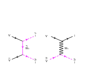
Relevant annihilation processes of right-handed neutrino (conjugate processes of production to be included as well) in LR symmetric models occur via two-body colliding processes of many kinds. Typical Feynman diagrams are depicted in Fig(1). In order to calculate rate, we classify individual contributions as
| (5) | |||
| (6) | |||
| (7) | |||
| (8) | |||
| (9) |
with being quarks and charged lepton. We note that process involving light higgs pair is absent, because a neutral scalar field has no vector current that may couple to . Feynman rules for amplitude and rate calculation can readily be extracted using formulas in Appendix.
A part of these contributions to annihilation rates have been calculated in the literature. Their substantial part is missing in the literature, and we shall cover and add all relevant contributions. The decoupling temperature at which two rates are equal is related to right-handed gauge coupling masses and gauge coupling . Remarkably, we shall be able to provide analytic results for important quantities we need.
SU(2)SU(2)U(1) gauge theory gives contributions from listed in (5) (9), some of them depicted in Fig(1). Invariant squared amplitudes after spin summation consist of coupling factors and dynamical parts given in terms of variables. Listed contributions have different dependence. It is sufficient to calculate in the temperature range gauge boson masses, hence four-Fermi approximation is excellent, with the common strength factor ,
| (10) |
We used notations for masses, to distinguish from ordinary electroweak gauge bosons , and are gauge coupling constant and mixing angle in the SU(2)R sector. Flavor dependent coupling factors are further multiplied to squared Fermi constant;
| (11) | |||
| (12) | |||
| (13) | |||
| (14) |
Contributions in squared amplitudes arise from type of diagrams in Fig(1) and those of type of exchanged gauge bosons. For instance, is from squared channel exchange of Fig(1a) in which leptons are replaced by relevant quarks .
The last coupling arises from interference contribution of t-channel -exchange (a) diagram and s-channel -exchange (b) diagram for two-body process of . As explained in Appendix, a value should be used. Using these couplings, squared invariant amplitudes are given by
| (15) |
The last integral over final states in (4) is to be calculated in general coordinate frames. If one replaces this by the total cross section in the center-of-mass frame, the important part of asymmetric collisions between initial fermion pairs is lost.
The angular integration over final state variables is done in Lorentz-invariant manner, which gives trivial angular integrations, . Thus, the annihilation cross section is
| (16) |
Using , the angular integral in the initial state gives . Finally, integration over initial thermal fermions leads to
| (17) |
using the value of , given in Appendix.
We presented results using exact Fermi-Dirac (FD) distribution function for fundamental fermions, quarks and leptons. In Appendix, we also derive results taking the approximate Maxwell-Boltzmann (MB) distribution, which gives analytic results that differ by
| (18) |
The result of annihilation rate divided by is times FD value, two values being surprisingly close to each other within 1 % difference.
Some comments on thermal distribution function may be in order. After copious production right-handed neutrinos scatter with thermal particles (via exchange) and their energies are redistributed. Thus, thermal distribution function is realized with zero chemical potential. Thermal gauge bosons can produce , but they decouple much earlier, resulting in no further thermal production.
We have also calculated production rates in a much more simplified approximation of using thermally averaged values in the invariant total cross section . Using the averaged , one has the thermally averaged given by
| (19) |
This gives . The thermal average of is , hence one derives , which grossly differs from the more precise result (17). This estimate confirms the importance of asymmetric collision in rate calculations. Note that one is not allowed to take the center of mass frame in the comoving frame of thermal universe, since head-on collisions do not necessarily occur and collisions with angles do occur usually. Thus, one has to perform thermal average over angular configurations. The invariant variables of a massless pair collision must be averaged using thermal distribution functions of fermions, .
production rate may be compared to the Hubble rate,
| (20) |
The decoupling temperature is defined by equating two rates: gives
| (21) |
Using the cited value MeV of Planck-BAO limit [5], one may derive a limit on TeV .
The decoupling temperature of right-handed neutrinos is discussed in the literature [5, 6, 7, 8]. Among them, Ref. [7] treats of the DLRSM as in the present work. It is difficult to compare our decoupling temperature with that in Ref. [7], since it has not given details of how to calculate annihilation rate. We, however, obtain a considerably smaller decoupling temperature than that of Ref. [7] by a few orders of magnitude.
contributes to an extra given by
| (22) |
with (species number at left-handed neutrino decoupling). If decoupling occurs below the electroweak scale 250 GeV, one has since , a value slightly smaller than Planck limit, but much larger than CMB-S4 target value 0.028. One can eliminate in favor of measurable , to give
| (23) |
Calculations so far are based on that thermal environment consists of fundamental quarks and leptons. This picture is valid at temperatures above MeV at which hadronization occurs and quarks are incorporated into hadrons, namely baryons and mesons. This restricts the applicable region of unification scale to
| (24) |
For outside this region the predicted is grossly inconsistent with Planck observations. The LR symmetric unification, if the Majorana option is disfavored, thus appears at energy scale above GeV, far beyond the electroweak scale.
IV Further unification for sufficient dilution
We assume that decoupling occurs above the electroweak scale, hence . A rational for this assumption is that species dilution below the electroweak scale is much limited, and forthcoming observations would readily reject the scenario of decoupling below electroweak scale, as seen in Table(1).
There exists an obvious inequality , with the total effective relativistic degrees of freedom in an extended gauge theory, resulting in and corresponding in the minimum LR symmetric model. Thus, if a value of is measured, this would exclude the minimum LR symmetric model of Dirac-type neutrino.
A high energy scale decoupling by imposing GeV (electroweak scale) in (23) leads to
| (25) |
giving the right-hand side limit, TeV for (twice of CMB-S4 target value), corresponding to from (22), a nearly doubled species value of standard electroweak theory.
Note that the Planck limit of is 0.16. The minimum SU(2)SU(2)U(1) model gives too small . It is interesting that measured , hence theoretically inferred from a improved measured value, can determine how large one should think of in terms of degrees of freedom in Dirac-type neutrino models.
Since no sizable dilution factor is expected in the DLRSM model, one needs a proliferated particle spectrum beyond the electroweak scale. There are a few possibilities: minimum supersymmetric extention of standard model (MSSM) [12, 13], grand unified theories (GUT) and supersymmetric GUT [14]. For simplicity we assume that there is only one new energy scale beyond the electroweak scale. The important question is where the new energy scale lies and how much the dilution factor is.
We focus on the MSSM and assume for simplicity a single energy scale where all super-partners of standard model particles emerge. Total in MSSM, standard model value. In order to estimate decoupling temperature, it is necessary to incorporate new contributions to annihilation rate caused by super-partners. R-parity conservation in SUSY restricts the number of contributing diagrams: there are two additional diagrams to each of classified DLRSM models given in (5) (9) that contain two super-partners either in final or initial states. Examples of MSSM diagrams are shown in Fig(2).
Kinematic variable dependence of cross sections may differ for massless bosons and massless fermions, for instance in differential cross sections. Summation over initial thermal particles is also different for bosons and fermions due to their equilibrium distribution functions. Incorporating this change of rate in MSSM gives decoupling temperature modified by , and the new energy scale
| (26) |
with of order , but expected to deviate slightly. Thus, the number of diagrams in MSSM are essentially tripled.
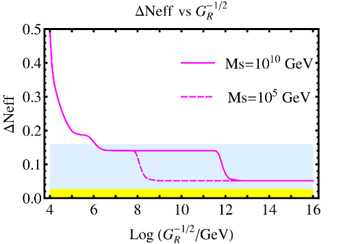
Suppose that CMB-S4 did not find new contributions and set an upper limit at 1 level. As shown in Fig(3), MSSM extension of DLRSM cannot save models of Dirac-type neutrinos. Nonetheless, Majorana-type neutrino models are acceptable. Similar arguments in SO(10) models [16] based on proliferated species of show that GUT scale of order GeV is acceptable to accommodate DLRSM structure. Thus, CMB-S4 is expected to have a great impact on physics beyond standard model.
V Combined analysis using summed neutrino mass measurement
Extra due to relic contributes to the summed neutrino masses, which is also a target of forthcoming CMB-S4 observations.
It is of great value to summarize analyzed data using the minimum neutrino mass value defined as . Neutrino oscillation data gives the summed neutrino mass in terms of different functions of , with different offset parameters in the normal hierarchical (NH) and the inverted hierarchical (IH) orderings;
| (27) |
for NH, and
| (28) |
for IH, where mass values are given in meV unit. We note that denotes the summed neutrino mass determined by cosmological observations. This quantity should be divided by the dilution factor to compare with the values of the oscillation experiments[15]. Offset values given by setting are and meV, for NH and IH, respectively. This difference in two ordering schemes is significantly large.
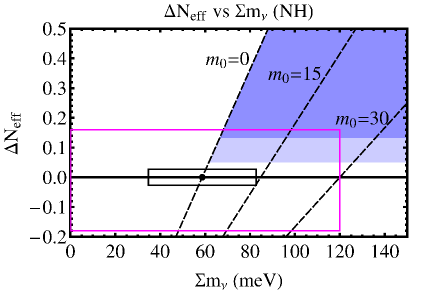
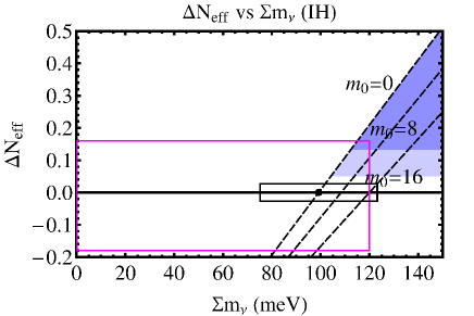
In Fig(4) we show the region in the plane allowed by Planck 2018 observations. These results hold irrespective of whether neutrinos are of Majorana or of Dirac type, since neutrino oscillation data cannot distinguish these two types. Nevertheless, plots given here can help NH and IH differences in future cosmological observations.
In the case of Dirac-type neutrino one can add more to this. One can readily convert to using (1) in favor of theoretical convenience of Dirac-type neutrino. We illustrate results in Fig(4) for three choices of the smallest neutrino mass. With improved accuracy in future observations one can reject IH schemes of larger smallest mass more readily than NH schemes. The minimum LR symmetric model is on the verge of rejection if IH scheme is adopted.
Considering these forecasts of cosmological observations, direct experiments of the smallest mass measurement and M/D distinction in terrestrial laboratories becomes even more important. It has been proposed to use laser-initiated coherence to measure these in atomic experiments in order to enhance otherwise tiny rates [18].
In summary, we investigated how cosmological observations of neutrino properties can probe still undetermined neutrino mass types and measure mass parameters with precision, under a few plausible assumptions: (1) three neutrino scheme, (2) zero chemical potential of thermal particles, (3) no hypothetical light relic or relics with small accumulated contribution to less than .
The Majorana neutrino, with rapid decay of its heavy right-handed partners, is in agreement with cosmological observations at nucleo-synthesis and at later epochs after recombination. But, Dirac-type right-handed neutrinos ’s, must be diluted away, to give , as limited by Planck + DESI observations. The necessary dilution is provided by rehearing left-handed neutrino after cosmological decoupling, hence the problem is sensitive to particle content in thermal equilibrium. It is necessary, for the answer to this question, to identify a proper theoretical framework of how right-handed neutrino bound is satisfied. We find it most natural to adopt gauge theories including SU(2)SU(2)U(1) as a subgroup, and how a nearly complete dilution of may occur, requiring a prolific set of particles as large as .
Implication of CMB-S4 sensitivity in Dirac-type neutrino models is that either SU(2)SU(2)U(1) is extended by supersymmetry allowing dilution after decoupling or grand unified extension of the left-right symmetric models is required as typical favored cases, thus making it possible to explore highest energy scale of particle physics.
The choice of NH or IH mass ordering scheme, irrespective of the mass types, should not be too difficult to determine in CMB-S4 observations.
Note added.
After completion of this work we became aware of the work, DESI Collaboration, arXiv:2404/03002v2[astro-ph[CO], in which analysis of DESI observations suggests that 72 meV is likely to be the upper bound of summed neutrino mass. This makes the right panel IH case in our Fig(4) disfavored.
Acknowledgements.
We appreciate O. Tajima at Kyoto University for valuable information and comments on CMB-S4 and other projects. This research was partially supported by Grant-in-Aid 19H00686 (NS), 18K03621 (MT), and 21K03575 (MY) from the Japanese Ministry of Education, Culture, Sports, Science, and Technology.Appendix A Doublet left-right symmetric model
A.1 Gauge symmetry and matter contents
The gauge symmetry of doublet left-right symmetric model (DLRSM) is
| (29) |
The fermions in DLRSM are
| (30) | |||
| (31) |
where gauge quantum numbers of underlying group are , , , , respectively for quarks , and leptons , .
Three types of scalars in DLRSM are introduced:
| (32) | |||
| (33) | |||
| (34) |
A.2 Spontaneous symmetry breaking (SSB)
The vacuum expectation values
| (35) | |||
| (36) | |||
| (37) |
with a fine-tuning inequality lead to the following SSB pattern:
| (38) |
The first step is relevant to the study of decoupling above the electroweak scale .
With a fine-tuning there is only one light Higgs boson of mass in the electroweak energy scale, while all other Higgs bosons remain much heavier than electroweak scale.
A.3 Nonstandard gauge bosons
In addition to the gauge bosons in the standard model, we have a pair of charged gauge bosons and a neutral gauge boson in the DLRSM. The mass eigenstates are expressed in terms of the gauge basis field as
| (39) | |||
| (40) | |||
| (41) |
where and are the gauge coupling constants of and respectively. Their masses are given by
| (42) |
Incidentally, the gauge boson is identified as the orthogonal state of as
| (43) |
and it is massless at this stage. With the gauge mixing angle defined by
| (44) |
one may express the neutral gauge bosons in the gauge basis in terms of those in the mass basis as
| (45) | |||
| (46) |
A.4 Nonstandard gauge interactions of fermions
The kinetic term of fermions is
| (47) |
with the covariant derivative given by
| (48) | |||||
where . The interaction is the one in the standard model with the left-handed fermions replaced by the right-handed ones. We find the interaction as
| (49) |
where
| (50) |
where , , , , and .
A.5 Gauge coupling constants
The nonstandard gauge coupling constants and are related to by
| (51) |
Thus, we cannot choose and independently. Assuming the manifest left-right symmetry , and taking and , we obtain and .
Appendix B Right-handed neutrino annihilation processes
Processes are listed in the text. We shall give amplitudes and squared amplitudes when relevant helicity states are added.
B.1 Amplitudes
B.1.1 t-channel exchange
| (52) | |||
| (53) |
where .
B.1.2 t-channel exchange
| (54) | |||
| (55) |
B.1.3 s-channel exchange ,
| (56) | |||
| (57) |
where , and .
B.1.4 s-channel exchange
| (58) |
B.2 Squared amplitudes
We evaluate , where means the average of initial spins and sum over final spins in spinor manipulation. It is straight forward to obtain the following squared fundamental amplitudes:
| (59) | |||
| (60) | |||
| (61) | |||
| (62) |
We also need the following interference term:
| (63) |
These results of helicity-summed squared amplitudes are checked by the software FeynCalc[19] as well.
B.3 Cross sections
The differential cross section is expressed by
| (64) |
where the two-body phase space is given by
| (65) | |||||
| (66) |
We have performed trivial parts of integration leaving the integration over variable. In the case of massless particles, and the range of integration is .
B.3.1 Right-handed neutrino pair annihilation process ,
| (67) |
In the four-Fermi approximation , using and (namely ), we find
| (68) |
B.3.2 Right-handed neutrino pair annihilation process ,
| (69) | |||||
| (70) |
where represents the number of colors.
B.3.3 Single right-handed neutrino annihilation process
| (71) | |||
| (72) |
B.3.4 Single right-handed neutrino annihilation process ,
| (73) | |||||
| (74) |
B.3.5 Single right-handed neutrino annihilation process
| (75) | |||
| (76) |
B.3.6 Total cross section
To summarize, the total annihilation cross section is given by
| (77) |
where , and represents the number of generations.
Appendix C Thermal average
We consider the thermal average of cross section times (Møller) velocity :
| (78) | |||
| (79) |
where , and denote the spin degrees of freedom, the number densities and the thermal distributions of the initial particles respectively. For the case of massless initial particles, we find and
| (81) | |||||
Relation of Fermi-Dirac (FD) and approximate Maxwell-Boltzmann (MB) distribution functions is .
C.1 Maxwell-Boltzmann approximation
for initial phase space integration
When the cross section is suppressed for smaller as in the case of the four-Fermi interaction, we expect that the Maxwell-Boltzmann distribution is a good approximation to the Fermi-Dirac distribution in the thermal average.
To evaluate the thermal integration, the following change of variables is convenient[20]:
| (82) |
where and the integration region is
| (83) |
for the massless case. With the Maxwell-Boltzmann distribution , we obtain (for the massless case)
| (84) |
where represents the modified Bessel function of the second kind.
C.1.1 Four-Fermi approximation
As explicitly shown in the previous section, the cross section is proportional to in the four-Fermi approximation. We find that the relevant thermal average is given by
| (85) |
and
| (86) |
C.2 Thermal average with Fermi-Dirac distribution
The relevant thermal average using Fermi-Dirac distribution function is
| (87) |
where
| (88) | |||||
| (89) |
Exchanging the order of and integrals, we obtain analytic result given in the text,
| (90) |
Then, we find
| (91) |
Appendix D Decoupling temperature
The right-handed neutrino annihilation rate is given by . We note that the factor of is introduced to compensate the initial spin average factor in the cross sections given in this appendix. In the four-Fermi and Maxwell-Boltzmann approximation, we obtain
| (92) |
With the Fermi-Dirac distribution, we find
| (93) |
It turns out that the the Maxwell-Boltzmann approximation is surprisingly accurate. To summarize,
| (94) |
where
| (95) |
The decoupling temperature is defined by
| (96) |
where is the Hubble constant and the Planck mass is . We note that for the standard model and in the present case.
In the four-Fermi approximation, the right-handed neutrino decoupling temperature is expressed by
| (97) |
References
- [1] P. Minkowski, Phys.Lett. B67, 421 (1977). The seesaw mechanism is presented in the SU(2)SU(2)U(1) framework. This important work has been overlooked in the literature, and the idea was resurrected by many others somewhat later.
- [2] M. Fukugita and T. Yanagida, Phys.Lett. B174, 45 (1986). This scenario utilizes sphaleron mediated process occurring in thermal medium at several to 10 TeV energy, which partially converts the generated lepton number to the baryon number.
- [3] The small contribution 0.046 due to neutrino spectrum distortion at non-instantaneous decoupling is found in G. Mangano, G. Miele, S. Pastor, T. Pinto, O. Pisanti, and P.S. Serpico, Nucl.Phys. B729, 221 (2005), arXiv:hep-ph/0506164 [hep-ph] and references therein, is ignored in the present work.
- [4] Planck collaboration, N. Aghanim et al., Planck 2018 results. VI. Cosmological parameters, arXiv: 1807.06209. Astron. Astrophys.641, A6 (2020)
- [5] K. N. Abazajian and J. Heeck, Phys. Rev. D100, 075027 (2019).
- [6] P. Adshead, Y. Cui, A.J. Long and M. Shamma, Phys. Lett. B823, 136736 (2021).
- [7] D. Borah, A. Dasgupta, C. Majumdar, D. Nanda, Phys.Rev. D102, 035025 (2020).
- [8] K.S. Babu, X-G. He, M. Su, and A. Thapa, JHEP 08, 140 (2022).
- [9] CMB-S4 Science Book, arXiv: 1610.02743v1[astro-ph.CO], (2016). Chapter 4 reviews the role of extra that receives contributions from light relics. In particular, Figure 29 of Section 4.4 summarizes BBN result, Planck 2015 result, and CMB-S4 expectations in the plane.
- [10] A.D. Dolgov, Physics Report, 370 333-535 (2002). See Section 6.4 in particular and references therein. Big-bang nucleo-synthesis (BBN) is briefly summarized in Section 3.4.
- [11] V. Bernard, S. Descotes-Genon, and L. Vale Silva, JHEP 09, 088 (2020). arXiv: 2001.00886[hep-ph]
- [12] S. Dimopoulos and H. Georgi, Nuclear Physics B. 193, 150 (1981). S. Dimopoulos, S. Raby, and F. Wilczek, Physical Review D. 24, 1681 (1981).
- [13] For an overview of MSSM, see Perspectives on Supersymmetry II, Edited By: Gordon L Kane, World Scientific Publishing, Singapore (2010).
- [14] C.S. Aulakh, B. Bajc, A. Melfo, G. Senjanovic, and F. Vissani, Phys.Lett.B 588, 196 (2004). B. Bajc, A. Melfo, G. Senjanovic, and F. Vissani, Phys.Lett.B 634, 272 (2006).
- [15] I, Esteban, M.C. Gonzalez-Garcia, M. Maltoni, T. Schwetz, and A. Zhou, The fate of hints: updated global analysis of three-flavor neutrino oscillations, JHEP 09, 178 (2020); arXiv: 2007.14792 [hep-ph]
- [16] K.S. Babu and R.N. Mohapatra, Phys. Rev. Lett. 70, 2845 (1993), and references therein. This model incorporates the seesaw mass generation due to heavy Majorana neutrinos. We assume that a modification of Higgs potential can lead to the Dirac-type neutrino.
- [17] R. Allison, P. Caucal, E. Calabrese, J. Dunkley, and T. Louis, Phys. Rev. D92, 123535 (2015). Towards a cosmological neutrino mass detection, arXiv: 1509.07471 (2015).
- [18] A. Fukumi, et al, PTEP 2012, 04D002 (2012): e-Print: 1211.4904 [hep-ph]. M. Yoshimura, N. Sasao, and M. Tanaka, Phys.Rev.D91, 063516 (2015): Experimental method of detecting relic neutrino by atomic de-excitation arXiv: 1409.3648[hep-ph]. H. Hara, A. Yoshimi, and M. Yoshimura, Phys.Rev. D104, 115006 (2021). arXiv: 2105.11114 [hep-ph] and references therein.
- [19] V. Shtabovenko, R. Mertig and F. Orellana, Comput. Phys. Commun., 207, 432-444, 2016, arXiv:1601.01167. ”FeynCalc 9.3: New features and improvements”, arXiv:2001.04407.
- [20] P. Gondolo and G. Gelmini, Nucl. Phys. B360, 145 (1991).