This paper was converted on www.awesomepapers.org from LaTeX by an anonymous user.
Want to know more? Visit the Converter page.

Implication of Kπνν¯K\to\pi\nu\bar{\nu} for generic neutrino interactions in effective field theories

Tong Li [email protected] School of Physics, Nankai University, Tianjin 300071, China    Xiao-Dong Ma [email protected] Department of Physics, National Taiwan University, Taipei 10617, Taiwan    Michael A. Schmidt [email protected] School of Physics, The University of New South Wales, Sydney, New South Wales 2052, Australia
Abstract

In this work we investigate the implication of Kπνν¯K\to\pi\nu\bar{\nu} from the recent KOTO and NA62 measurements for generic neutrino interactions and the new physics scale in effective field theories. The interactions between quarks and left-handed Standard Model (SM) neutrinos are first described by the low energy effective field theory (LEFT) below the electroweak scale. We match them to the chiral perturbation theory (χ\chiPT) at the chiral symmetry breaking scale to calculate the branching fractions of Kaon semi-invisible decays and match them up to the SM effective field theory (SMEFT) to constrain new physics above the electroweak scale. In the framework of effective field theories, we prove that the Grossman-Nir bound is valid for both dim-6 and dim-7 LEFT operators, and the dim-6 vector and scalar operators dominantly contribute to Kaon semi-invisible decays based on LEFT and chiral power counting rules. They are induced by multiple dim-6 lepton-number-conserving operators and one dim-7 lepton-number-violating operator in the SMEFT, respectively. In the lepton-number-conserving sds\to d transition, the Kπνν¯K\to\pi\nu\bar{\nu} decays provide the most sensitive probe for the operators with ττ\tau\tau component and point to a corresponding new physics scale of ΛNP[47TeV,72TeV]\Lambda_{\rm NP}\in[47~{}\text{TeV},~{}72~{}\text{TeV}] associated with a single effective coefficient. The lepton-number-violating operator can also explain the observed Kπνν¯K\to\pi\nu\bar{\nu} discrepancy with the SM prediction within a narrow range ΛNP[19.4TeV,21.5TeV]\Lambda_{\rm NP}\in[19.4~{}\text{TeV},~{}21.5~{}\text{TeV}], which is consistent with constraints from Kaon invisible decays.

I Introduction

Recently, the KOTO experiment at J-PARC Shinohara ; Lin and the NA62 experiment at CERN Ruggiero announced preliminary results of Kaon semi-invisible decays Kitahara et al. (2019)

KLπ0νν¯KOTO16/18\displaystyle{\mathcal{B}}_{K_{L}\to\pi^{0}\nu\bar{\nu}}^{\text{KOTO16/18}} =\displaystyle= 2.11.7+4.1×10⁹,\displaystyle 2.1^{+4.1}_{-1.7}\times 10^{-9}, (1)
K+π+νν¯NA62\displaystyle{\mathcal{B}}_{K^{+}\to\pi^{+}\nu\bar{\nu}}^{\text{NA62}} <\displaystyle< 2.44×10¹⁰,\displaystyle 2.44\times 10^{-10}, (2)

at the 95% confidence level (CL). They update the upper limit on the decay rate of K+π+νν¯K^{+}\to\pi^{+}\nu\bar{\nu} from BNL E949 Artamonov et al. (2008, 2009) and the limit on the branching ratio (KLπ0νν¯){\mathcal{B}}(K_{L}\to\pi^{0}\nu\bar{\nu}) from the 2015 run at KOTO itself Ahn et al. (2019)

KLπ0νν¯KOTO15\displaystyle{\mathcal{B}}_{K_{L}\to\pi^{0}\nu\bar{\nu}}^{\text{KOTO15}} <\displaystyle< 3.0×10⁹,\displaystyle 3.0\times 10^{-9}, (3)
K+π+νν¯E949\displaystyle{\mathcal{B}}_{K^{+}\to\pi^{+}\nu\bar{\nu}}^{E949} <\displaystyle< 3.35×10¹⁰,\displaystyle 3.35\times 10^{-10}, (4)

at the 90% CL. These decays are mediated by flavor changing neutral currents (FCNC) and thus are suppressed by the GIM mechanism in the Standard Model (SM), giving KLπ0νν¯SM=(3.4±0.6)×1011{\mathcal{B}}_{K_{L}\to\pi^{0}\nu\bar{\nu}}^{\text{SM}}=(3.4\pm 0.6)\times 10^{-11} and K+π+νν¯SM=(8.4±1.0)×1011{\mathcal{B}}_{K^{+}\to\pi^{+}\nu\bar{\nu}}^{\text{SM}}=(8.4\pm 1.0)\times 10^{-11}, respectively Buras et al. (2006); Brod et al. (2011); Buras et al. (2015). In the SM no events are expected from the above Kaon rare decays, but KOTO reported three signal events in the search of KLπ0νν¯K_{L}\to\pi^{0}\nu\bar{\nu}. There exist quite a few works trying to explain these intriguing events reported by KOTO Kitahara et al. (2019); Fabbrichesi and Gabrielli (2019); Egana-Ugrinovic et al. (2019); Dev et al. (2019) (or constrain particular new physics (NP) models Fuyuto et al. (2015); Mandal and Pich (2019); Calibbi et al. (2019)) and meanwhile avoid the violation of its relation with the K+π+νν¯K^{+}\to\pi^{+}\nu\bar{\nu} decay, that is the Grossman-Nir bound Grossman and Nir (1997). These efforts require the introduction of a new invisible degree of freedom with the mass scale being around 100200100-200 MeV.

The interpretation of the KOTO result depends on not only whether the invisible particles are viewed as neutrinos, but also the experimental uncertainties. Even if we only take into account the statistical uncertainties at 95% CL for neutrino final states, there is allowed space for heavy NP beyond the SM consistent with both KLπ0νν¯K_{L}\to\pi^{0}\nu\bar{\nu} and K+π+νν¯K^{+}\to\pi^{+}\nu\bar{\nu} measurements and satisfying the Grossman-Nir bound. As one can see from the Fig. 1 in Ref. Kitahara et al. (2019), the allowed region is rather delimited and not far away from the SM prediction. It can provide a constraint on the relevant quark-neutrino interactions and shed light on the search for generic neutrino interactions in the future. Thus, without introducing any new light particles, we focus on heavy NP contributing to the generic quark-neutrino interactions and generically confine the NP scale from the allowed region of (KLπ0νν¯){\mathcal{B}}(K_{L}\to\pi^{0}\nu\bar{\nu}) and (K+π+νν¯){\mathcal{B}}(K^{+}\to\pi^{+}\nu\bar{\nu}) measurements. As the neutrino flavor is not measured and the fermionic nature of neutrinos is not determined, the semi-invisible Kaon decays Kπνν¯K\to\pi\nu\bar{\nu} are sensitive probes for a range of interactions.

In this work, we will use an effective field theory approach, where NP is described by a set of non-renormalizable operators which are added to the SM Lagrangian

eff=SM+id5Ci(d)𝒪i(d).\displaystyle\mathcal{L}_{\rm eff}=\mathcal{L}_{\rm SM}+\sum_{i}\sum_{d\geq 5}C_{i}^{(d)}{\mathcal{O}}_{i}^{(d)}\;. (5)

Here 𝒪i(d){\mathcal{O}}_{i}^{(d)} are the dimension-dd (dim-dd in short below) effective operators. Each Wilson coefficient Ci(d)C_{i}^{(d)} is associated with a NP scale ΛNP=(Ci(d))1/(4d)\Lambda_{\rm NP}=(C_{i}^{(d)})^{1/(4-d)}. We first use the low energy effective field theory (LEFT) Jenkins et al. (2018a, b) to describe the interactions between quarks and left-handed SM neutrinos below the electroweak scale. Then, in order to calculate the Kaon decay rate, we match the LEFT operators to chiral perturbation theory (χ\chiPT) Gasser and Leutwyler (1984, 1985) at the chiral symmetry breaking scale to take into account non-perturbative QCD effects. The branching fractions of Kaon semi-invisible decays are evaluated in terms of the Wilson coefficients and neutrino bilinears as external sources. Finally, we match them up to the Standard Model effective field theory (SMEFT) to constrain new physics above the electroweak scale Buchmuller and Wyler (1986); Grzadkowski et al. (2010); Lehman (2014); Liao and Ma (2016); Henning et al. (2017); Liao and Ma (2017).

The paper is outlined as follows. In Sec. II, we describe the LEFT basis and give the quark-neutrino operators relevant for our study. The LEFT operators are matched to χ\chiPT and we show the general expressions for the branching fractions of Kaon semi-invisible decays. We then match the results to the SMEFT in Sec. III. In Sec. IV we show the implication of Kπνν¯K\to\pi\nu\bar{\nu} for new physics and discuss other constraints. Our conclusions and some discussions are drawn in Sec. V. Some calculation details for Kaon decays are collected in the Appendix.

II Generic neutrino interactions and Kπνν¯K\to\pi\nu\bar{\nu} calculation in χ\chiPT

II.1 Generic quark-neutrino operators in LEFT basis

We consider the effective operators for neutrino bilinears coupled to SM quarks in the framework of LEFT obeying SU(3)c×(3)_{\rm c}\timesU(1)em(1)_{\rm em} gauge symmetry. In the basis of LEFT for neutrinos, the only dim-5 operator contributing to the neutrino magnetic moments is Canas et al. (2016)

𝒪ννF\displaystyle{\mathcal{O}}_{\nu\nu F} =\displaystyle= (νC¯iσμνν)Fμν+h.c.,\displaystyle(\overline{\nu^{C}}i\sigma_{\mu\nu}\nu)F^{\mu\nu}+h.c.\;, (6)

where FμνF_{\mu\nu} is the electromagnetic field strength tensor and ν=PLν\nu=P_{L}\nu denote left-handed active SM neutrinos. Its SMEFT completion has been investigated by Cirigliano et al. in Ref. Cirigliano et al. (2017). In principle, the neutrino magnetic moment operator can yield the KπννK\to\pi\nu\nu process through a long-distance contribution with one vertex connecting to the sdγs\to d\gamma transition operator s¯σμνPL/RdFμν\bar{s}\sigma_{\mu\nu}P_{L/R}dF^{\mu\nu}. The corresponding coefficient is estimated to be CsdF109GeV1C_{sdF}\sim 10^{-9}~{}{\rm GeV}^{-1} in the SM Tandean (2000). There also exists a strong constraint on |CννF|4×10⁹GeV1|C_{\nu\nu F}|\leq 4\times 10^{-9}~{}{\rm GeV}^{-1} Canas et al. (2016). We thus conclude that the contribution from this operator to KπννK\to\pi\nu\nu transition is negligible. There are also the dim-6 operators Jenkins et al. (2018a) with lepton number conservation (LNC, |ΔL|=0|\Delta L|=0)

𝒪uν1V\displaystyle{\mathcal{O}}_{u\nu 1}^{V} =(uL¯γμuL)(ν¯γμν),\displaystyle=(\overline{u_{L}}\gamma^{\mu}u_{L})(\overline{\nu}\gamma^{\mu}\nu)\;, 𝒪dν1V\displaystyle{\mathcal{O}}_{d\nu 1}^{V} =(dL¯γμdL)(ν¯γμν),\displaystyle=(\overline{d_{L}}\gamma^{\mu}d_{L})(\overline{\nu}\gamma^{\mu}\nu)\;, (7)
𝒪uν2V\displaystyle{\mathcal{O}}_{u\nu 2}^{V} =(uR¯γμuR)(ν¯γμν),\displaystyle=(\overline{u_{R}}\gamma^{\mu}u_{R})(\overline{\nu}\gamma^{\mu}\nu)\;, 𝒪dν2V\displaystyle{\mathcal{O}}_{d\nu 2}^{V} =(dR¯γμdR)(ν¯γμν),\displaystyle=(\overline{d_{R}}\gamma^{\mu}d_{R})(\overline{\nu}\gamma^{\mu}\nu)\;, (8)

and those with lepton number violation (LNV, |ΔL|=2|\Delta L|=2)

𝒪uν1S\displaystyle{\mathcal{O}}_{u\nu 1}^{S} =(uR¯uL)(νC¯ν)+h.c.,\displaystyle=(\overline{u_{R}}u_{L})(\overline{\nu^{C}}\nu)+h.c.\;, 𝒪dν1S\displaystyle{\mathcal{O}}_{d\nu 1}^{S} =(dR¯dL)(νC¯ν)+h.c.,\displaystyle=(\overline{d_{R}}d_{L})(\overline{\nu^{C}}\nu)+h.c.\;, (9)
𝒪uν2S\displaystyle{\mathcal{O}}_{u\nu 2}^{S} =(uL¯uR)(νC¯ν)+h.c.,\displaystyle=(\overline{u_{L}}u_{R})(\overline{\nu^{C}}\nu)+h.c.\;, 𝒪dν2S\displaystyle{\mathcal{O}}_{d\nu 2}^{S} =(dL¯dR)(νC¯ν)+h.c.,\displaystyle=(\overline{d_{L}}d_{R})(\overline{\nu^{C}}\nu)+h.c.\;, (10)
𝒪uνT\displaystyle{\mathcal{O}}_{u\nu}^{T} =(uR¯σμνuL)(νC¯σμνν)+h.c.,\displaystyle=(\overline{u_{R}}\sigma^{\mu\nu}u_{L})(\overline{\nu^{C}}\sigma_{\mu\nu}\nu)+h.c.\;, 𝒪dνT\displaystyle{\mathcal{O}}_{d\nu}^{T} =(dR¯σμνdL)(νC¯σμνν)+h.c..\displaystyle=(\overline{d_{R}}\sigma^{\mu\nu}d_{L})(\overline{\nu^{C}}\sigma_{\mu\nu}\nu)+h.c.\;. (11)

where uL(uR)u_{L}(u_{R}) and dL(dR)d_{L}(d_{R}) denote the left- (right-) handed up-type and down-type quark fields in mass basis, respectively. Note that the tensor operator ναC¯σμννβ\overline{\nu_{\alpha}^{C}}\sigma^{\mu\nu}\nu_{\beta} vanishes for identical neutrino flavors (with α=β\alpha=\beta). The flavors of the two quarks and those of the two neutrinos in the above operators can be different although we do not specify their flavor indexes here. For the notation of the Wilson coefficients, we use the same subscripts as the operators, for instance Cdν1V,xyαβC_{d\nu 1}^{V,xy\alpha\beta} together with 𝒪dν1V,xyαβ{\mathcal{O}}_{d\nu 1}^{V,xy\alpha\beta}, where x,yx,y denote the down-type quark flavors and α,β\alpha,\beta are the neutrino flavors. In the following we will study the KπK\to\pi transition and thus only consider the operators with down-type quarks ss and dd.

II.2 Matching to the leading order of χ\chiPT

The dim-6 quark-neutrino operators can be matched onto the meson-lepton interactions through the χ\chiPT formalism by treating the lepton currents together with the accompanied Wilson coefficients as proper external sources. The QCD-like Lagrangian with external sources for the first three light quarks (q=u,d,sq=u,d,s) can be described as

QCD=QCDmq=0+qL¯lμγμqL+qR¯rμγμqR+[qL¯(sip)qR+qL¯(tlμνσμν)qR+h.c.],\displaystyle\mathcal{L}_{\rm QCD}=\mathcal{L}_{\text{QCD}}^{m_{q}=0}+\overline{q_{L}}l_{\mu}\gamma^{\mu}q_{L}+\overline{q_{R}}r_{\mu}\gamma^{\mu}q_{R}+\left[\overline{q_{L}}(s-ip)q_{R}+\overline{q_{L}}(t_{l}^{\mu\nu}\sigma_{\mu\nu})q_{R}+h.c.\right], (12)

where the flavor space 3×3\times3 matrices {lμ=lμ,rμ=rμ,s=s,p=p,trμν=tlμν}\{l_{\mu}=l_{\mu}^{\dagger},~{}r_{\mu}=r_{\mu}^{\dagger},~{}s=s^{\dagger},~{}p=p^{\dagger},~{}t_{r}^{\mu\nu}=t_{l}^{\mu\nu\dagger}\} are the external sources related with the corresponding quark currents. One can extract the relevant external sources from the above dim-6 effective operators. On the other hand, based on Weinberg’s power-counting scheme, the most general chiral Lagrangian can be expanded according to the momentum pp and quark mass. The chiral Lagrangian with external sources at leading order reads Gasser and Leutwyler (1984, 1985)

p2=F024Tr(DμU(DμU))+F024Tr(χU+Uχ),\displaystyle\mathcal{L}_{p^{2}}=\frac{F_{0}^{2}}{4}{{\rm Tr}}\left(D_{\mu}U(D^{\mu}U)^{\dagger}\right)+\frac{F_{0}^{2}}{4}{{\rm Tr}}\left(\chi U^{\dagger}+U\chi^{\dagger}\right), (13)

where UU is the standard matrix for the Nambu-Goldstone bosons

U=exp(iΦF0),Φ=(π0+η32π+2K+2ππ0+η32K02K2K¯023η),\displaystyle U={\rm exp}\Big{(}{i\Phi\over F_{0}}\Big{)},\ \ \Phi=\left(\begin{array}[]{ccc}\pi^{0}+{\eta\over\sqrt{3}}&\sqrt{2}\pi^{+}&\sqrt{2}K^{+}\\ \sqrt{2}\pi^{-}&-\pi^{0}+{\eta\over\sqrt{3}}&\sqrt{2}K^{0}\\ \sqrt{2}K^{-}&\sqrt{2}\bar{K}^{0}&-{2\over\sqrt{3}}\eta\\ \end{array}\right)\;, (17)

with the constant F0F_{0} being referred to the pion decay constant in the chiral limit. The covariant derivative of UU and χ\chi are expressed in terms of the external sources

DμU\displaystyle D_{\mu}U =μUilμU+iUrμ,\displaystyle=\partial_{\mu}U-il_{\mu}U+iUr_{\mu}, χ\displaystyle\chi =2B(sip),\displaystyle=2B(s-ip), χ\displaystyle\chi^{\dagger} =2B(s+ip),\displaystyle=2B(s+ip), (18)

where the constant BB is related to the quark condensate and F0F_{0} by B=q¯q0/(3F02)B=-\langle\bar{q}q\rangle_{0}/(3F_{0}^{2}). For the later numerical estimation, we take F0=87MeVF_{0}=87~{}\text{MeV} Colangelo and Durr (2004) and B2.8GeVB\approx 2.8~{}\text{GeV} Cirigliano et al. (2017); Patrignani et al. (2016). The Nambu-Goldstone bosons parameterized by UU and the (pseudo-)scalar sources χ\chi transform as ULURU\to LUR^{\dagger} and χLχR\chi\to L\chi R^{\dagger}, where LL (RR) is SU(3)LSU(3)_{L} (SU(3)RSU(3)_{R}) transformation.

By inspecting the dim-6 operators related to the sdνν^s\rightarrow d\nu\widehat{\nu} transition (the symbol  ‘ ^\widehat{} ’  here indicating the neutrino pair can be either LNC νν¯\nu\bar{\nu} or LNV νν\nu\nu111Below we use Kπνν¯K\to\pi\nu\bar{\nu} to generally denote the experimental processes. Kπνν^K\to\pi\nu\widehat{\nu} appears when both νν¯\nu\bar{\nu} and νν\nu\nu final states can occur in the analytical expressions of the theoretical calculation unless a LNC or LNV process is specified in our discussion.), we find that only the LNC operators 𝒪dν1V,𝒪dν2V{\mathcal{O}}_{d\nu 1}^{V},~{}{\mathcal{O}}_{d\nu 2}^{V} and LNV operators 𝒪dν1S,𝒪dν2S{\mathcal{O}}_{d\nu 1}^{S},~{}{\mathcal{O}}_{d\nu 2}^{S} can contribute to the leading order chiral Lagrangian. The tensor operator 𝒪dνT{\mathcal{O}}_{d\nu}^{T} only contributes to the next-to-leading order chiral Lagrangian at 𝒪(p4)\mathcal{O}(p^{4}). They lead to the following external sources

(lμ)sd\displaystyle(l^{\mu})_{sd} =\displaystyle= Cdν1V,sdαβ(να¯γμνβ),\displaystyle C_{d\nu 1}^{V,sd\alpha\beta}(\overline{\nu_{\alpha}}\gamma^{\mu}\nu_{\beta}), (19)
(lμ)ds\displaystyle(l^{\mu})_{ds} =\displaystyle= Cdν1V,dsαβ(να¯γμνβ),\displaystyle C_{d\nu 1}^{V,ds\alpha\beta}(\overline{\nu_{\alpha}}\gamma^{\mu}\nu_{\beta}), (20)
(rμ)sd\displaystyle(r^{\mu})_{sd} =\displaystyle= Cdν2V,sdαβ(να¯γμνβ),\displaystyle C_{d\nu 2}^{V,sd\alpha\beta}(\overline{\nu_{\alpha}}\gamma^{\mu}\nu_{\beta}), (21)
(rμ)ds\displaystyle(r^{\mu})_{ds} =\displaystyle= Cdν2V,dsαβ(να¯γμνβ),\displaystyle C_{d\nu 2}^{V,ds\alpha\beta}(\overline{\nu_{\alpha}}\gamma^{\mu}\nu_{\beta}), (22)
(s+ip)sd\displaystyle(s+ip)_{sd} =\displaystyle= Cdν1S,sdαβ(ναC¯νβ)+Cdν2S,dsαβ(να¯νβC),\displaystyle C_{d\nu 1}^{S,sd\alpha\beta}(\overline{\nu^{C}_{\alpha}}\nu_{\beta})+C_{d\nu 2}^{S,ds\alpha\beta*}(\overline{\nu_{\alpha}}\nu_{\beta}^{C}), (23)
(s+ip)ds\displaystyle(s+ip)_{ds} =\displaystyle= Cdν1S,dsαβ(ναC¯νβ)+Cdν2S,sdαβ(να¯νβC),\displaystyle C_{d\nu 1}^{S,ds\alpha\beta}(\overline{\nu^{C}_{\alpha}}\nu_{\beta})+C_{d\nu 2}^{S,sd\alpha\beta*}(\overline{\nu_{\alpha}}\nu_{\beta}^{C}), (24)
(sip)sd\displaystyle(s-ip)_{sd} =\displaystyle= Cdν1S,dsαβ(να¯νβC)+Cdν2S,sdαβ(ναC¯νβ),\displaystyle C_{d\nu 1}^{S,ds\alpha\beta*}(\overline{\nu_{\alpha}}\nu_{\beta}^{C})+C_{d\nu 2}^{S,sd\alpha\beta}(\overline{\nu^{C}_{\alpha}}\nu_{\beta}), (25)
(sip)ds\displaystyle(s-ip)_{ds} =\displaystyle= Cdν1S,sdαβ(να¯νβC)+Cdν2S,dsαβ(ναC¯νβ).\displaystyle C_{d\nu 1}^{S,sd\alpha\beta*}(\overline{\nu_{\alpha}}\nu_{\beta}^{C})+C_{d\nu 2}^{S,ds\alpha\beta}(\overline{\nu^{C}_{\alpha}}\nu_{\beta}). (26)

After expanding UU, i.e. U=1+iΦF0+12F02(iΦ)2+U=1+i{\Phi\over F_{0}}+{1\over 2F_{0}^{2}}(i\Phi)^{2}+\cdots and the insertion of the above external sources into the Lagrangian in Eq. (13), we obtain the effective Lagrangians for K0π0νν^K^{0}\to\pi^{0}\nu\widehat{\nu} and K+π+νν^K^{+}\to\pi^{+}\nu\widehat{\nu} at the leading order

K0π0νν^\displaystyle\mathcal{L}_{K^{0}\to\pi^{0}\nu\widehat{\nu}} =\displaystyle= B22[(Cdν1S,sdαβ+Cdν2S,sdαβ)(ναC¯νβ)+(Cdν1S,dsαβ+Cdν2S,dsαβ)(να¯νβC)]K0π0\displaystyle{B\over 2\sqrt{2}}\Big{[}\left(C_{d\nu 1}^{S,sd\alpha\beta}+C_{d\nu 2}^{S,sd\alpha\beta}\right)(\overline{\nu^{C}_{\alpha}}\nu_{\beta})+\left(C_{d\nu 1}^{S,ds\alpha\beta*}+C_{d\nu 2}^{S,ds\alpha\beta*}\right)(\overline{\nu_{\alpha}}\nu_{\beta}^{C})\Big{]}K^{0}\pi^{0} (27)
i22(Cdν1V,sdαβ+Cdν2V,sdαβ)(να¯γμνβ)(K0μπ0μK0π0),\displaystyle-{i\over 2\sqrt{2}}\left(C_{d\nu 1}^{V,sd\alpha\beta}+C_{d\nu 2}^{V,sd\alpha\beta}\right)(\overline{\nu_{\alpha}}\gamma^{\mu}\nu_{\beta})(K^{0}\partial_{\mu}\pi^{0}-\partial_{\mu}K^{0}\pi^{0})\;,
K+π+νν^\displaystyle\mathcal{L}_{K^{+}\to\pi^{+}\nu\widehat{\nu}} =\displaystyle= B2[(Cdν1S,sdαβ+Cdν2S,sdαβ)(ναC¯νβ)+(Cdν1S,dsαβ+Cdν2S,dsαβ)(να¯νβC)]K+π\displaystyle-{B\over 2}\Big{[}\left(C_{d\nu 1}^{S,sd\alpha\beta}+C_{d\nu 2}^{S,sd\alpha\beta}\right)(\overline{\nu^{C}_{\alpha}}\nu_{\beta})+\left(C_{d\nu 1}^{S,ds\alpha\beta*}+C_{d\nu 2}^{S,ds\alpha\beta*}\right)(\overline{\nu_{\alpha}}\nu_{\beta}^{C})\Big{]}K^{+}\pi^{-} (28)
+i2(Cdν1V,sdαβ+Cdν2V,sdαβ)(να¯γμνβ)(K+μπμK+π).\displaystyle+{i\over 2}\left(C_{d\nu 1}^{V,sd\alpha\beta}+C_{d\nu 2}^{V,sd\alpha\beta}\right)(\overline{\nu_{\alpha}}\gamma^{\mu}\nu_{\beta})(K^{+}\partial_{\mu}\pi^{-}-\partial_{\mu}K^{+}\pi^{-})\;.

The above Lagrangians fit to the relation

π0|K0π0νν^|K0π|K+π+νν^|K+=12.\displaystyle{\langle\pi^{0}|\mathcal{L}_{K^{0}\to\pi^{0}\nu\widehat{\nu}}|K^{0}\rangle\over\langle\pi^{-}|\mathcal{L}_{K^{+}\to\pi^{+}\nu\widehat{\nu}}|K^{+}\rangle}=-\frac{1}{\sqrt{2}}\;. (29)

This relation is the result of the transition operators that change isospin by 1/21/2. By neglecting the small CP violation in K0K¯0K^{0}-\bar{K}^{0} mixing, for the KLπ0K_{L}\rightarrow\pi^{0} transition, the relevant effective Lagrangian becomes

KLπ0νν^\displaystyle\mathcal{L}_{K_{L}\to\pi^{0}\nu\widehat{\nu}} =\displaystyle= B4[(Cdν1S,sdαβ+Cdν2S,sdαβ+Cdν1S,dsαβ+Cdν2S,dsαβ)(ναC¯νβ)\displaystyle{B\over 4}\Big{[}\left(C_{d\nu 1}^{S,sd\alpha\beta}+C_{d\nu 2}^{S,sd\alpha\beta}+C_{d\nu 1}^{S,ds\alpha\beta}+C_{d\nu 2}^{S,ds\alpha\beta}\right)(\overline{\nu^{C}_{\alpha}}\nu_{\beta})
+(Cdν1S,dsαβ+Cdν2S,dsαβ+Cdν1S,sdαβ+Cdν2S,sdαβ)(να¯νβC)]KLπ0\displaystyle+\left(C_{d\nu 1}^{S,ds\alpha\beta*}+C_{d\nu 2}^{S,ds\alpha\beta*}+C_{d\nu 1}^{S,sd\alpha\beta*}+C_{d\nu 2}^{S,sd\alpha\beta*}\right)(\overline{\nu_{\alpha}}\nu_{\beta}^{C})\Big{]}K_{L}\pi^{0}
i4(Cdν1V,sdαβ+Cdν2V,sdαβCdν1V,dsαβCdν2V,dsαβ)(να¯γμνβ)(KLμπ0μKLπ0),\displaystyle-{i\over 4}\left(C_{d\nu 1}^{V,sd\alpha\beta}+C_{d\nu 2}^{V,sd\alpha\beta}-C_{d\nu 1}^{V,ds\alpha\beta}-C_{d\nu 2}^{V,ds\alpha\beta}\right)(\overline{\nu_{\alpha}}\gamma^{\mu}\nu_{\beta})(K_{L}\partial_{\mu}\pi^{0}-\partial_{\mu}K_{L}\pi^{0})\;,

where the flavor indices α,β\alpha,\beta are summed over all three neutrino generations. Note that the Wilson coefficients for the scalar operators are symmetric in the neutrino flavor indices. From the effective Lagrangian we derive the branching ratios for the decays KLπ0νν^K_{L}\to\pi^{0}\nu\widehat{\nu} and K+π+νν^K^{+}\to\pi^{+}\nu\widehat{\nu}

KLπ0νν^\displaystyle\mathcal{B}_{K_{L}\rightarrow\pi^{0}\nu\widehat{\nu}} =\displaystyle= J1KLαβ(112δαβ)|Cdν1S,sdαβ+Cdν2S,sdαβ+Cdν1S,dsαβ+Cdν2S,dsαβ|2\displaystyle J_{1}^{K_{L}}\sum_{\alpha\leq\beta}\left(1-{1\over 2}\delta_{\alpha\beta}\right)\left|C_{d\nu 1}^{S,sd\alpha\beta}+C_{d\nu 2}^{S,sd\alpha\beta}+C_{d\nu 1}^{S,ds\alpha\beta}+C_{d\nu 2}^{S,ds\alpha\beta}\right|^{2} (31)
+J2KLα,β|Cdν1V,sdαβ+Cdν2V,sdαβCdν1V,dsαβCdν2V,dsαβ|2,\displaystyle+J_{2}^{K_{L}}\sum_{\alpha,\beta}\left|C_{d\nu 1}^{V,sd\alpha\beta}+C_{d\nu 2}^{V,sd\alpha\beta}-C_{d\nu 1}^{V,ds\alpha\beta}-C_{d\nu 2}^{V,ds\alpha\beta}\right|^{2},
K+π+νν^\displaystyle\mathcal{B}_{K^{+}\rightarrow\pi^{+}\nu\widehat{\nu}} =\displaystyle= J1K+αβ(112δαβ)(|Cdν1S,sdαβ+Cdν2S,sdαβ|2+|Cdν1S,dsαβ+Cdν2S,dsαβ|2)\displaystyle J_{1}^{K^{+}}\sum_{\alpha\leq\beta}\left(1-{1\over 2}\delta_{\alpha\beta}\right)\left(\left|C_{d\nu 1}^{S,sd\alpha\beta}+C_{d\nu 2}^{S,sd\alpha\beta}\right|^{2}+\left|C_{d\nu 1}^{S,ds\alpha\beta}+C_{d\nu 2}^{S,ds\alpha\beta}\right|^{2}\right) (32)
+J2K+α,β|Cdν1V,sdαβ+Cdν2V,sdαβ|2.\displaystyle+J_{2}^{K^{+}}\sum_{\alpha,\beta}\left|C_{d\nu 1}^{V,sd\alpha\beta}+C_{d\nu 2}^{V,sd\alpha\beta}\right|^{2}.

The details of the calculation are collected in Appendix A. The JJ functions parameterize the kinematics of the three-body decay and are defined as

J1KL\displaystyle J_{1}^{K_{L}} =\displaystyle= 1ΓKLExpB229π3mKL3𝑑ss((mKL2+mπ02s)24mKL2mπ02)1/2=40.4GF2,\displaystyle{1\over\Gamma_{K_{L}}^{\text{Exp}}}{B^{2}\over 2^{9}\pi^{3}m_{K_{L}}^{3}}\int ds\,s\left((m_{K_{L}}^{2}+m_{\pi^{0}}^{2}-s)^{2}-4m_{K_{L}}^{2}m_{\pi^{0}}^{2}\right)^{1/2}=40.4G_{F}^{-2}, (33)
J2KL\displaystyle J_{2}^{K_{L}} =\displaystyle= 1ΓKLExp13211π3mKL3𝑑s((mKL2+mπ02s)24mKL2mπ02)3/2=0.247GF2,\displaystyle{1\over\Gamma_{K_{L}}^{\text{Exp}}}{1\over 3\cdot 2^{11}\pi^{3}m_{K_{L}}^{3}}\int ds\left((m_{K_{L}}^{2}+m_{\pi^{0}}^{2}-s)^{2}-4m_{K_{L}}^{2}m_{\pi^{0}}^{2}\right)^{3/2}=0.247G_{F}^{-2}, (34)
J1K+\displaystyle J_{1}^{K^{+}} =\displaystyle= 1ΓK+ExpB228π3mK+3𝑑ss((mK+2+mπ+2s)24mK+2mπ+2)1/2=17.9GF2,\displaystyle{1\over\Gamma_{K^{+}}^{\text{Exp}}}{B^{2}\over 2^{8}\pi^{3}m_{K^{+}}^{3}}\int ds\,s\left((m_{K^{+}}^{2}+m_{\pi^{+}}^{2}-s)^{2}-4m_{K^{+}}^{2}m_{\pi^{+}}^{2}\right)^{1/2}=17.9G_{F}^{-2}, (35)
J2K+\displaystyle J_{2}^{K^{+}} =\displaystyle= 1ΓK+Exp1329π3mK+3𝑑s((mK+2+mπ+2s)24mK+2mπ+2)3/2=0.22GF2,\displaystyle{1\over\Gamma_{K^{+}}^{\text{Exp}}}{1\over 3\cdot 2^{9}\pi^{3}m_{K^{+}}^{3}}\int ds\left((m_{K^{+}}^{2}+m_{\pi^{+}}^{2}-s)^{2}-4m_{K^{+}}^{2}m_{\pi^{+}}^{2}\right)^{3/2}=0.22G_{F}^{-2}\;, (36)

where mKL(mK+)m_{K_{L}}(m_{K^{+}}) and ΓKLExp(ΓK+Exp)\Gamma_{K_{L}}^{\text{Exp}}(\Gamma_{K^{+}}^{\text{Exp}}) denote the physical mass and decay width of KL(K+)K_{L}(K^{+}), respectively. mπ0(mπ+)m_{\pi^{0}}(m_{\pi^{+}}) is the mass of π0(π+)\pi^{0}(\pi^{+}), GFG_{F} is the Fermi constant and ss is the invariant squared mass of the final-state neutrino pair. From the hermiticity of the effective Lagrangian and the Cauchy-Schwarz inequality we derive the following relations for the Wilson coefficients in LEFT

|Cdν1S,sdαβ+Cdν2S,sdαβ+Cdν1S,dsαβ+Cdν2S,dsαβ|2\displaystyle\left|C_{d\nu 1}^{S,sd\alpha\beta}+C_{d\nu 2}^{S,sd\alpha\beta}+C_{d\nu 1}^{S,ds\alpha\beta}+C_{d\nu 2}^{S,ds\alpha\beta}\right|^{2} \displaystyle\leq ||Cdν1S,sdαβ+Cdν2S,sdαβ|+|Cdν1S,dsαβ+Cdν2S,dsαβ||2\displaystyle\left||C_{d\nu 1}^{S,sd\alpha\beta}+C_{d\nu 2}^{S,sd\alpha\beta}|+|C_{d\nu 1}^{S,ds\alpha\beta}+C_{d\nu 2}^{S,ds\alpha\beta}|\right|^{2}
\displaystyle\leq 2(|Cdν1S,sdαβ+Cdν2S,sdαβ|2+|Cdν1S,dsαβ+Cdν2S,dsαβ|2),\displaystyle 2\left(\left|C_{d\nu 1}^{S,sd\alpha\beta}+C_{d\nu 2}^{S,sd\alpha\beta}\right|^{2}+\left|C_{d\nu 1}^{S,ds\alpha\beta}+C_{d\nu 2}^{S,ds\alpha\beta}\right|^{2}\right)\;,
|Cdν1V,sdαβ+Cdν2V,sdαβCdν1V,dsαβCdν2V,dsαβ|2\displaystyle\left|C_{d\nu 1}^{V,sd\alpha\beta}+C_{d\nu 2}^{V,sd\alpha\beta}-C_{d\nu 1}^{V,ds\alpha\beta}-C_{d\nu 2}^{V,ds\alpha\beta}\right|^{2} \displaystyle\leq ||Cdν1V,sdαβ+Cdν2V,sdαβ|+|Cdν1V,dsαβ+Cdν2V,dsαβ||2\displaystyle\left||C_{d\nu 1}^{V,sd\alpha\beta}+C_{d\nu 2}^{V,sd\alpha\beta}|+|C_{d\nu 1}^{V,ds\alpha\beta}+C_{d\nu 2}^{V,ds\alpha\beta}|\right|^{2}
\displaystyle\leq 2(|Cdν1V,sdαβ+Cdν2V,sdαβ|2+|Cdν1V,sdβα+Cdν2V,sdβα|2).\displaystyle 2\left(\left|C_{d\nu 1}^{V,sd\alpha\beta}+C_{d\nu 2}^{V,sd\alpha\beta}\right|^{2}+\left|C_{d\nu 1}^{V,sd\beta\alpha}+C_{d\nu 2}^{V,sd\beta\alpha}\right|^{2}\right)\;.

Note that in the second inequality we used Cdν1/2V,dsαβ=Cdν1/2V,sdβαC_{d\nu 1/2}^{V,ds\alpha\beta*}=C_{d\nu 1/2}^{V,sd\beta\alpha} from the fact that the vector operator itself is hermitian. If we sum over neutrino flavors, the second relation above turns out to be

α,β|Cdν1V,sdαβ+Cdν2V,sdαβCdν1V,dsαβCdν2V,dsαβ|24α,β|Cdν1V,sdαβ+Cdν2V,sdαβ|2.\displaystyle\sum_{\alpha,\beta}\left|C_{d\nu 1}^{V,sd\alpha\beta}+C_{d\nu 2}^{V,sd\alpha\beta}-C_{d\nu 1}^{V,ds\alpha\beta}-C_{d\nu 2}^{V,ds\alpha\beta}\right|^{2}\leq 4\sum_{\alpha,\beta}\left|C_{d\nu 1}^{V,sd\alpha\beta}+C_{d\nu 2}^{V,sd\alpha\beta}\right|^{2}\;. (39)

Based on the above inequalities, the branching ratios in Eq. (31) and Eq. (32) lead to

KLπ0νν^K+π+νν^4J2KL+2J1KLϵJ2K++J1K+ϵ4.5,\displaystyle{\mathcal{B}_{K_{L}\rightarrow\pi^{0}\nu\widehat{\nu}}\over\mathcal{B}_{K^{+}\rightarrow\pi^{+}\nu\widehat{\nu}}}\leq{4J_{2}^{K_{L}}+2J_{1}^{K_{L}}\epsilon\over J_{2}^{K^{+}}+J_{1}^{K^{+}}\epsilon}\lesssim 4.5\;, (40)

where ϵ\epsilon is defined by

ϵ=αβ(112δαβ)(|Cdν1S,sdαβ+Cdν2S,sdαβ|2+|Cdν1S,dsαβ+Cdν2S,dsαβ|2)α,β|Cdν1V,sdαβ+Cdν2V,sdαβ|20.\displaystyle\epsilon={\sum_{\alpha\leq\beta}\left(1-{1\over 2}\delta_{\alpha\beta}\right)\left(\left|C_{d\nu 1}^{S,sd\alpha\beta}+C_{d\nu 2}^{S,sd\alpha\beta}\right|^{2}+\left|C_{d\nu 1}^{S,ds\alpha\beta}+C_{d\nu 2}^{S,ds\alpha\beta}\right|^{2}\right)\over\sum_{\alpha,\beta}\left|C_{d\nu 1}^{V,sd\alpha\beta}+C_{d\nu 2}^{V,sd\alpha\beta}\right|^{2}}\geq 0\;. (41)

The upper bound on the ratio of branching ratios in Eq. (40) holds independent of the value of ϵ0\epsilon\geq 0, because 4J2KL/J2K+4.494J_{2}^{K_{L}}/J_{2}^{K^{+}}\approx 4.49 and 2J1KL/J1K+4.512J_{1}^{K_{L}}/J_{1}^{K^{+}}\approx 4.51 agree to two significant figures. This result is nothing but the Grossman-Nir bound Grossman and Nir (1997) expected from the isospin relation in Eq. (29) and the CP-conserving limit for neutral Kaon system. The numerical value slightly differs from the standard G-N bound value of 4.3, because we do not consider isospin breaking and electroweak correction effects beyond the mass difference in the phase space integration Marciano and Parsa (1996). We obtain the G-N bound from the matching of LEFT to χ\chiPT. Thus, as expected, the Grossman-Nir bound holds for dim-6 LEFT operators in leading order χ\chiPT.

II.3 Dim-6 tensor operators and dim-7 operators in the chiral Lagrangian

For the tensor currents in Eqs. (11), we have to go beyond the leading order of chiral Lagrangian. The relevant 𝒪(p4)\mathcal{O}(p^{4}) Lagrangian at next-to-leading order is Cata and Mateu (2007)

p4TiΛ2Tr(tlμν(DμU)U(DνU)+trμνDμUUDνU),\displaystyle\mathcal{L}_{p^{4}}^{T}\supset i\Lambda_{2}{{\rm Tr}}\left(t_{l}^{\mu\nu}(D_{\mu}U)^{\dagger}U(D_{\nu}U)^{\dagger}+t_{r}^{\mu\nu}D_{\mu}UU^{\dagger}D_{\nu}U\right), (42)

where Λ2\Lambda_{2} denotes the low-energy constant. In terms of the dim-6 tensor operator 𝒪dνT{\mathcal{O}}_{d\nu}^{T}, the relevant tensor sources are

(trμν)ds\displaystyle(t_{r}^{\mu\nu})_{ds} =CdνT,dsαβ(ναC¯σμννβ),\displaystyle=C_{d\nu}^{T,ds\alpha\beta}(\overline{\nu_{\alpha}^{C}}\sigma_{\mu\nu}\nu_{\beta}), (trμν)sd\displaystyle(t_{r}^{\mu\nu})_{sd} =CdνT,sdαβ(ναC¯σμννβ),\displaystyle=C_{d\nu}^{T,sd\alpha\beta}(\overline{\nu_{\alpha}^{C}}\sigma_{\mu\nu}\nu_{\beta}), (43)
(tlμν)ds\displaystyle(t_{l}^{\mu\nu})_{ds} =CdνT,sdαβ(να¯σμννβC),\displaystyle=C_{d\nu}^{T,sd\alpha\beta*}(\overline{\nu_{\alpha}}\sigma_{\mu\nu}\nu_{\beta}^{C}), (tlμν)sd\displaystyle(t_{l}^{\mu\nu})_{sd} =CdνT,dsαβ(να¯σμννβC).\displaystyle=C_{d\nu}^{T,ds\alpha\beta*}(\overline{\nu_{\alpha}}\sigma_{\mu\nu}\nu_{\beta}^{C}). (44)

After inserting these external sources into the 𝒪(p4)\mathcal{O}(p^{4}) Lagrangian (42), we obtain the following interactions for KπννK\to\pi\nu\nu transitions

p4T\displaystyle\mathcal{L}_{p^{4}}^{T} \displaystyle\supset iΛ22F02CdνT,sdαβ(2[μK+ν]π[μK0ν]π0)(ναC¯σμννβ)\displaystyle i{\Lambda_{2}\over\sqrt{2}F_{0}^{2}}C_{d\nu}^{T,sd\alpha\beta}\left(\sqrt{2}\partial_{[\mu}K^{+}\partial_{\nu]}\pi^{-}-\partial_{[\mu}K^{0}\partial_{\nu]}\pi^{0}\right)(\overline{\nu_{\alpha}^{C}}\sigma_{\mu\nu}\nu_{\beta}) (45)
+iΛ22F02CdνT,dsαβ(2[μK+ν]π[μK0ν]π0)(να¯σμννβC)+h.c.,\displaystyle+i{\Lambda_{2}\over\sqrt{2}F_{0}^{2}}C_{d\nu}^{T,ds\alpha\beta*}\left(\sqrt{2}\partial_{[\mu}K^{+}\partial_{\nu]}\pi^{-}-\partial_{[\mu}K^{0}\partial_{\nu]}\pi^{0}\right)(\overline{\nu_{\alpha}}\sigma_{\mu\nu}\nu_{\beta}^{C})+h.c.,

where [μAν]B=μAνBνAμB\partial_{[\mu}A\partial_{\nu]}B=\partial_{\mu}A\partial_{\nu}B-\partial_{\nu}A\partial_{\mu}B.

We also investigate dim-7 tensor operators in LEFT. There happens to be only one such operator related with the transition Kπνν¯K\to\pi\nu\bar{\nu} under consideration, that is

𝒪dν,dim-7T\displaystyle{\mathcal{O}}_{d\nu,\text{dim-7}}^{T} =\displaystyle= (dL¯σμνdR)(ν¯γ[μiν]ν)+h.c.,\displaystyle(\overline{d_{L}}\sigma_{\mu\nu}d_{R})(\overline{\nu}\gamma^{[\mu}i\overleftrightarrow{\partial}^{\nu]}\nu)+h.c.\;, (46)

which leads to the tensor sources to be

(tlμν)ds\displaystyle(t_{l}^{\mu\nu})_{ds} =Cdν,dim-7T,dsαβ(να¯γ[μiν]νβ),\displaystyle=C^{T,ds\alpha\beta}_{d\nu,\text{dim-7}}(\overline{\nu_{\alpha}}\gamma^{[\mu}i\overleftrightarrow{\partial}^{\nu]}\nu_{\beta}), (tlμν)sd\displaystyle(t_{l}^{\mu\nu})_{sd} =Cdν,dim-7T,sdαβ(να¯γ[μiν]νβ),\displaystyle=C^{T,sd\alpha\beta}_{d\nu,\text{dim-7}}(\overline{\nu_{\alpha}}\gamma^{[\mu}i\overleftrightarrow{\partial}^{\nu]}\nu_{\beta}), (47)
(trμν)ds\displaystyle(t_{r}^{\mu\nu})_{ds} =Cdν,dim-7T,sdβα(να¯γ[μiν]νβ),\displaystyle=C^{T,sd\beta\alpha*}_{d\nu,\text{dim-7}}(\overline{\nu_{\alpha}}\gamma^{[\mu}i\overleftrightarrow{\partial}^{\nu]}\nu_{\beta}), (trμν)sd\displaystyle(t_{r}^{\mu\nu})_{sd} =Cdν,dim-7T,dsβα(να¯γ[μiν]νβ).\displaystyle=C^{T,ds\beta\alpha*}_{d\nu,\text{dim-7}}(\overline{\nu_{\alpha}}\gamma^{[\mu}i\overleftrightarrow{\partial}^{\nu]}\nu_{\beta}). (48)

By analogy we expand the 𝒪(p4)\mathcal{O}(p^{4}) Lagrangian (42) to obtain the interactions with mesons

p4TiΛ22F02(Cdν,dim-7T,sdαβ+Cdν,dim-7T,dsβα)(2[μK+ν]π[μK0ν]π0)(να¯γ[μiν]νβ)+h.c..\displaystyle\mathcal{L}_{p^{4}}^{T}\supset{i\Lambda_{2}\over\sqrt{2}F_{0}^{2}}(C^{T,sd\alpha\beta}_{d\nu,\text{dim-7}}+C^{T,ds\beta\alpha*}_{d\nu,\text{dim-7}})\left(\sqrt{2}\partial_{[\mu}K^{+}\partial_{\nu]}\pi^{-}-\partial_{[\mu}K^{0}\partial_{\nu]}\pi^{0}\right)(\overline{\nu_{\alpha}}\gamma^{[\mu}i\overleftrightarrow{\partial}^{\nu]}\nu_{\beta})+h.c.\;.

One can see that, for the next-to-leading order chiral Lagrangian with dim-6 and dim-7 tensor operators in LEFT, the isospin relation in Eq. (29) and thus the Grossman-Nir bound still hold. Note that the Eq. (II.3) vanishes for massless neutrinos. This implies that the non-zero contribution from dim-7 tensor operator appears at 𝒪(p6){\mathcal{O}}(p^{6}) level, and therefore is further suppressed by additional p2/Λχ2p^{2}/\Lambda_{\chi}^{2} factor. In addition, there are also two dim-7 vector-like LNV operators related to KπννK\to\pi\nu\nu, which we list for completeness

𝒪dν1,dim-7V\displaystyle{\mathcal{O}}_{d\nu 1,\text{dim-7}}^{V} =(dL¯γμdL)(νC¯iμν)+h.c.,\displaystyle=(\overline{d_{L}}\gamma_{\mu}d_{L})(\overline{\nu^{C}}i\overleftrightarrow{\partial}^{\mu}\nu)+h.c.\;, 𝒪dν2,dim-7V\displaystyle{\mathcal{O}}_{d\nu 2,\text{dim-7}}^{V} =(dR¯γμdR)(νC¯iμν)+h.c..\displaystyle=(\overline{d_{R}}\gamma_{\mu}d_{R})(\overline{\nu^{C}}i\overleftrightarrow{\partial}^{\mu}\nu)+h.c.\;. (50)

These dim-7 operators are suppressed by p/mWp/m_{W} compared with dim-6 operators and, like the above tensor operators, lead to sub-leading contributions. Thus, we neglect them in the following calculation and restrict us to only consider the scalar and vector dim-6 operators in LEFT.

III Matching to the SMEFT

Next we need to match the Wilson coefficients relevant for the Kπνν^K\to\pi\nu\widehat{\nu} processes in LEFT to those in SMEFT at the electroweak scale ΛEW\Lambda_{\text{EW}}, by integrating out heavy SM particles. First of all, the SM contribution to the sds\to d transition occurs at loop-level and it only matches to the LEFT operator 𝒪dν1V{\mathcal{O}}_{d\nu 1}^{V} by integrating out heavy SM particles at the one-loop level Buchalla and Buras (1994, 1999)

Cdν1,SMV,sdαβ\displaystyle C_{d\nu 1,\text{SM}}^{V,sd\alpha\beta} =\displaystyle= GF22αEMπsW2δαβ(VcsVcdXα+VtsVtdXt),\displaystyle{G_{F}\over\sqrt{2}}{2\alpha_{\text{EM}}\over\pi s_{W}^{2}}\delta_{\alpha\beta}\left(V_{cs}^{*}V_{cd}X^{\alpha}+V_{ts}^{*}V_{td}X_{t}\right), (51)
Cdν1,SMV,dsαβ\displaystyle C_{d\nu 1,\text{SM}}^{V,ds\alpha\beta} =\displaystyle= Cdν1,SMV,sdβα,\displaystyle C_{d\nu 1,\text{SM}}^{V,sd\beta\alpha*}, (52)
Cdν2,SMV,sdαβ\displaystyle C_{d\nu 2,\text{SM}}^{V,sd\alpha\beta} =\displaystyle= 0,\displaystyle 0\;, (53)

where the loop function Xα/XtX^{\alpha}/X_{t} can be found in Refs. Buchalla and Buras (1994, 1999) and higher order corrections are given in Ref. Brod et al. (2011). We take the central values for CKM elements from CKMfitter CKMfitter , XtX_{t} and XαX^{\alpha} from Ref. He et al. (2018), and the rest from the PDG book Tanabashi et al. (2018). Then, to the leading order in χ\chiPT, the analytical expressions in Eqs. (31) and (32) with the Wilson coefficients in Eqs. (51) predict the branching ratios of Kaon semi-invisible decays in the SM

KLπ0νν¯SM\displaystyle\mathcal{B}_{K_{L}\rightarrow\pi^{0}\nu\bar{\nu}}^{\text{SM}} =2.99×10¹¹,\displaystyle=2.99\times 10^{-11}, K+π+νν¯SM\displaystyle\mathcal{B}_{K^{+}\rightarrow\pi^{+}\nu\bar{\nu}}^{\text{SM}} =8.31×10¹¹,\displaystyle=8.31\times 10^{-11}, (54)

which are consistent with SM predictions quoted in the literature Buras et al. (2006); Brod et al. (2011); Buras et al. (2015).

Secondly, the dim-6 SMEFT operators in the Warsaw basis Grzadkowski et al. (2010) and the dim-7 SMEFT operators in the basis given in Refs. Liao and Ma (2016); Lehman (2014) can induce the operators in the LEFT by integrating out the SM particles at tree-level. The LNC operators 𝒪dν1/2V{\mathcal{O}}^{V}_{d\nu 1/2} are obtained through matching with the dim-6 SMEFT operators in addition to the SM contribution in Eq. (51). To linear order in the SMEFT Wilson coefficients, the matching results are

Cdν1,dim-6V,sdαβ\displaystyle C_{d\nu 1,\text{dim-6}}^{V,sd\alpha\beta} =\displaystyle= DxsDyd(Clq(1),αβxyClq(3),αβxy+(CHq(1),xy+CHq(3),xy)δαβ)\displaystyle D_{xs}^{*}D_{yd}\left(C_{lq}^{(1),\alpha\beta xy}-C_{lq}^{(3),\alpha\beta xy}+\left(C_{Hq}^{(1),xy}+C_{Hq}^{(3),xy}\right)\delta_{\alpha\beta}\right) (55)
\displaystyle\approx Clq(1),αβ21Clq(3),αβ21+(CHq(1),21+CHq(3),21)δαβ,\displaystyle C_{lq}^{(1),\alpha\beta 21}-C_{lq}^{(3),\alpha\beta 21}+\left(C_{Hq}^{(1),21}+C_{Hq}^{(3),21}\right)\delta_{\alpha\beta},
Cdν1,dim-6V,dsαβ\displaystyle C_{d\nu 1,\text{dim-6}}^{V,ds\alpha\beta} =\displaystyle= Cdν1V,sdβα=DxdDys(Clq(1),αβxyClq(3),αβxy+(CHq(1),xy+CHq(3),xy)δαβ)\displaystyle C_{d\nu 1}^{V,sd\beta\alpha*}=D_{xd}^{*}D_{ys}\left(C_{lq}^{(1),\alpha\beta xy}-C_{lq}^{(3),\alpha\beta xy}+\left(C_{Hq}^{(1),xy}+C_{Hq}^{(3),xy}\right)\delta_{\alpha\beta}\right) (56)
\displaystyle\approx Clq(1),αβ12Clq(3),αβ12+(CHq(1),12+CHq(3),12)δαβ,\displaystyle C_{lq}^{(1),\alpha\beta 12}-C_{lq}^{(3),\alpha\beta 12}+\left(C_{Hq}^{(1),12}+C_{Hq}^{(3),12}\right)\delta_{\alpha\beta},
Cdν2,dim-6V,sdαβ\displaystyle C_{d\nu 2,\text{dim-6}}^{V,sd\alpha\beta} =\displaystyle= Cldαβ21+CHd21δαβ,\displaystyle C_{ld}^{\alpha\beta 21}+C_{Hd}^{21}\delta_{\alpha\beta}, (57)
Cdν2,dim-6V,dsαβ\displaystyle C_{d\nu 2,\text{dim-6}}^{V,ds\alpha\beta} =\displaystyle= Cdν2V,sdβα=Cldαβ12+CHd12δαβ,\displaystyle C_{d\nu 2}^{V,sd\beta\alpha*}=C_{ld}^{\alpha\beta 12}+C_{Hd}^{12}\delta_{\alpha\beta}, (58)

where DD is the unitary matrix transforming left-handed down-type quarks between flavor dLd_{L}^{\prime} and mass eigenstates dLd_{L}, dL=DdLd_{L}=Dd_{L}^{\prime}. We choose DD to be approximately the identity matrix and neglect its effect in the following, i.e. the weak interaction eigenstates are the same as the mass eigenstates and the mixing originates from the up-type quarks. The convention for the Wilson coefficients is taken from Ref. Grzadkowski et al. (2010), with the corresponding SMEFT operators being

𝒪lq(1)\displaystyle{\mathcal{O}}_{lq}^{(1)} =(L¯γμL)(Q¯γμQ),\displaystyle=({\overline{L}\gamma^{\mu}L})(\overline{Q}\gamma_{\mu}Q), 𝒪lq(3)\displaystyle{\mathcal{O}}_{lq}^{(3)} =(L¯γμσIL)(Q¯γμσIQ),\displaystyle=(\overline{L}\gamma^{\mu}\sigma^{I}L)(\overline{Q}\gamma_{\mu}\sigma^{I}Q), 𝒪ld\displaystyle{\mathcal{O}}_{ld} =(L¯γμL)(d¯γμd),\displaystyle=(\overline{L}\gamma^{\mu}L)(\overline{d}\gamma_{\mu}d), (59)
𝒪Hq(1)\displaystyle{\mathcal{O}}_{Hq}^{(1)} =(HiDμH)(Q¯γμQ),\displaystyle=(H^{\dagger}i\overleftrightarrow{D_{\mu}}H)(\overline{Q}\gamma_{\mu}Q), 𝒪Hq(3)\displaystyle{\mathcal{O}}_{Hq}^{(3)} =(HiDμIH)(Q¯γμσIQ),\displaystyle=(H^{\dagger}i\overleftrightarrow{D_{\mu}^{I}}H)(\overline{Q}\gamma_{\mu}\sigma^{I}Q), 𝒪Hd\displaystyle{\mathcal{O}}_{Hd} =(HiDμH)(d¯γμd).\displaystyle=(H^{\dagger}i\overleftrightarrow{D_{\mu}}H)(\overline{d}\gamma_{\mu}d)\;. (60)

The σI\sigma^{I} are the Pauli matrices, and HiDμIH=iHσIDμHi(DμH)σIHH^{\dagger}i\overleftrightarrow{D_{\mu}^{I}}H=iH^{\dagger}\sigma^{I}D_{\mu}H-i(D_{\mu}H)^{\dagger}\sigma^{I}H.

For the LNV operators 𝒪dν1/2S{\mathcal{O}}^{S}_{d\nu 1/2} the leading contribution comes from dim-7 SMEFT operators, since dim-6 operators in SMEFT do not violate lepton number by two units and the dim-5 Weinberg operator is strongly constrained from neutrino masses and only indirectly contributes to the LEFT operators. The only dim-7 SMEFT operator which induces 𝒪dν1S{\mathcal{O}}^{S}_{d\nu 1} at tree-level is Liao and Ma (2016)

𝒪d¯LQLH1=ϵijϵmn(d¯Li)(QC,j¯Lm)Hn,\displaystyle\mathcal{O}_{\overline{d}LQLH1}=\epsilon_{ij}\epsilon_{mn}(\overline{d}L^{i})(\overline{Q^{C,j}}L^{m})H^{n}, (61)

with the matching result for the Wilson coefficients at the electroweak scale

Cdν1,dim-7S,dsαβ\displaystyle C_{d\nu 1,\text{dim-7}}^{S,ds\alpha\beta} =\displaystyle= 28vDxs(Cd¯LQLH11αxβ+Cd¯LQLH11βxα)28v(Cd¯LQLH11α2β+Cd¯LQLH11β2α),\displaystyle-{\sqrt{2}\over 8}vD_{xs}\left(C_{\bar{d}LQLH1}^{1\alpha x\beta}+C_{\bar{d}LQLH1}^{1\beta x\alpha}\right)\approx-{\sqrt{2}\over 8}v\left(C_{\bar{d}LQLH1}^{1\alpha 2\beta}+C_{\bar{d}LQLH1}^{1\beta 2\alpha}\right), (62)
Cdν1,dim-7S,sdαβ\displaystyle C_{d\nu 1,\text{dim-7}}^{S,sd\alpha\beta} =\displaystyle= 28vDxd(Cd¯LQLH12αxβ+Cd¯LQLH12βxα)28v(Cd¯LQLH12α1β+Cd¯LQLH12β1α).\displaystyle-{\sqrt{2}\over 8}vD_{xd}\left(C_{\bar{d}LQLH1}^{2\alpha x\beta}+C_{\bar{d}LQLH1}^{2\beta x\alpha}\right)\approx-{\sqrt{2}\over 8}v\left(C_{\bar{d}LQLH1}^{2\alpha 1\beta}+C_{\bar{d}LQLH1}^{2\beta 1\alpha}\right). (63)

We use subscripts 11, 22, and xx to represent the SM quark generation. The indices α\alpha or β\beta denote the SM lepton flavor. As the operator violates quark flavor, the contribution to neutrino masses is suppressed and does not pose a stringent constraint. Note that the 𝒪dν2S{\mathcal{O}}^{S}_{d\nu 2} operator cannot be induced at tree-level from SMEFT. In the following we derive constraints on the SMEFT operators from Kπνν¯K\to\pi\nu\bar{\nu} and compare to the existing measurements of other related processes.

A brief comment on renormalization group corrections in LEFT is in order. As neutrinos neither couple to gluons nor photons, we only have to consider QCD corrections. Due to the QCD Ward identity, there are no QCD corrections to the vector operators at one-loop order and the running of the scalar operator can be simply obtained by noting that mff¯PL,Rfm_{f}\bar{f}P_{L,R}f is invariant under QCD renormalization group corrections. Hence, the running of the scalar operator can be directly related to the QCD correction to the quark masses, CS(μ)=CS(mW)mq(mW)/mq(μ)C_{S}(\mu)=C_{S}(m_{W})m_{q}(m_{W})/m_{q}(\mu).

IV Implication of Kπνν¯K\to\pi\nu\bar{\nu} for new physics and other constraints

In this section, based on the above LEFT coefficients in the leading-order chiral Lagrangian and the matching to SMEFT, we evaluate the constraints on new physics above the electroweak scale from the Kπνν¯K\to\pi\nu\bar{\nu} measurements and other rare decays. According to the decay branching ratios in Eqs. (31) and (32), to the leading order of the chiral Lagrangian, both vector and scalar LEFT operators contribute to the decays Kπνν^K\to\pi\nu\widehat{\nu}. They correspond to dim-6 LNC operators and one dim-7 LNV operator in the SMEFT, respectively. We will separately discuss the constraints on them below.

IV.1 Constraint on the LNC operators

From the branching ratios in Eqs. (31-32), and the matching results in Eqs. (55-58), we split the contributions to the amplitude into the SM part given in Eq. (51) and the NP part as follows

Cdν1V,sdαβ+Cdν2V,sdαβ=Cdν1,SMV,sdαβ+Cdν,dim-6V,sdαβ,\displaystyle C_{d\nu 1}^{V,sd\alpha\beta}+C_{d\nu 2}^{V,sd\alpha\beta}=C_{d\nu 1,\text{SM}}^{V,sd\alpha\beta}+C_{d\nu,\text{dim-6}}^{V,sd\alpha\beta}\;, (64)

where the NP part is the linear combination of the Wilson coefficients of dim-6 LNC operators in the SMEFT in Eqs. (55-58)

Cdν,dim-6V,sdαβ\displaystyle C_{d\nu,\text{dim-6}}^{V,sd\alpha\beta} =\displaystyle= Cdν1,dim-6V,sdαβ+Cdν2,dim-6V,sdαβ\displaystyle C_{d\nu 1,\text{dim-6}}^{V,sd\alpha\beta}+C_{d\nu 2,\text{dim-6}}^{V,sd\alpha\beta} (65)
\displaystyle\approx Clq(1),αβ21+Cldαβ21Clq(3),αβ21+(CHq(1),21+CHq(3),21+CHd21)δαβ.\displaystyle C_{lq}^{(1),\alpha\beta 21}+C_{ld}^{\alpha\beta 21}-C_{lq}^{(3),\alpha\beta 21}+\left(C_{Hq}^{(1),21}+C_{Hq}^{(3),21}+C_{Hd}^{21}\right)\delta_{\alpha\beta}\;.

Taking the splitting in Eq. (64) and the experimental results in Eqs. (12), we find

KLπ0νν¯\displaystyle\mathcal{B}_{K_{L}\rightarrow\pi^{0}\nu\bar{\nu}} =\displaystyle= J2KLα,β|2Im[Cdν1,SMV,sdαβ]+Cdν,dim-6V,sdαβCdν,dim-6V,dsαβ|2[0.4×109,6.2×109],\displaystyle J_{2}^{K_{L}}\sum_{\alpha,\beta}\left|2{\rm Im}[C_{d\nu 1,\text{SM}}^{V,sd\alpha\beta}]+C_{d\nu,\text{dim-6}}^{V,sd\alpha\beta}-C_{d\nu,\text{dim-6}}^{V,ds\alpha\beta}\right|^{2}\in[0.4\times 10^{-9},~{}6.2\times 10^{-9}], (66)
K+π+νν¯\displaystyle\mathcal{B}_{K^{+}\rightarrow\pi^{+}\nu\bar{\nu}} =\displaystyle= J2K+α,β|Cdν1,SMV,sdαβ+Cdν,dim-6V,sdαβ|2<2.44×10¹⁰.\displaystyle J_{2}^{K^{+}}\sum_{\alpha,\beta}\left|C_{d\nu 1,\text{SM}}^{V,sd\alpha\beta}+C_{d\nu,\text{dim-6}}^{V,sd\alpha\beta}\right|^{2}<2.44\times 10^{-10}\;. (67)

The following generic relations can be immediately obtained

1.62×10⁹GF2<α,β|2Im[Cdν1,SMV,sdαβ]+Cdν,dim-6V,sdαβCdν,dim-6V,dsαβ|2<2.51×10⁸GF2,\displaystyle 1.62\times 10^{-9}G_{F}^{2}<\sum_{\alpha,\beta}\left|2{\rm Im}[C_{d\nu 1,\text{SM}}^{V,sd\alpha\beta}]+C_{d\nu,\text{dim-6}}^{V,sd\alpha\beta}-C_{d\nu,\text{dim-6}}^{V,ds\alpha\beta}\right|^{2}<2.51\times 10^{-8}G_{F}^{2}\;, (68)
α,β|Cdν1,SMV,sdαβ+Cdν,dim-6V,sdαβ|2<1.11×10⁹GF2.\displaystyle\sum_{\alpha,\beta}\left|C_{d\nu 1,\text{SM}}^{V,sd\alpha\beta}+C_{d\nu,\text{dim-6}}^{V,sd\alpha\beta}\right|^{2}<1.11\times 10^{-9}G_{F}^{2}\;. (69)

Now we first consider the lepton-flavor-conserving (LFC) case and ignore the lepton-flavor-violating (LFV) contributions for the time being. After electroweak symmetry breaking, the SMEFT operators in Eqs. (59-60) will yield FCNC processes with charged leptons at tree level. In particular, the leptonic Kaon decays provide a complementary probe of these operators. Thus, there are constraints on the coefficients with (α,β)=(e,e)(\alpha,\beta)=(e,e) and (μ,μ)(\mu,\mu) from the Kaon decay modes KL,Se+e,μ+μK_{L,S}\rightarrow e^{+}e^{-},\mu^{+}\mu^{-}. Although the matching conditions are not exactly the same for Kaon decays into neutrinos and charged leptons, we can evaluate a rough estimate on the NP scale associated with the linear combination of the coefficients responsible for both Kπνeνe¯,νμνμ¯K\to\pi\nu_{e}\bar{\nu_{e}},\nu_{\mu}\bar{\nu_{\mu}} and KL,Se+e,μ+μK_{L,S}\rightarrow e^{+}e^{-},\mu^{+}\mu^{-}. Under the assumption that the SM contribution has no interference with the NP contribution, there is a lower limit on the new physics scale of 83 TeV for (α,β)=(μ,μ)(\alpha,\beta)=(\mu,\mu) from KLμ+μK_{L}\to\mu^{+}\mu^{-} and 20 TeV for (α,β)=(e,e)(\alpha,\beta)=(e,e) from KLe+eK_{L}\to e^{+}e^{-}. The detailed derivation of these constraints is reported in Appendix B.

More importantly, as the component with (α,β)=(τ,τ)(\alpha,\beta)=(\tau,\tau) does not participate in any tau lepton rare decays or leptonic charged Kaon decays at tree-level, Kπνν¯K\rightarrow\pi\nu\bar{\nu} provides a unique opportunity to probe the SMEFT Wilson coefficients entering Cdν,dim6V,sdττC_{d\nu,\rm dim-6}^{V,sd\tau\tau}. If the NP contribution to Kaon semi-invisible decays originates only from the operator with (α,β)=(τ,τ)(\alpha,\beta)=(\tau,\tau), we have

KLπ0νν¯=23KLπ0νν¯SM+\displaystyle\mathcal{B}_{K_{L}\rightarrow\pi^{0}\nu\bar{\nu}}={2\over 3}\mathcal{B}_{K_{L}\rightarrow\pi^{0}\nu\bar{\nu}}^{\text{SM}}+ 4J2KL(Im[Cdν1,SMV,sdττ]+Im[Cdν,dim-6V,sdττ])2,\displaystyle 4J_{2}^{K_{L}}\left({\rm Im}[C_{d\nu 1,\text{SM}}^{V,sd\tau\tau}]+{\rm Im}[C_{d\nu,\text{dim-6}}^{V,sd\tau\tau}]\right)^{2}, (70)
K+π+νν¯=23K+π+νν¯SM+\displaystyle\mathcal{B}_{K^{+}\rightarrow\pi^{+}\nu\bar{\nu}}={2\over 3}\mathcal{B}_{K^{+}\rightarrow\pi^{+}\nu\bar{\nu}}^{\text{SM}}+ J2K+[(Re[Cdν1,SMV,sdττ]+Re[Cdν,dim-6V,sdττ])2\displaystyle J_{2}^{K^{+}}\Big{[}\left({\rm Re}[C_{d\nu 1,\text{SM}}^{V,sd\tau\tau}]+{\rm Re}[C_{d\nu,\text{dim-6}}^{V,sd\tau\tau}]\right)^{2} (71)
+(Im[Cdν1,SMV,sdττ]+Im[Cdν,dim-6V,sdττ])2].\displaystyle+\left({\rm Im}[C_{d\nu 1,\text{SM}}^{V,sd\tau\tau}]+{\rm Im}[C_{d\nu,\text{dim-6}}^{V,sd\tau\tau}]\right)^{2}\Big{]}\;. (72)

The first term describes the SM contribution from decays to electron and muon neutrinos and the second term describes the decay to tau neutrinos and receives contributions from both the SM and NP. The LFV contributions are neglected as stated above.

We further require the above results fall within the KOTO and NA62 sensitivity in Eqs. (1,2)

3.85×10¹⁰GF2<(Im[Cdν1,SMV,sdττ]+Im[Cdν,dim-6V,sdττ])2<6.255×10⁹GF2\displaystyle 3.85\times 10^{-10}G_{F}^{2}<\left({\rm Im}[C_{d\nu 1,\text{SM}}^{V,sd\tau\tau}]+{\rm Im}[C_{d\nu,\text{dim-6}}^{V,sd\tau\tau}]\right)^{2}<6.255\times 10^{-9}G_{F}^{2} (73)
(Re[Cdν1,SMV,sdττ]+Re[Cdν,dim-6V,sdττ])2+(Im[Cdν1,SMV,sdττ]+Im[Cdν,dim-6V,sdττ])2<8.33×10¹⁰GF2.\displaystyle\left({\rm Re}[C_{d\nu 1,\text{SM}}^{V,sd\tau\tau}]+{\rm Re}[C_{d\nu,\text{dim-6}}^{V,sd\tau\tau}]\right)^{2}+\left({\rm Im}[C_{d\nu 1,\text{SM}}^{V,sd\tau\tau}]+{\rm Im}[C_{d\nu,\text{dim-6}}^{V,sd\tau\tau}]\right)^{2}<8.33\times 10^{-10}G_{F}^{2}\;. (74)

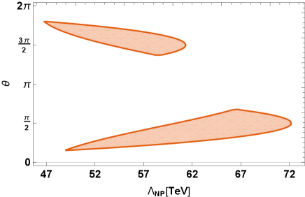
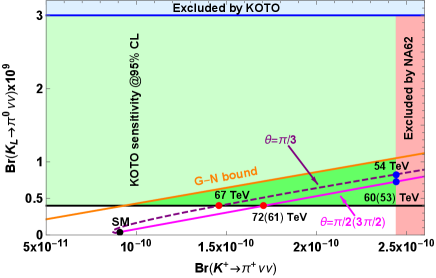
If we denote the Wilson coefficient as

Cdν,dim-6V,sdττ(Λχ)=Cdν,dim-6V,sdττ(ΛEW)eiθΛNP2,\displaystyle C_{d\nu,\text{dim-6}}^{V,sd\tau\tau}(\Lambda_{\chi})=C_{d\nu,\text{dim-6}}^{V,sd\tau\tau}(\Lambda_{\text{EW}})\equiv{e^{i\theta}\over\Lambda_{\rm NP}^{2}}, (75)

where θ\theta denotes the phase of the Wilson coefficient. Note that the running from the electroweak scale ΛEW\Lambda_{\text{EW}} to the chiral symmetry breaking scale Λχ\Lambda_{\chi} vanishes, as the dim-6 vector operators are not renormalized at one-loop level due to QCD Ward identity. The allowed range in the plane of [ΛNP,θ][\Lambda_{\text{NP}},\theta] is given in the left panel of Fig. 1. From this plot, we can see that the phase θ\theta is nonzero and the NP scale is limited to

ΛNP[47TeV,72TeV].\displaystyle\Lambda_{\rm NP}\in[47~{}\text{TeV},~{}72~{}\text{TeV}]\;. (76)

For specific choices of θ=π/2\theta=\pi/2 or 3π/23\pi/2, the real part of Cdν,dim-6V,sdττC_{d\nu,\text{dim-6}}^{V,sd\tau\tau} vanishes and both branching ratios are only governed by (Im[Cdν1,SMV,sdττ]+Im[Cdν,dim-6V,sdττ])2\left({\rm Im}[C_{d\nu 1,\text{SM}}^{V,sd\tau\tau}]+{\rm Im}[C_{d\nu,\text{dim-6}}^{V,sd\tau\tau}]\right)^{2}. Thus, in the plane of two branching ratios shown in the right panel of Fig. 1, the correlation lines for these two choices coincide with each other. The NP scale resides in the range of ΛNP[60TeV,72TeV]\Lambda_{\rm NP}\in[60~{}\text{TeV},~{}72~{}\text{TeV}] for θ=π/2\theta=\pi/2 or ΛNP[53TeV,61TeV]\Lambda_{\rm NP}\in[53~{}\text{TeV},~{}61~{}\text{TeV}] for θ=3π/2\theta=3\pi/2. We also display the case of θ=π/3\theta=\pi/3 resulting in a different line in the plane of two branching ratios.

Refer to caption
Refer to caption
Figure 1: Left: The allowed region in the [ΛNP,θ][\Lambda_{\text{NP}},\theta] plane. Right: The correlation of two Kaon decay branching ratios and constraint on the NP scale for the LNC operators, with θ=π/2\theta=\pi/2 or 3π/23\pi/2 (pink solid line) and θ=π/3\theta=\pi/3 (purple dashed line). The blue (red) points represent the lower (upper) limits of the NP scale. The sensitive region from KOTO 2016-2018 is shown in light green, and the excluded region by NA62 is in salmon. The light blue region is excluded by KOTO 2015. The black point corresponds the SM prediction.

On the other hand, for the LFV case, a similar analysis can be carried out based on Eqs. (6869). The SM has no interference with LFV contribution in this case. After neglecting the above LFC contribution from NP and assuming the coefficient with only one set of lepton flavors is switched on at a time, a lower limit on the NP scale associated with the LFV Wilson coefficients can be obtained as

ΛNP=|Cdν,dim-6V,sdαβ|12>56.4(63.3)TeV,forαβ,\displaystyle\Lambda_{\rm{NP}}=\Big{|}C_{d\nu,\text{dim-6}}^{V,sd\alpha\beta}\Big{|}^{-{1\over 2}}>56.4\ (63.3)~{}{\rm TeV},~{}\text{for}~{}\alpha\neq\beta\;, (77)

where the NA62 result for K+π+νν¯K^{+}\to\pi^{+}\nu\bar{\nu} at 95 (90)% CL is taken. A stronger bound can be set if we assume the same magnitude for all LFV Wilson coefficients, that is Cdν,dim6V,sdeμ=Cdν,dim6V,sdeτ=Cdν,dim6V,sdμτC_{d\nu,{\rm dim-6}}^{V,sde\mu}=C_{d\nu,{\rm dim-6}}^{V,sde\tau}=C_{d\nu,{\rm dim-6}}^{V,sd\mu\tau}

ΛNP>88(99)TeV,forαβ.\displaystyle\Lambda_{\rm{NP}}>88\ (99)~{}{\rm TeV},~{}\text{for}~{}\alpha\neq\beta\;. (78)

In Refs. Carpentier and Davidson (2010); He et al. (2019a, b), there are similar analyses for LFV coefficients using the limit on (K+π+νν¯){\mathcal{B}}(K^{+}\to\pi^{+}\nu\bar{\nu}) from PDG. Their limits can be translated into a bound on NP scale in our convention as 56.8 TeV in Ref. Carpentier and Davidson (2010) and 50 TeV in Refs. He et al. (2019a, b). We can see that the new NA62 result pushes the NP scale higher. The bound obtained above is the most stringent one for the coefficients with τ\tau flavor, compared to the bound from τ\tau lepton LFV rare decays He et al. (2019b). For the coefficients with (α,β)=(e,μ)(\alpha,\beta)=(e,\mu) or (μ,e)(\mu,e), the most stringent bound with ΛNP259TeV\Lambda_{\rm NP}\geq 259\,\mathrm{TeV} is from the charged lepton decay modes of Kaon, i.e. KLμe+,μ+eK_{L}\to\mu^{-}e^{+},\mu^{+}e^{-}. See also the derivation in Appendix B.

IV.2 Constraint on the LNV operator

In this section we assume the NP contribution from dim-6 LNC operators is negligible and therefore only keep the SM contribution in the LNC case. Under this assumption, we focus on the LNV NP contribution. As discussed above, the scalar LEFT operators from one dim-7 LNV operator in the SMEFT play an important role in the Kaon semi-invisible decays.

The Kaon invisible decays can entail constraint on the above Wilson coefficients. The effective Lagrangian for KLννK_{L}\to\nu\nu at the leading order is

KLνν\displaystyle\mathcal{L}_{K_{L}\to\nu\nu} =\displaystyle= iBF02[(Cdν1S,sdαβ+Cdν1S,dsαβCdν2S,sdαβCdν2S,dsαβ)(ναC¯νβ)\displaystyle{iBF_{0}\over 2}\Big{[}(C_{d\nu 1}^{S,sd\alpha\beta}+C_{d\nu 1}^{S,ds\alpha\beta}-C_{d\nu 2}^{S,sd\alpha\beta}-C_{d\nu 2}^{S,ds\alpha\beta})(\overline{\nu^{C}_{\alpha}}\nu_{\beta}) (79)
(Cdν1S,dsαβ+Cdν1S,sdαβCdν2S,dsαβCdν2S,sdαβ)(να¯νβC)]KL,\displaystyle-(C_{d\nu 1}^{S,ds\alpha\beta\ast}+C_{d\nu 1}^{S,sd\alpha\beta\ast}-C_{d\nu 2}^{S,ds\alpha\beta\ast}-C_{d\nu 2}^{S,sd\alpha\beta\ast})(\overline{\nu_{\alpha}}\nu^{C}_{\beta})\Big{]}K_{L}\;,

and that for KSννK_{S}\to\nu\nu decay is

KSνν\displaystyle\mathcal{L}_{K_{S}\to\nu\nu} =\displaystyle= iBF02[(Cdν1S,sdαβCdν1S,dsαβCdν2S,sdαβ+Cdν2S,dsαβ)(ναC¯νβ)\displaystyle{iBF_{0}\over 2}\Big{[}(C_{d\nu 1}^{S,sd\alpha\beta}-C_{d\nu 1}^{S,ds\alpha\beta}-C_{d\nu 2}^{S,sd\alpha\beta}+C_{d\nu 2}^{S,ds\alpha\beta})(\overline{\nu^{C}_{\alpha}}\nu_{\beta}) (80)
(Cdν1S,dsαβCdν1S,sdαβCdν2S,dsαβ+Cdν2S,sdαβ)(να¯νβC)]KS.\displaystyle-(C_{d\nu 1}^{S,ds\alpha\beta\ast}-C_{d\nu 1}^{S,sd\alpha\beta\ast}-C_{d\nu 2}^{S,ds\alpha\beta\ast}+C_{d\nu 2}^{S,sd\alpha\beta\ast})(\overline{\nu_{\alpha}}\nu^{C}_{\beta})\Big{]}K_{S}\;.

One can see that the processes are only induced by |ΔL|=2|\Delta L|=2 dim-6 operators in LEFT since they flip the helicity of one of neutrinos to allow the pseudoscalar Kaon to decay invisibly. The |ΔL|=0|\Delta L|=0 dim-6 operators 𝒪dν1/2V{\mathcal{O}}^{V}_{d\nu 1/2} are severely suppressed by the neutrino mass because they are subject to helicity-suppression. As seen in the above subsection, only the 𝒪dν1S{\mathcal{O}}^{S}_{d\nu 1} operator is induced by one dim-7 SMEFT operator at tree-level. By including the one-loop QCD running result for Cdν1SC_{d\nu 1}^{S} from electroweak scale ΛEWmW\Lambda_{\text{EW}}\approx m_{W} to the chiral symmetry breaking scale Λχ2GeV\Lambda_{\chi}\approx 2~{}{\rm GeV}, we obtain

Cdν1S(Λχ)=1.656Cdν1S(ΛEW).\displaystyle C_{d\nu 1}^{S}(\Lambda_{\chi})=1.656\ C_{d\nu 1}^{S}(\Lambda_{\text{EW}}). (81)

We further assume the Wilson coefficients in Eqs. (62-63) at ΛEW\Lambda_{\text{EW}} scale as

Cd¯LQLH11α2β(ΛEW)=Cd¯LQLH11β2α(ΛEW)=Cd¯LQLH12α1β(ΛEW)=Cd¯LQLH12β1α(ΛEW)1ΛNP3δαβ,\displaystyle C_{\bar{d}LQLH1}^{1\alpha 2\beta}(\Lambda_{\text{EW}})=C_{\bar{d}LQLH1}^{1\beta 2\alpha}(\Lambda_{\text{EW}})=C_{\bar{d}LQLH1}^{2\alpha 1\beta}(\Lambda_{\text{EW}})=C_{\bar{d}LQLH1}^{2\beta 1\alpha}(\Lambda_{\text{EW}})\equiv{1\over\Lambda_{\rm NP}^{3}}\delta_{\alpha\beta}, (82)

where ΛNP\Lambda_{\rm NP} denotes the NP scale above the electroweak scale. Combining Eqs. (79-80), the matching results in Eqs. (62-63), and the naive assumption in Eq. (82), we find that there is no tree-level contribution to KSK_{S} decay. For KLK_{L} invisible decay, we obtain the branching ratio of invisible decay

KLνν=2×3×12×mKLΓKLExp116π|0.585BF0vΛNP3|2,\displaystyle\mathcal{B}_{K_{L}\rightarrow\nu\nu}=2\times 3\times{1\over 2}\times{m_{K_{L}}\over\Gamma_{K_{L}}^{\text{Exp}}}{1\over 16\pi}\left|0.585{BF_{0}v\over\Lambda_{\rm NP}^{3}}\right|^{2}\;, (83)

where the factor 2 accounts for the anti-neutrino case, the factor 3 for the 3 generations of neutrinos, the factor 1/21/2 for the identical neutrinos in final states, and 1/16π1/16\pi for the phase space, respectively. The experimental bounds for the Kaon invisible decay were estimated in Ref. Gninenko (2015) as

KLinvisible\displaystyle\mathcal{B}_{K_{L}\rightarrow invisible} <\displaystyle< 6.3×10⁴(95%C.L.),\displaystyle 6.3\times 10^{-4}\ (95\%~{}\text{C.L.}), (84)
KSinvisible\displaystyle\mathcal{B}_{K_{S}\rightarrow invisible} <\displaystyle< 1.1×10⁴(95%C.L.).\displaystyle 1.1\times 10^{-4}\ (95\%~{}\text{C.L.}). (85)

The above KLK_{L} bound translates into a rather weak lower limit on the new physics scale

ΛNP4TeV.\displaystyle\Lambda_{\rm NP}\gtrsim 4\ {\rm TeV}\;. (86)

Given the matching results in Eqs. (62) and (63) together with the assumption in Eq. (82), the branching ratios of Kπνν^K\to\pi\nu\widehat{\nu} in Eqs. (31) and (32) can be simplified as

KLπ0νν^\displaystyle\mathcal{B}_{K_{L}\rightarrow\pi^{0}\nu\widehat{\nu}} =\displaystyle= J1KLαβ(112δαβ)|Cdν1S,dsαβ+Cdν1S,sdαβ|2+KLπ0νν¯SM\displaystyle J_{1}^{K_{L}}\sum_{\alpha\leq\beta}\left(1-{1\over 2}\delta_{\alpha\beta}\right)\left|C_{d\nu 1}^{S,ds\alpha\beta}+C_{d\nu 1}^{S,sd\alpha\beta}\right|^{2}+\mathcal{B}_{K_{L}\rightarrow\pi^{0}\nu\bar{\nu}}^{\text{SM}} (87)
=\displaystyle= 58.58GF3ΛNP6+KLπ0νν¯SM,\displaystyle{58.58\over G_{F}^{3}\Lambda^{6}_{\rm NP}}+\mathcal{B}_{K_{L}\rightarrow\pi^{0}\nu\bar{\nu}}^{\text{SM}}\;,
K+π+νν^\displaystyle\mathcal{B}_{K^{+}\rightarrow\pi^{+}\nu\widehat{\nu}} =\displaystyle= J1K+αβ(112δαβ)(|Cdν1S,dsαβ|2+|Cdν1S,sdαβ|2)+K+π+νν¯SM\displaystyle J_{1}^{K^{+}}\sum_{\alpha\leq\beta}\left(1-{1\over 2}\delta_{\alpha\beta}\right)\left(\left|C_{d\nu 1}^{S,ds\alpha\beta}\right|^{2}+\left|C_{d\nu 1}^{S,sd\alpha\beta}\right|^{2}\right)+\mathcal{B}_{K^{+}\rightarrow\pi^{+}\nu\bar{\nu}}^{\text{SM}} (88)
=\displaystyle= 13GF3ΛNP6+K+π+νν¯SM.\displaystyle{13\over G_{F}^{3}\Lambda^{6}_{\rm NP}}+\mathcal{B}_{K^{+}\rightarrow\pi^{+}\nu\bar{\nu}}^{\text{SM}}\;.
Refer to caption
Figure 2: The correlation of two Kaon decay branching ratios and constraint on the NP scale for the LNV operator. The labels and colors are the same as those in Fig. 1.

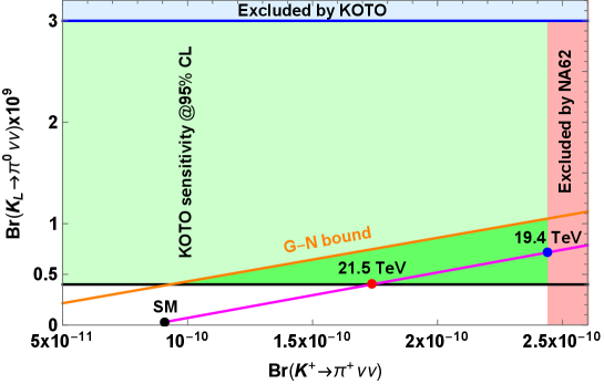
There is obviously no interference between the SM contribution and the LNV contribution. If we require those results to satisfy the region allowed by the KOTO and NA62 upper bounds, the NP contribution resides along the pink line in Fig. 2 and the NP scale is highly constrained to a narrow range

ΛNP[19.4TeV,21.5TeV].\displaystyle\Lambda_{\rm NP}\in[19.4~{}{\rm TeV},~{}21.5~{}{\rm TeV}]\;. (89)

See Fig. 2 for a more detailed illustration. This is an appealing scale both for LHC experiments and TeV scale seesaw mechanism yielding Majorana neutrino mass. This interpretation highly depends on the precision of the measurements and the simple assumption in Eq. (82). If we take the upper bound on K+π+νν¯\mathcal{B}_{K^{+}\rightarrow\pi^{+}\nu\bar{\nu}} from the NA62 experiment at 90% CL, that is K+π+νν^<1.85×10¹⁰\mathcal{B}_{K^{+}\rightarrow\pi^{+}\nu\widehat{\nu}}<1.85\times 10^{-10} Ruggiero , the contribution of the LNV operator together with the assumed Wilson coefficients in Eq. (82) is almost excluded. The analysis of the 2018 NA62 data would indicate if LNV operator can precipitate the discrepancy under the assumption.

The operator in Eq. (61) can also contribute to neutrinoless double beta (0νββ0\nu\beta\beta) decay. The NP scale from this process is constrained to be larger than 𝒪(100TeV){\mathcal{O}}(100~{}{\rm TeV}) Cirigliano et al. (2017); Liao and Ma (2019). Constraints from KπννK\to\pi\nu\nu are complementary and provide a similar sensitivity, because they constrain the quark flavor violating Wilson coefficients with an ss- and a dd-quark and any arbitrary generations of the lepton fields in the operator after relaxing the assumption in Eq. (82).

V Discussions and Conclusions

In the above analysis, we focus on the contact interactions from effective operators composed of s,ds,d quarks and two neutrinos for sdνν^s\to d\nu\widehat{\nu} transition, that is the so-called short-distance (SD) contribution. In addition, there exist the long-distance (LD) contributions to Kπνν¯K\to\pi\nu\bar{\nu} from the heavy NP parameterized by the dim-6 LNC operators in SMEFT. The LD contributions are mediated by light charged leptons, neutrinos or light meson propagators in the χ\chiPT picture. In the Kπνν¯K\to\pi\nu\bar{\nu} processes, it turns out that the LD contributions are negligible compared to the SD contribution and can be safely ignored. The detailed analysis is included in Appendix C.

In summary, we investigate the implication of Kπνν¯K\to\pi\nu\bar{\nu} from the recent KOTO and NA62 measurements for generic neutrino interactions in effective field theories. The interactions between quarks and left-handed SM neutrinos are first described by the LEFT below electroweak scale. We match them to χ\chiPT at the chiral symmetry breaking scale to calculate the branching fractions of Kaon semi-invisible decays and match them up to the SMEFT to constrain new physics above the electroweak scale.

In the framework of effective field theories, we prove that the Grossman-Nir bound is valid for both dim-6 and dim-7 LEFT operators in χ\chiPT, and the dim-6 scalar and vector operators dominantly contribute to the Kπνν^K\to\pi\nu\widehat{\nu} transition. They are induced by multiple dim-6 LNC operators and one dim-7 LNV operator in the SMEFT, respectively. After providing a generic constraint on the relevant Wilson coefficients, we separately discuss the constraints on the two kinds of operators. The LNC vector operators lead to interference with the SM contribution. We consider the lepton-flavor-conserving case and evaluate the constraints from Kaon leptonic decay modes KLe+e,μ+μK_{L}\to e^{+}e^{-},\mu^{+}\mu^{-}. For the ττ\tau\tau component in the sds\to d transition, the Kπνν¯K\to\pi\nu\bar{\nu} decays provide the only sensitive probe. We find the NP scale associated with the ττ\tau\tau Wilson coefficient is limited to be ΛNP[47TeV,72TeV]\Lambda_{\rm NP}\in[47~{}\text{TeV},~{}72~{}\text{TeV}].

One the other hand, we assume the NP contribution from dim-6 LNC operators is negligible and therefore only keep the SM prediction in the LNC case. As a result, the scalar LEFT operators from one dim-7 LNV operator in the SMEFT dominates the Kπνν^K\to\pi\nu\widehat{\nu} decay. We find that the KLK_{L} invisible decay KLννK_{L}\to\nu\nu places a weak bound on the new physics scale for the LNV operator. As there is no interference with the SM contribution, the constraint on the NP scale from Kπνν¯K\to\pi\nu\bar{\nu} is rather precise and resides in a narrow range ΛNP[19.4TeV,21.5TeV]\Lambda_{\rm NP}\in[19.4~{}{\rm TeV},~{}21.5~{}{\rm TeV}].

Appendix A The amplitudes and partial widths of Kπνν^K\to\pi\nu\widehat{\nu}

In this appendix we present details of the calculation of Kπνν^K\to\pi\nu\widehat{\nu}. For the process of K(pK)π(pπ)+να¯(p1)ν¯β(p2)/να(p1)νβ(p2)/να(p1)ν¯β(p2)K(p_{K})\to\pi(p_{\pi})+\overline{\nu_{\alpha}}(p_{1}){\overline{\nu}_{\beta}}(p_{2})/\nu_{\alpha}(p_{1})\nu_{\beta}(p_{2})/\nu_{\alpha}(p_{1}){\overline{\nu}_{\beta}}(p_{2}), the amplitudes for KLK_{L} decay are

iM1ΔL=2(KL)\displaystyle iM_{1}^{\Delta L=-2}(K_{L}) =\displaystyle= iB42(Cdν1S,sdαβ+Cdν2S,sdαβ+Cdν1S,dsαβ+Cdν2S,dsαβ)νT(p1)Cν(p2),\displaystyle{iB\over 4}2\left(C_{d\nu 1}^{S,sd\alpha\beta}+C_{d\nu 2}^{S,sd\alpha\beta}+C_{d\nu 1}^{S,ds\alpha\beta}+C_{d\nu 2}^{S,ds\alpha\beta}\right)\nu^{T}(p_{1})C\nu(p_{2})\;,
iM1ΔL=2(KL)\displaystyle iM_{1}^{\Delta L=2}(K_{L}) =\displaystyle= iB42(Cdν1S,dsαβ+Cdν2S,dsαβ+Cdν1S,sdαβ+Cdν2S,sdαβ)ν¯(p1)CνT¯(p2),\displaystyle{iB\over 4}2\left(C_{d\nu 1}^{S,ds\alpha\beta*}+C_{d\nu 2}^{S,ds\alpha\beta*}+C_{d\nu 1}^{S,sd\alpha\beta*}+C_{d\nu 2}^{S,sd\alpha\beta*}\right)\overline{\nu}(p_{1})C\overline{\nu^{T}}(p_{2})\;,
iM2ΔL=0(KL)\displaystyle iM_{2}^{\Delta L=0}(K_{L}) =\displaystyle= i4(Cdν1V,sdαβ+Cdν2V,sdαβCdν1V,dsαβCdν2V,dsαβ)(pK+pπ)μν¯(p1)γμν(p2),\displaystyle{i\over 4}\left(C_{d\nu 1}^{V,sd\alpha\beta}+C_{d\nu 2}^{V,sd\alpha\beta}-C_{d\nu 1}^{V,ds\alpha\beta}-C_{d\nu 2}^{V,ds\alpha\beta}\right)(p_{K}+p_{\pi})_{\mu}\overline{\nu}(p_{1})\gamma^{\mu}\nu(p_{2})\;, (90)

and those for K+K^{+} decay are

iM1ΔL=2(K+)\displaystyle iM_{1}^{\Delta L=-2}(K^{+}) =\displaystyle= iB22(Cdν1S,sdαβ+Cdν2S,sdαβ)νT(p1)Cν(p2),\displaystyle{-iB\over 2}2\left(C_{d\nu 1}^{S,sd\alpha\beta}+C_{d\nu 2}^{S,sd\alpha\beta}\right)\nu^{T}(p_{1})C\nu(p_{2})\;,
iM1ΔL=2(K+)\displaystyle iM_{1}^{\Delta L=2}(K^{+}) =\displaystyle= iB22(Cdν1S,dsαβ+Cdν2S,dsαβ)ν¯(p1)CνT¯(p2),\displaystyle{-iB\over 2}2\left(C_{d\nu 1}^{S,ds\alpha\beta*}+C_{d\nu 2}^{S,ds\alpha\beta*}\right)\overline{\nu}(p_{1})C\overline{\nu^{T}}(p_{2})\;,
iM2ΔL=0(K+)\displaystyle iM_{2}^{\Delta L=0}(K^{+}) =\displaystyle= i2(Cdν1V,sdαβ+Cdν2V,sdαβ)(pK+pπ)μν¯(p1)γμν(p2),\displaystyle{-i\over 2}\left(C_{d\nu 1}^{V,sd\alpha\beta}+C_{d\nu 2}^{V,sd\alpha\beta}\right)(p_{K}+p_{\pi})_{\mu}\overline{\nu}(p_{1})\gamma^{\mu}\nu(p_{2})\;, (91)

with α,β=e,μ,τ\alpha,\beta=e,\mu,\tau. The factor of 22 comes from the symmetry property of the operators and the corresponding Wilson coefficients for |ΔL|=2|\Delta L|=2. We neglect the masses of final state neutrinos and thus the different amplitudes do not interfere. After summing over all possible flavors, the flavor- and spin- summed squared matrix elements read

all|M(KL)|2\displaystyle\sum_{all}|M(K_{L})|^{2} =\displaystyle= αβspin(|M1ΔL=2(KL)|2+|M1ΔL=2(KL)|2)+α,βspin|M2ΔL=0(KL)|2\displaystyle\sum_{\alpha\leq\beta}\sum_{\rm spin}\left(|M_{1}^{\Delta L=-2}(K_{L})|^{2}+|M_{1}^{\Delta L=2}(K_{L})|^{2}\right)+\sum_{\alpha,\beta}\sum_{\rm spin}|M_{2}^{\Delta L=0}(K_{L})|^{2}
=\displaystyle= 2αβ(112δαβ)B24|Cdν1S,sdαβ+Cdν2S,sdαβ+Cdν1S,dsαβ+Cdν2S,dsαβ|2s\displaystyle 2\sum_{\alpha\leq\beta}\left(1-{1\over 2}\delta_{\alpha\beta}\right)\frac{B^{2}}{4}\left|C_{d\nu 1}^{S,sd\alpha\beta}+C_{d\nu 2}^{S,sd\alpha\beta}+C_{d\nu 1}^{S,ds\alpha\beta}+C_{d\nu 2}^{S,ds\alpha\beta}\right|^{2}s
+\displaystyle+ 14α,β|Cdν1V,sdαβ+Cdν2V,sdαβCdν1V,dsαβCdν2V,dsαβ|2((mK2t)(tmπ2)st)\displaystyle\frac{1}{4}\sum_{\alpha,\beta}\left|C_{d\nu 1}^{V,sd\alpha\beta}+C_{d\nu 2}^{V,sd\alpha\beta}-C_{d\nu 1}^{V,ds\alpha\beta}-C_{d\nu 2}^{V,ds\alpha\beta}\right|^{2}\left((m_{K}^{2}-t)(t-m_{\pi}^{2})-st\right)
all|M(K+)|2\displaystyle\sum_{all}|M(K^{+})|^{2} =\displaystyle= αβspin(|M1ΔL=2(K+)|2+|M1ΔL=2(K+)|2)+α,βspin|M2ΔL=0(K+)|2\displaystyle\sum_{\alpha\leq\beta}\sum_{\rm spin}\left(|M_{1}^{\Delta L=-2}(K^{+})|^{2}+|M_{1}^{\Delta L=2}(K^{+})|^{2}\right)+\sum_{\alpha,\beta}\sum_{\rm spin}|M_{2}^{\Delta L=0}(K^{+})|^{2} (93)
=\displaystyle= αβ(112δαβ)B2(|Cdν1S,sdαβ+Cdν2S,sdαβ|2+|Cdν1S,dsαβ+Cdν2S,dsαβ|2)s\displaystyle\sum_{\alpha\leq\beta}\left(1-{1\over 2}\delta_{\alpha\beta}\right)B^{2}\left(\left|C_{d\nu 1}^{S,sd\alpha\beta}+C_{d\nu 2}^{S,sd\alpha\beta}\right|^{2}+\left|C_{d\nu 1}^{S,ds\alpha\beta}+C_{d\nu 2}^{S,ds\alpha\beta}\right|^{2}\right)s
+\displaystyle+ α,β|Cdν1V,sdαβ+Cdν2V,sdαβ|2((mK2t)(tmπ2)st),\displaystyle\sum_{\alpha,\beta}\left|C_{d\nu 1}^{V,sd\alpha\beta}+C_{d\nu 2}^{V,sd\alpha\beta}\right|^{2}\left((m_{K}^{2}-t)(t-m_{\pi}^{2})-st\right),

where s=(p1+p2)2s=(p_{1}+p_{2})^{2} and t=(p2+pπ)2t=(p_{2}+p_{\pi})^{2}. Here αβ\alpha\leq\beta means that for |ΔL|=2|\Delta L|=2 we take αβ=ee,eμ,eτ,μμ,μτ,ττ\alpha\beta=ee,e\mu,e\tau,\mu\mu,\mu\tau,\tau\tau flavor configurations. One should note that the flavor indices α,β\alpha,\beta are implicitly summed over in the Lagrangian, while in the above amplitudes they denote the specific neutrino flavors in final states. The overall factor 2 in the second line for KLK_{L} decay is because the contributions from M1ΔL=2(KL)M_{1}^{\Delta L=2}(K_{L}) and M1ΔL=2(KL)M_{1}^{\Delta L=-2}(K_{L}) are the same for any pair of (α,β)(\alpha,\beta). The 1/2δαβ-1/2\delta_{\alpha\beta} accounts for the double counting of final state phase space for identical particles.

The partial decay width can be expressed as

ΓKπνν^=12mK1128π3mK20(mKmπ)2𝑑s𝑑t|(Kπνν)|2,\displaystyle\Gamma_{K\rightarrow\pi\nu\widehat{\nu}}=\frac{1}{2m_{K}}\frac{1}{128\pi^{3}m_{K}^{2}}\int_{0}^{(m_{K}-m_{\pi})^{2}}ds\int dt|\mathcal{M}(K\rightarrow\pi\nu\nu)|^{2}\;, (94)

where the integration interval of tt is

t[(E2+E3)2(E2+E32mπ2)2,(E2+E3)2(E2E32mπ2)2],\displaystyle t\in\left[\left(E_{2}^{*}+E_{3}^{*}\right)^{2}-\left(E_{2}^{*}+\sqrt{E_{3}^{*2}-m_{\pi}^{2}}\right)^{2},~{}\left(E_{2}^{*}+E_{3}^{*}\right)^{2}-\left(E_{2}^{*}-\sqrt{E_{3}^{*2}-m_{\pi}^{2}}\right)^{2}\right], (95)

with

E2=12s,E3=12mK2mπ2ss.\displaystyle E_{2}^{*}=\frac{1}{2}\sqrt{s},~{}E_{3}^{*}=\frac{1}{2}\frac{m_{K}^{2}-m_{\pi}^{2}-s}{\sqrt{s}}\;. (96)

The partial widths of Kaon semi-invisible decays are obtained by performing the tt integral

dΓKLπ0νν^ds\displaystyle{d\Gamma_{K_{L}\rightarrow\pi^{0}\nu\widehat{\nu}}\over ds} =\displaystyle= B229π3mK3αβ(112δαβ)|Cdν1S,sdαβ+Cdν2S,sdαβ+Cdν1S,dsαβ+Cdν2S,dsαβ|2\displaystyle{B^{2}\over 2^{9}\pi^{3}m_{K}^{3}}\sum_{\alpha\leq\beta}\left(1-{1\over 2}\delta_{\alpha\beta}\right)\left|C_{d\nu 1}^{S,sd\alpha\beta}+C_{d\nu 2}^{S,sd\alpha\beta}+C_{d\nu 1}^{S,ds\alpha\beta}+C_{d\nu 2}^{S,ds\alpha\beta}\right|^{2} (97)
×s((mK2+mπ2s)24mK2mπ2)1/2\displaystyle\times s\left((m_{K}^{2}+m_{\pi}^{2}-s)^{2}-4m_{K}^{2}m_{\pi}^{2}\right)^{1/2}
+13211π3mK3α,β|Cdν1V,sdαβ+Cdν2V,sdαβCdν1V,dsαβCdν2V,dsαβ|2\displaystyle+{1\over 3\cdot 2^{11}\pi^{3}m_{K}^{3}}\sum_{\alpha,\beta}\left|C_{d\nu 1}^{V,sd\alpha\beta}+C_{d\nu 2}^{V,sd\alpha\beta}-C_{d\nu 1}^{V,ds\alpha\beta}-C_{d\nu 2}^{V,ds\alpha\beta}\right|^{2}
×((mK2+mπ2s)24mK2mπ2)3/2,\displaystyle\times\left((m_{K}^{2}+m_{\pi}^{2}-s)^{2}-4m_{K}^{2}m_{\pi}^{2}\right)^{3/2},
dΓK+π+νν^ds\displaystyle{d\Gamma_{K^{+}\rightarrow\pi^{+}\nu\widehat{\nu}}\over ds} =\displaystyle= B228π3mK3αβ(112δαβ)(|Cdν1S,sdαβ+Cdν2S,sdαβ|2+|Cdν1S,dsαβ+Cdν2S,dsαβ|2)\displaystyle{B^{2}\over 2^{8}\pi^{3}m_{K}^{3}}\sum_{\alpha\leq\beta}\left(1-{1\over 2}\delta_{\alpha\beta}\right)\left(\left|C_{d\nu 1}^{S,sd\alpha\beta}+C_{d\nu 2}^{S,sd\alpha\beta}\right|^{2}+\left|C_{d\nu 1}^{S,ds\alpha\beta}+C_{d\nu 2}^{S,ds\alpha\beta}\right|^{2}\right) (98)
×s((mK2+mπ2s)24mK2mπ2)1/2\displaystyle\times s\left((m_{K}^{2}+m_{\pi}^{2}-s)^{2}-4m_{K}^{2}m_{\pi}^{2}\right)^{1/2}
+1329π3mK3α,β|Cdν1V,sdαβ+Cdν2V,sdαβ|2((mK2+mπ2s)24mK2mπ2)3/2.\displaystyle+{1\over 3\cdot 2^{9}\pi^{3}m_{K}^{3}}\sum_{\alpha,\beta}\left|C_{d\nu 1}^{V,sd\alpha\beta}+C_{d\nu 2}^{V,sd\alpha\beta}\right|^{2}\left((m_{K}^{2}+m_{\pi}^{2}-s)^{2}-4m_{K}^{2}m_{\pi}^{2}\right)^{3/2}.

Appendix B The constraints from leptonic Kaon decays

The current experimental constraints on the branching ratios of KSe+eK_{S}\to e^{+}e^{-} Ambrosino et al. (2009) and KSμ+μK_{S}\to\mu^{+}\mu^{-} Collaboration (2019) are

(KSe+e)\displaystyle{\mathcal{B}}(K_{S}\to e^{+}e^{-}) <9×10⁹,\displaystyle<9\times 10^{-9}\;, (KSμ+μ)\displaystyle{\mathcal{B}}(K_{S}\to\mu^{+}\mu^{-}) <2.4×10¹⁰,\displaystyle<2.4\times 10^{-10}\;, (99)

at 90% CL. The lepton-flavor-conserving modes of KLK_{L} decays have been measured Tanabashi et al. (2018)

(KLe+e)\displaystyle{\mathcal{B}}(K_{L}\to e^{+}e^{-}) =94+6×10¹²,\displaystyle=9^{+6}_{-4}\times 10^{-12}\;, (KLμ+μ)\displaystyle{\mathcal{B}}(K_{L}\to\mu^{+}\mu^{-}) =(6.84±0.11)×109.\displaystyle=(6.84\pm 0.11)\times 10^{-9}\;. (100)

Their SM predictions are Valencia (1998); Gomez Dumm and Pich (1998); D’Ambrosio and Kitahara (2017)

(KLe+e)SM\displaystyle{\mathcal{B}}(K_{L}\to e^{+}e^{-})_{\rm SM} 9×10¹²,\displaystyle\approx 9\times 10^{-12}\;, (KLμ+μ)SM\displaystyle{\mathcal{B}}(K_{L}\to\mu^{+}\mu^{-})_{\rm SM} =(6.85±0.86)×109.\displaystyle=(6.85\pm 0.86)\times 10^{-9}\;. (101)

We match the SMEFT Wilson coefficients in Eq. (59), relevant for Kaon physics, to the four vector operators in LEFT

𝒪de1V\displaystyle{\mathcal{O}}^{V}_{de1} =(dL¯γμdL)(eL¯γμeL),\displaystyle=(\overline{d_{L}}\gamma_{\mu}d_{L})(\overline{e_{L}}\gamma_{\mu}e_{L}), 𝒪de2V\displaystyle{\mathcal{O}}^{V}_{de2} =(dL¯γμdL)(eR¯γμeR),\displaystyle=(\overline{d_{L}}\gamma_{\mu}d_{L})(\overline{e_{R}}\gamma_{\mu}e_{R}), (102)
𝒪de3V\displaystyle{\mathcal{O}}^{V}_{de3} =(dR¯γμdR)(eL¯γμeL),\displaystyle=(\overline{d_{R}}\gamma_{\mu}d_{R})(\overline{e_{L}}\gamma_{\mu}e_{L}), 𝒪de4V\displaystyle{\mathcal{O}}^{V}_{de4} =(dR¯γμdR)(eR¯γμeR).\displaystyle=(\overline{d_{R}}\gamma_{\mu}d_{R})(\overline{e_{R}}\gamma_{\mu}e_{R}). (103)

The matching condition is given by222We do not include tensor operators 𝒪dW{\mathcal{O}}_{dW} and 𝒪dB{\mathcal{O}}_{dB} which are suppressed in χ\chiPT power counting relative to the vector-type operators, and also the scalar operators 𝒪dH{\mathcal{O}}_{dH} which are suppressed by the SM Yukawa couplings.

Cde1V,sdαβ\displaystyle C^{V,sd\alpha\beta}_{de1} =\displaystyle= DxsDyd(Clq(1),αβxy+Clq(3),αβxy(12sW2)(CHq(1),xy+CHq(3),xy)δαβ),\displaystyle D_{xs}^{*}D_{yd}\left(C_{lq}^{(1),\alpha\beta xy}+C_{lq}^{(3),\alpha\beta xy}-(1-2s_{W}^{2})\left(C_{Hq}^{(1),xy}+C_{Hq}^{(3),xy}\right)\delta_{\alpha\beta}\right), (104)
Cde2V,sdαβ\displaystyle C^{V,sd\alpha\beta}_{de2} =\displaystyle= DxsDyd2sW2(CHq(1),xy+CHq(3),xy)δαβ,\displaystyle D_{xs}^{*}D_{yd}2s_{W}^{2}\left(C_{Hq}^{(1),xy}+C_{Hq}^{(3),xy}\right)\delta_{\alpha\beta}, (105)
Cde3V,sdαβ\displaystyle C^{V,sd\alpha\beta}_{de3} =\displaystyle= Clqαβ21(12sW2)CHdsdδαβ,\displaystyle C_{lq}^{\alpha\beta 21}-(1-2s_{W}^{2})C_{Hd}^{sd}\delta_{\alpha\beta}, (106)
Cde4V,sdαβ\displaystyle C^{V,sd\alpha\beta}_{de4} =\displaystyle= 2sW2CHdsdδαβ.\displaystyle 2s_{W}^{2}C_{Hd}^{sd}\delta_{\alpha\beta}\;. (107)

The lepton-flavor-conserving decay widths are

(KX+)\displaystyle{\mathcal{B}}(K_{X}\to\ell^{+}\ell^{-}) =(KX+)SM+FK2m232πΓKXmKX24m2|CKX,dim-6V,sd|2+I.T.,\displaystyle={\mathcal{B}}(K_{X}\to\ell^{+}\ell^{-})_{\rm SM}+\frac{F_{K}^{2}m_{\ell}^{2}}{32\pi\Gamma_{K_{X}}}\sqrt{m_{K_{X}}^{2}-4m_{\ell}^{2}}\Big{|}C_{K_{X},\text{dim-6}}^{V,sd\ell\ell}\Big{|}^{2}+\framebox{I.T.}, (108)

where X=S,LX=S,L and FKF_{K} is the physical Kaon decay constant. I.T. stands for the interference term between the SM part and the NP part. Here the I.T. contribution is larger than the pure NP squared term in the above equation. To make a conservative estimation of the NP scale, we simply neglect the interference term below. Note that, once including the additional interference term, we should obtain a more stringent limit on the NP scale for eeee and μμ\mu\mu coefficients. The NP contribution is the linear combination of Wilson coefficients in Eqs. (104-107) and takes the form as

CKS,dim-6V,sd\displaystyle C_{K_{S},\text{dim-6}}^{V,sd\ell\ell} =(Cde1V,sdCde2V,sdCde3V,sd+Cde4V,sd)c.c.,\displaystyle=\left(C_{de1}^{V,sd\ell\ell}-C_{de2}^{V,sd\ell\ell}-C_{de3}^{V,sd\ell\ell}+C_{de4}^{V,sd\ell\ell}\right)-c.c.\;, (109)
CKL,dim-6V,sd\displaystyle C_{K_{L},\text{dim-6}}^{V,sd\ell\ell} =(Cde1V,sd+Cde2V,sd+Cde3V,sd+Cde4V,sd)+c.c..\displaystyle=\left(C_{de1}^{V,sd\ell\ell}+C_{de2}^{V,sd\ell\ell}+C_{de3}^{V,sd\ell\ell}+C_{de4}^{V,sd\ell\ell}\right)+c.c.\;. (110)

Considering the physical lifetime of KSK_{S} and KLK_{L} and the experimental constraints in Eqs. (99100), the stronger limit on NP scale is set by the KLK_{L} decays. After neglecting the interference term in Eq. (108) and subtracting the SM contribution in Eq. (101), the NP scales associated with the eeee and μμ\mu\mu coefficients are constrained to be

ΛNP=|CKL,dim-6V,sdμμ|1283TeV,\displaystyle\Lambda_{\rm NP}=\Big{|}C_{K_{L},\text{dim-6}}^{V,sd\mu\mu}\Big{|}^{-{1\over 2}}\geq 83~{}{\rm TeV}, (111)
ΛNP=|CKL,dim-6V,sdee|1220TeV.\displaystyle\Lambda_{\rm NP}=\Big{|}C_{K_{L},\text{dim-6}}^{V,sdee}\Big{|}^{-{1\over 2}}\geq 20~{}{\rm TeV}\;. (112)

Finally, we quote the result for the LFV mode KLμ±eK_{L}\to\mu^{\pm}e^{\mp}

(KLμ+e)=\displaystyle{\mathcal{B}}(K_{L}\to\mu^{+}e^{-})= (mKL2mμ2)2FK2m264πmKL3ΓKL|CKL,LFVV,sdeμ|2,\displaystyle\frac{(m_{K_{L}}^{2}-m_{\mu}^{2})^{2}F_{K}^{2}m_{\ell}^{2}}{64\pi m_{K_{L}}^{3}\Gamma_{K_{L}}}\Big{|}C_{K_{L},\rm LFV}^{V,sde\mu}\Big{|}^{2}\;, (113)
(KLμe+)=\displaystyle{\mathcal{B}}(K_{L}\to\mu^{-}e^{+})= (mKL2mμ2)2FK2m264πmKL3ΓKL|CKL,LFVV,sdμe|2,\displaystyle\frac{(m_{K_{L}}^{2}-m_{\mu}^{2})^{2}F_{K}^{2}m_{\ell}^{2}}{64\pi m_{K_{L}}^{3}\Gamma_{K_{L}}}\Big{|}C_{K_{L},\rm LFV}^{V,sd\mu e}\Big{|}^{2}\;, (114)
|CKL,LFVV,sd|2=|Cde2V,sdCde4V,sdc.c.|2+|Cde1V,sdCde3V,sdc.c.|2.\Big{|}C_{K_{L},\rm LFV}^{V,sd\ell\ell^{\prime}}\Big{|}^{2}=\Big{|}C_{de2}^{V,sd\ell\ell^{\prime}}-C_{de4}^{V,sd\ell\ell^{\prime}}-c.c.\Big{|}^{2}+\Big{|}C_{de1}^{V,sd\ell\ell^{\prime}}-C_{de3}^{V,sd\ell\ell^{\prime}}-c.c.\Big{|}^{2}\;. (115)

The upper limit on the lepton-flavor-violating decay of (KLe±μ)<0.47×10¹¹{\mathcal{B}}(K_{L}\to e^{\pm}\mu^{\mp})<0.47\times 10^{-11} at 90% CL Tanabashi et al. (2018) leads to a constraint on the NP scale of

ΛNP=|CKL,LFVV,sd|12 259TeV,\Lambda_{\rm NP}=\Big{|}C_{K_{L},\rm LFV}^{V,sd\ell\ell^{\prime}}\Big{|}^{-\tfrac{1}{2}}\geq\,259\ \mathrm{TeV}\;, (116)

with (,)=(e,μ)(\ell,\ell^{\prime})=(e,\mu) or (μ,e)(\mu,e).

Appendix C Long-distance contributions from dim-6 operators

Refer to caption
Figure 3: The topologies of LD contribution to Kπνν¯K\rightarrow\pi\nu\bar{\nu} in the context of χ\chiPT with the light charged leptons, neutrinos and Goldstone mesons as dynamical degrees of freedom. There also exist other topologies like the pure meson loops which we do not show here, since they are severely suppressed by additional loop factors and a χ\chiPT factor p/Λχp/\Lambda_{\chi} relative to the shown diagrams.

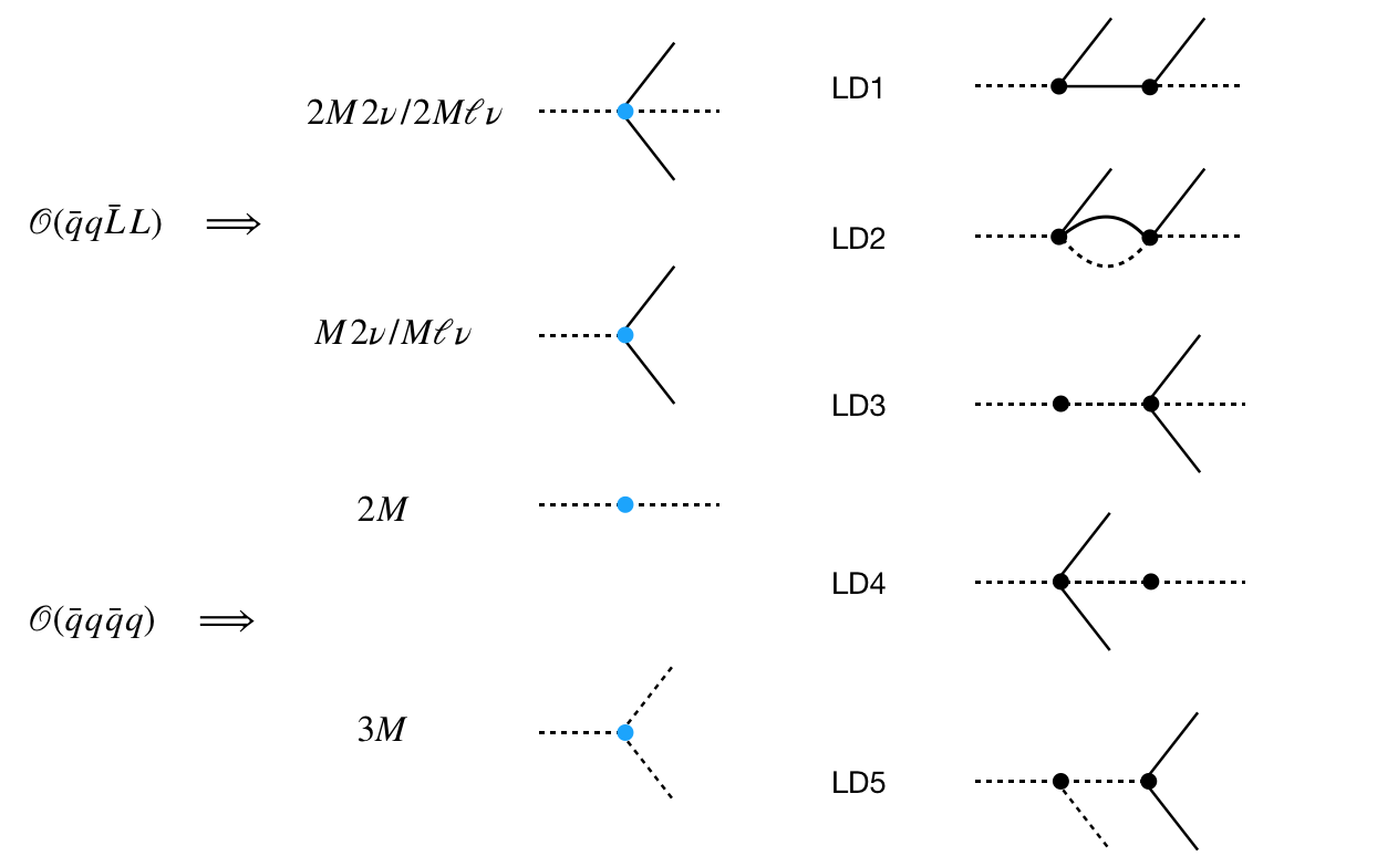
In this Appendix, we estimate the long distance (LD) contributions to Kπνν¯K\to\pi\nu\bar{\nu} from the heavy NP parameterized by the dim-6 LNC operators in SMEFT. The LD contributions are mediated by light charged leptons, neutrinos or light meson propagators in the χ\chiPT picture. In Fig. 3 we categorize the possible topologies for the LD contribution from the dim-6 two-quark-two-lepton operators 𝒪(q¯qL¯L){\mathcal{O}}(\bar{q}q\bar{L}L) and four-quark operators 𝒪(q¯qq¯q){\mathcal{O}}(\bar{q}q\bar{q}q) in SMEFT. The dashed and solid lines represent the possible meson and lepton fields, respectively.

The LD contributions mediated by neutrinos are suppressed compared to the SD contribution. In the Feynman diagrams for this kind of LD contribution, the vertex connecting the Kaon state involves the same Wilson coefficients as the SD case and the other vertex leads to one additional suppression factor GFG_{F}. Hence, we find that they are suppressed by F02GF107F_{0}^{2}G_{F}\sim 10^{-7}.

The LD contributions mediated by charged leptons can be induced by charged-current vector and/or scalar operators. The contribution from scalar operators is strongly constrained by charged pseudoscalar meson decays. The branching ratio for M+=K+,π+M^{+}=K^{+},\pi^{+} is

(M++ν)\displaystyle{\mathcal{B}}(M^{+}\to\ell^{+}\nu) i{m2|CduνV,αβi|2+B2|CduνS,αβi|2+I.T.,},\displaystyle\propto\sum_{i}\Big{\{}m_{\ell}^{2}\,\left|C_{du\nu\ell}^{V,\alpha\beta i\ell}\right|^{2}+B^{2}\,\left|C_{du\nu\ell}^{S,\alpha\beta i\ell}\right|^{2}+\framebox{I.T.},\Big{\}}\;, (117)

where we sum over neutrino flavor ii and CduνS,αβiCduν1S,αβiCduν2S,αβiC_{du\nu\ell}^{S,\alpha\beta i\ell}\equiv C_{du\nu\ell 1}^{S,\alpha\beta i\ell}-C_{du\nu\ell 2}^{S,\alpha\beta i\ell} (CduνV,αβiCduν1V,αβiCduν2V,αβiC_{du\nu\ell}^{V,\alpha\beta i\ell}\equiv C_{du\nu\ell 1}^{V,\alpha\beta i\ell}-C_{du\nu\ell 2}^{V,\alpha\beta i\ell}) denotes the scalar (vector) operator contribution. The SM contribution is helicity-suppressed and given by Cduν1V,αβi=22GFVαβC_{du\nu\ell 1}^{V,\alpha\beta i\ell}=2\sqrt{2}G_{F}V_{\alpha\beta}, while NP scalar contributions do not suffer from helicity-suppression. Requiring that the NP scalar contribution can be at most as large as the SM contribution translates into |CduνS,αβi|22GF|Vαβ|m/B|C_{du\nu\ell}^{S,\alpha\beta i\ell}|\lesssim 2\sqrt{2}G_{F}|V_{\alpha\beta}|m_{\ell}/B. The same scalar contribution enters the LD contribution to Kπνν¯K\to\pi\nu\bar{\nu} mediated by a charged lepton. After considering the phase space, the squared matrix element |K+π+νν¯ΔL=0|2=α,β|C^αβ|2((mK2t)(tmπ2)st)\left|\mathcal{M}_{K^{+}\rightarrow\pi^{+}\nu\bar{\nu}}^{\Delta L=0}\right|^{2}=\sum_{\alpha,\beta}|\hat{C}_{\alpha\beta}|^{2}\left((m_{K}^{2}-t)(t-m_{\pi}^{2})-st\right) is determined in terms of

|C^αβ|2\displaystyle|\hat{C}_{\alpha\beta}|^{2} =\displaystyle= |Cdν1V,sdαβ+Cdν2V,sdαβ|2+3×10³|B2CduνeS,suαμCduνeS,duμβ|2+I.T..\displaystyle\left|C_{d\nu 1}^{V,sd\alpha\beta}+C_{d\nu 2}^{V,sd\alpha\beta}\right|^{2}+3\times 10^{-3}\left|B^{2}C_{du\nu e}^{S,su\alpha\mu}C_{du\nu e}^{S,du\mu\beta*}\right|^{2}+\framebox{I.T.}\;. (118)

The second term is suppressed by a factor of 𝒪(105){\mathcal{O}}(10^{-5}) and consequently the LD scalar contribution is sub-dominant.

In the SM, the LD contribution induced by vector operators is suppressed by 𝒪(104){\mathcal{O}}(10^{-4}) relative to the SD contribution Hagelin and Littenberg (1989). As the NP contribution to charged current operators is at most of the same order as the SM contribution, the LD contribution from vector operators is negligible.

Similarly, the meson-mediated tree-level contributions (LD3 and LD4) are suppressed by 𝒪(104){\mathcal{O}}(10^{-4}) with respect to the SD contribution Hagelin and Littenberg (1989); Lu and Wise (1994) in the SM, while the one-loop contribution LD2 is of the same order as the LD1 contribution in the SM Rein and Sehgal (1989); Buchalla and Isidori (1998). To our knowledge, there is no general LEFT analysis of LD contributions to Kπνν¯K\to\pi\nu\bar{\nu}. As four quark operators with ΔS=1\Delta S=1 directly contribute to hadronic Kaon decays of which many have been measured at sub-percent level precision, we expect that similar conclusions hold for NP contributions mediated by meson exchange. In summary, currently it is safe to neglect long-distance contributions to Kπνν¯K\to\pi\nu\bar{\nu}.

Acknowledgements.
We would like to thank Xiao-Gang He, Yi Liao, Jusak Tandean and Jian Zhang for very useful discussions and communication. TL is supported by the National Natural Science Foundation of China (Grant No. 11975129) and “the Fundamental Research Funds for the Central Universities”, Nankai University (Grants No. 63191522, 63196013). XDM is supported by the MOST (Grant No. MOST 106-2112-M-002-003-MY3).

References