∎
22email: [email protected] 33institutetext: J. Rodriguez Rincon 44institutetext: Simon A. Levin Mathematical and Computational Modeling Sciences Center, Arizona State University, Tempe, AZ 85281, USA.
44email: [email protected] 55institutetext: G. DeGrandi-Hoffman 66institutetext: Carl Hayden Bee Research Center, United States Department of Agriculture-Agricultural Research Service, Tucson, AZ 85719, USA.
66email: [email protected] 77institutetext: J. Fewell 88institutetext: Life Sciences, Arizona State University, Tempe, AZ 85287, USA.
88email: [email protected] 99institutetext: J. Harrison 1010institutetext: Life Sciences, Arizona State University, Tempe, AZ 85287, USA.
1010email: [email protected] 1111institutetext: Y. Kang 1212institutetext: Sciences and Mathematics Faculty, College of Integrative Sciences and Arts, Arizona State University, Mesa, AZ 85212, USA
1212email: [email protected]
Impacts of seasonality and parasitism on honey bee population dynamics ††thanks:
Abstract
The honeybee plays an extremely important role in ecosystem stability and diversity and in the production of bee pollinated crops. Honey bees and other pollinators are under threat from the combined effects of nutritional stress, parasitism, pesticides, and climate change that impact the timing, duration, and variability of seasonal events. To understand how parasitism and seasonality influence honey bee colonies separately and interactively, we developed a non-autonomous nonlinear honeybee-parasite interaction differential equation model that incorporates seasonality into the egg-laying rate of the queen. Our theoretical results show that parasitism negatively impacts the honey bee population either by decreasing colony size or destabilizing population dynamics through supercritical or subcritical Hopf-bifurcations depending on conditions. Our bifurcation analysis and simulations suggest that seasonality alone may have positive or negative impacts on the survival of honey bee colonies. More specifically, our study indicates that (1) the timing of the maximum egg-laying rate seems to determine when seasonality has positive or negative impacts; and (2) when the period of seasonality is large it can lead to the colony collapsing. Our study further suggests that the synergistic influences of parasitism and seasonality can lead to complicated dynamics that may positively and negatively impact the honey bee colony’s survival. Our work partially uncovers the intrinsic effects of climate change and parasites, which potentially provide essential insights into how best to maintain or improve a honey bee colony’s health.
Keywords:
Honey Bees Seasonality Parasitism Climate Change1 Introduction
Honey bee, Apis mellifera, the colony is not only an excellent example of a complex adaptive system wilson2000sociobiology , but also has great value to our ecosystem and economic development. Per USDA statistics, 80% of crops benefit from pollination by honey bees, including more than 130 types of fruits and vegetables USDApollinate , worth $215 billion annually worldwide smith2013pathogens . Additionally, honey bees produce honey and other hive products that are beneficial to human health. For example, the average American consumed 1.0 pounds of honey per person in 2019, which has increased from 0.5 pounds in 1990 USDA . Unfortunately, honey bee colonies are collapsing at an alarming rate, especially during winter neumann2010micro causing unsustainable losses to commercial beekeepers and colony shortages to growers.
Research perry2015rapid ; oldroyd2007s ; smith2013pathogens suggests that there are many factors contributing to the global decline of the honey bee population. Those factors include nutritional stress from lack of flowering plants, environmental stressors such as global warming, lack of genetic variation, and vitality, parasites such as Varroa mites and Nosema, and diseases such as acute bee paralysis virus and deformed wing virus. Most notably, Varroa mites pose a huge threat to the health of honey bees Peng:1987aa ; Vetharaniam:2006aa ; degrandi2004mathematical ; messan2017migration ; messan2021population ; kang2016disease . They can parasitize honey bees, transmit viruses, and also make honey bees more susceptible to viral outbreaks koleoglu2017effect . Mites parasitize workers and drones (male bees), larvae and adults, but not the queen degrandi2017dispersal . Parasitized honey bees have shortened lifespans, lower weight, and weakened immune systems Peng:1987aa . Foragers that have been parasitized during development are more easily disoriented during foraging as adults koleoglu2017effect . Infected colonies also are more prone to viral diseases and struggle to survive in the winter degrandi2019economics ; degrandi2004mathematical ; martin2012global ; chen2007honey .
Seasonality has important effects on honey bee foraging behaviors. For example, in temperate areas during in fall and winter, food can become unavailable as temperatures drop below freezing. During this time, honey bees remain in their hives and form a thermoregulated cluster of bees stabentheiner2003endothermic , but if the bees fail to maintain cluster warmth, the colony will perish simpson1961nest . Moreover, the queen bee stops or reduces egg laying seeley1985survival ; degrandi1989beepop ; seasonality in preparation for overwintering martin2001role . Overwintering is stressful to colonies and losses may exceed 30% doeke2015overwintering .
Both experimental and simulated bee population data show seasonal patterns in colony population dynamics degrandi1989beepop ; harris1980population .
Seasonality also plays a role in the dynamics of parasites and viruses in colonies degrandi2004mathematical ; martin2001role ; smolinski2021raised . Thus, there is increased attention to including seasonality in honey bee population models. For example, ratti2015mathematical ; eberl2010importance ; sumpter2004dynamics adding seasonality equations using four sets of parameter values to differentiate seasons revealed that seasonal dynamics can lead to colonies with persistant Varroa infestations to suddenly collapse in late fall or spring because of the compounding effects of parasitism and viruses transmitted by Varroa ratti2015mathematical . The seasonal models also generated recommendations that controls for Varroa should occur in summer to reduce the colony losses sumpter2004dynamics . The work of betti2016age ; betti2014effects directly used two sets of models to represent the dynamics of non-winter and winter, respectively. The model betti2014effects has no egg laying in the winter system and considering the age structure of the colony during its yearly cycle. The model betti2016age added 21-day transition equations for colonies to wake-up between the end-of-winter and a new active season. This model captured the sharp decline in colony size often seen in the spring (spring dwindling) and showed that the timing of the onset of disease in a colony can impact its severity and persistence in the population.
Here, motivated by the experimental work shown in degrandi1989beepop ; harris1980population , we describe a model where seasonality has been incorporated into the queen’s egg-laying rate through cosine functions.
An age-structure model of honey bees’ population dynamics Chen et al. (2020) chen2020model showed that seasonality may reduce colony survival but may also prevent colony collapse. Messan et al. (2021) messan2021population focused on the colonies with parasites, and found seasonality can help colonies recover under certain conditions. Messan et al. (2018) messan2018effects focused on the nutrition of colonies, and found that seasonality can effects from stress and cause colony death.
Based on the data kang2016disease ; degrandi1989beepop and previously reported models chen2020model ; messan2018effects ; messan2021population , we formulate a mathematical modeling framework describing honeybee-mite interactions with seasonality in the queen’s egg-laying rate to address the following questions:
-
•
How may seasonality impact honey bee populations in the absence of parasitism?
-
•
How may parasitism impact the honey bee population?
-
•
What are the synergistic impacts of seasonality and parasitism on the honey bee population?
The remaining parts of this article are structured as follows: In Section 2, we provide details of how we modeled seasonality in the egg-laying rate and a general modeling framework for the interactions of parasitism and honey bees. In Section 3, we address how seasonality impacts the survival of honey bee colonies and their population dynamics. We theoretically demonstrate the impacts of parasitism on the honey bee populations without seasonality. In Section 4, we explore how parasites and seasonality might influence colony survival and population dynamics. In the last section, we conclude our theoretical and bifurcation analysis results regarding the effects of seasonality and parasites on colony dynamics and propose future studies needed for understanding how climate-related factors may threaten honey bee colonies.
2 Model Derivation
In this section, we focus on modeling the honeybee-parasite colony dynamics with seasonality. Let be the population of the honey bee and be the population of the mites in a given colony at time . We assume that:
-
A1:
The term reflects the cooperative brood care from adult bees that perform nursing and collecting food for brood chen2020model ; messan2021population ; messan2018effects ; schmickl2007hopomo ; kang2016disease ; eischen1984some , where indicates the colony size at which brood survival rate is half maximum.
-
A2:
We assume that the queen egg-laying rate is seasonal () due to resource constraints. The literature work suggests that food, temperature, weather, and oviposition place would affect the queen bodenheimer1937studies ; khoury2011quantitative ; degrandi1989beepop . Motivated by literature chen2020model ; messan2021population ; chen2021review and analysis of recent experimental data fisher2021colony , we model the egg-laying rate with seasonality as follows:
(1) with measuring the intensity of seasonal impacts, representing the average of egg-laying rate, representing the length of seasonality, and being the time of the maximum laying rate.
-
A3:
Female mites breed offspring in the cell, and complete the mating in the cell. In the phoretic phase, female mites feed on adult bees and immigrate to other colonies Vetharaniam:2006aa . In the reproductive phase, mites attach to foraging bees and then reproduce offspring in the cell ramsey2019varroa . Based on the biological background and literature work messan2021population ; betti2014effects ; sumpter2004dynamics , we model the honeybee-parasite interaction as follows:
where is the mite parasitism rate to the honey bee, is parasite attachment effects, and is the size of honey bee population at which rate of attachment is half maximal.
-
A4:
Female mites need nutrition from honey bees to produce the next generation. The parameter indicates conversion rate of nutrient consumption obtained from bees into nutrients needed by mites to reproduce.
The four assumptions above lead to the following nonautonomous and non-linear ordinary differential equations of the honeybee-parasite interaction model with seasonality (Model (2)):
| (2) |
with .
Note: If and , Model (2) reduces to the previous work of Kang et al. (2016) kang2016disease disease free model; and if , Model (2) reduces to our previous works of Messan et al. (2017 & 2021) messan2017migration ; messan2021population . Thus the current model (2) processes the general interaction properties of honey bees and parasitism.
| Parameter | Definition (Units) | Parameter | Definition (Units) | ||||||
| H | Honey bee population (bees) | M | Parasite (mites) population (bees) | ||||||
| a | The parasitism rate to honey bee (per day) | b |
|
||||||
| c | Parasite attachment effects | The average of egg-laying rate (bees/day) | |||||||
|
|
||||||||
| & |
|
the length of seasonality (days) | |||||||
|
the strength of seasonality |
In the following two sections, we will provide our detailed study to obtain insights regarding how may seasonality and/or parasitism alone or combined impact honey bee population dynamics.
3 Mathematics Analysis
To facilitate our analysis of the proposed system, we start with re-scaling our system (2). Assume that , and , let , , , , , and , then system (2) can scaled by following:
| (3) |
We first show that the proposed model (3) is positive invariant and bounded in as the following theorem:
Theorem 3.1
Assume that all parameters are non-negative. Model (3) with initial value , , and possesses a unique solution, and the space is positively invariant and bounded in .
Remark 1
3.1 Impact of Seasonality on Honeybee-Only Population Dynamics
If there is no mites, i.e., , the model (2) reduces to the following bee-only population model with seasonality:
| (4) |
with which satisfies a Lipschitz condition for all . Thus according to Theorem 3.1, the initial value problem with has a unique non-negative and bounded solution.
In order to study the effects of the strength of seasonality () and the length of seasonality () on bee populations, we start with the dynamics of the Honeybee-only model (4) when is a constant. The honeybee-only system without seasonality (4) has two equilibria shown as below provided :
The global dynamics of (4) when can be summaries as the following proposition:
Proposition 1
If , then the population of converges to 0 for any initial condition . In the case that , converges to 0 for any initial condition while converges to for any initial condition .
Notes: Proposition 1 indicates that the relationship among the constant egg-laying rate , the honey bee mortality, and the half-maximum rate , as well as initial conditions, determine whether the honey bee colony can survive. With the larger egg-laying rate with the larger initial condition , the honey bee colony is more likely to survive.
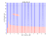
In the case that the egg-laying rate is seasonal, with its average value over each seasonal length being , the consequence of honey bee population dynamics can be complicated. Examples shown in Figure 1 suggest that the seasonality in the egg-laying rate can promote the survival of honey bees when the intensity of seasonality is not too high, and it can also make the honey bee colony prone to collapsing when the intensity of seasonality is high.
In Figure 1, without seasonality , the honey bee colony with , , , and can survive under its initial condition (red curve in Figure 1(a)) while it collapses under its initial condition (red curve in Figure 1(b)). When the intensity of seasonality is not too high, i.e., or , the honey bee colony can survive under its initial condition (black and green curves in Figure 1(b)). This is an example showing that seasonality can promote the survival of a honey bee colony. On the other hand, When the intensity of seasonality is high, i.e., (blue curve in Figure 1(a)), the honey bee colony collapses with the initial condition of when the honey bee colony can survive without seasonality. This is an example showing that seasonality can make honey bee colony collapse under certain conditions.


In order to explore the impact of the intensity of seasonality , we first define the minimum and maximum value of the egg-laying rate function: and . Motivated by Proposition 1, the intensity of seasonality can be classified into the following three cases:
-
1.
The low egg-laying rate if . This case is equivalent to
-
2.
The high egg-laying rate if . This case is equivalent to
-
3.
The intermediate egg-laying rate if . This is the case when
Now we have the following theorem:
Theorem 3.2
Let and . If the egg-laying rate is low, i.e., , the honey bee population converges to zero for any initial condition . In the case that the egg-laying rate is high, i.e., , honey bee population can survive if the initial condition . More specifically, we have
if and .
Notes: Theorem 3.2 implies that we can focus on how seasonality impacts honey bee population when the egg-laying rate is not low, i.e., which includes the case 2 and 3. Because the low egg-laying rate leads the colony to collapse. Thus, we can reduce the three cases above to the following two cases by introducing the critical intensity of seasonality
-
1.
The low intensity of seasonality, i.e.,
-
2.
The high intensity of seasonality, i.e.,
By applying Proposition 3.1 and the method used in Ratti et al.(2015) ratti2015mathematical , we obtain the stability condition when Model 4 processes a periodic solution as the following theorem:
Theorem 3.3
Suppose are periodic solutions of the Model 4, and . Then is stable if , or is unstable if , where .
Notes: Theorem 3.3 shows that the stability of the periodic solution of Model 4 requires , thus is always locally stable as the case without seasonality.


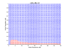
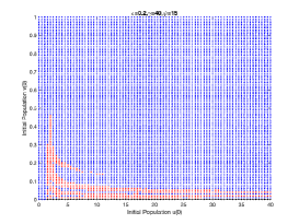
To further address the impacts of seasonality on honey bee population dynamics, we provide basins of attractions for Model (4) in Figure 2 and Figure 3 by setting .
We set in Figure 2. The x-axis is the initial honey bee population , and the y-axis is the intensity of seasonality measured by . Those parameter values gives which is a white horizontal line in Figure 2 and Figure 3.
The blue region in Figures is the value of the strength of seasonality () and the corresponding initial conditions that lead the colony to collapse, while the red region is the value of and that lead to the colony survival.
Figure 2 and Figure 3 suggest that the strength of seasonality (), the length of seasonality (), and the time of the maximum laying rate () impact the survival of honey bee colony in the synergistic ways:
-
1.
The length of seasonality () is small, e.g., :
-
•
If the time of the maximum laying rate () is less than the half period , the seasonality seems to promote the survival of the colony in the sense that the initial bee population that originally leads to collapsing but it leads to colony survival with seasonality.
-
•
If the time of the maximum laying rate () is larger than the half period , the seasonality seems to suppress the survival of the colony in the sense that the initial bee population that originally leads to survival but it leads to colony collapsing with seasonality.
-
•
-
2.
When the length of seasonality () is larger, e.g., , the large intensity of seasonality can lead to the collapsing of the colony while the impacts of the smaller intensity of seasonality depends on the timing of the maximum laying rate () as follows:
-
•
If the time of the maximum laying rate () is less than the half period , the seasonality seems to promote the survival of the colony.
-
•
If the time of the maximum laying rate () is larger than the half period , the seasonality seems to suppress the survival of the colony.
-
•
3.2 Impact of Parasitism on honey bee Population without Seasonality
In this subsection, we focus on dynamics of the honeybee-parasite interaction model (3) in the absence of seasonality, i.e., . Thus, we have the following rescaled model (5):
| (5) |
that would allow us to obtain biological insights on how parasitism impacts the honey bee population by comparing the dynamics of versus . In the case that , the model (3) reduces to the honey bee only model in the constant environment (4) whose dynamics are summarized in Proposition 1.
Let be an equilibrium of Model (3), then it satisfies the following equations:
| (6) |
| (7) |
Solving Eqt.7 gives or . And if , then Eqt.6 is
which gives the following two positive solutions provided that ,
or
In the case that , we have and as the unique interior equilibrium of Model 3. The stability of the equilibrium point can be evaluated through the following Jacobean matrix of Model 3 is
Now we are the following on the dynamics of the Honeybee-Parasite system (3):
Theorem 3.4
[Dynamics of Honeybee-Parasite system (3)] The system (3) can have one, three, or four equilibria whose existence and stability conditions are listed in Table 1. The global dynamics of Model (3) can be summarized as follows:
-
1.
The system (3) converges to extinction for almost all initial conditions if one the three conditions holds (1); (2) ; or (3).
-
2.
If or , depending on initial condition, the trajectory of system (3) converges to either or .
-
3.
If , then system (3) has a unique interior equilibrium which is locally asymptotically stable when and is a source when .
| Equilibria | Existence condition | Stability condition |
|---|---|---|
| Always exists | Always locally stable | |
| Saddle if ; Source if or | ||
| Sink if or ; Saddle if | ||
| & | Sink if ; Source if |
Notes: Theorem 3.4 provides us a global picture of the dynamics of the system (3) and the related biological implications of the impact of parasitism on honey bee population dynamics in constant conditions. Theorem 3.4 suggests that parasitism can have negative impacts on the honey bee population in three ways: (1) May lead to the collapsing of the colony; (2) May lead to the coexistence of both honey bee and parasitism but the honey bee population decreases compared to the case without parasitism, or (3) May destabilize the honey bee population.
Item (3) needs further theoretical exploration regarding how may parasitism destabilize the colony dynamics. For example, the colony destabilizes to show fluctuating dynamics through supercritical Hopf-bifurcation; or to collapse supercritical Hopf-bifurcation.
By applying the results in wang2011predator , our system 3 undergoes a Hopf-bifurcation. To study further, we re-scaled the system 3 to the following model:
| (8) |
where and . We can verify that our system 8 satisfies the following conditions:
(a1) , where ; is positive for , and is negative otherwise; there exists such that on , on ;
(a2) ; for and for , and there exists such that .
(a3) and are near and .
Then according to Theorem 3.1 in Wei et al. (2011) wang2011predator , we can conclude that our system 8 exists the first Lyapunov coefficient
where
| (9) |
Thus, we have the following results on Hopf-bifurcations:
Theorem 3.5
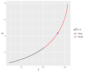
The system 3 undergoes a supercritical Hopf-bifurcation at with , and a subcritical Hopf-bifurcation at with .
Note: Theorem 3.5 implies that the system 3 can undergo a supercritical or subcritical Hopf-bifurcation depending on the relationship between and . If the system goes supercritical bifurcation at , then it has a stable limit cycle surrounding a source equilibrium when . When the system 3 undergoes a subcritical Hopf-bifurcation, then both population of honey bees and the parasitic mites go to zero through the unstable limit cycle. Biologically, it implies that parasitism in the constant environment can destabilize the dynamics and even lead to colony collapse, thus parasitism has negative impacts on honey bee population dynamics.
4 Synergistic Impacts of Parasitism and Seasonality
In the previous two sections, we explore the impacts of seasonality on the honey bee population and the impacts of parasitism on the honey bee population in a constant environment, respectively. Our study shows that seasonality can have positive or negative effects on the survival of honey bee colonies depending on the values of the strength of seasonality , the period , and the timing of the maximum egg-laying rate . Our theoretical work shows that parasitism in general has negative impacts on the survival of honey bee colonies in a constant environment.
In this section, we will explore how seasonality combined with parasitism affects honey bee population dynamics. We start with the following theorem regarding the stability condition when Model 3 processes a periodic solution of by applying Floquet theory theorem and the approach in Ratti et al.(2015) ratti2015mathematical .
Theorem 4.1
Note: Theorem 4.1 implies that is always locally stable, thus initial conditions play important roles in the survival of honeybee colonies.
By comparing the results of Theorem 3.4 and Theorem 4.1, we can see that the impact of seasonality: the seasonality in the egg laying rate generates the periodic solution whose stability requires . Those conditions reduce to and when being a constant.
By comparing the results of Theorem 3.3 and Theorem 4.1, we can see the impact of parasitism. Specifically, the stability of nontrial periodic boundary solution requires .
Note that our honeybee-parasite model (4) exhibits strong Allee effects in honey bees due to collaborative behavior in the colony. There is limited theoretical work on exploring the impacts of both parasitism and seasonality. Ratti et al.(2015)ratti2015mathematical developed a honeybee-mite-virus model with seasonality. Their model also exhibits strong Allee effects in honey bees while their mite-free solution is always unstable due to their formulation of the mite population. They discussed the existence of periodic solution and its stability in the bee-only model and discussed the stability of the disease-free solution and mite-free solution through linearization and the method of Floquet theory in the bee-mite model and bee-mite-virus model respectively. The most recent work that can be related to our topic is the paper by Rebelo and Soresina (2020) rebelo2020coexistence . Their paper proposed and studied a prey-predator model with weak or strong Allee effects in a periodic environment. They discussed the stability conditions of trivial, nontrivial solutions, and periodic solutions. They also showed that different initial conditions might lead to the extinction of both species or the coexistence of two species that converges to a stable periodic orbit.
To further our understanding of the impacts of seasonality and parasitism, we perform simple time series simulations and observe the following by setting
-
1.
In the absence of seasonality and parasitism, a honey bee colony can establish its population when its initial condition is greater than otherwise, it collapses.
- 2.
-
3.
With parasitism but without seasonality, a honey bee colony can survive through the stable limit cycle around the interior equilibrium for the right initial conditions. For example, a honey bee colony survives when and (see the red curve in Figure 5(a)) while it collapses when the initial parasites population grows up to (see the red curve in 5(b)).

(a) Seasonality promotes honey bee survival 
(b) Seasonality leads to the colony collapsing Figure 4: Comparison examples of seasonality having positive or negative effects in the honey bee colony survival without parasitism. Red curves are honey bee populations without seasonality and black curves are honey bee populations with seasonality. -
4.
With both seasonality and parasitism, Figure 5(b) suggests that seasonality can promote the survival of a honey bee colony when the parasite’s initial population is and the seasonality can also make the honey bee colony prone to collapse when the parasite initial population is (see Figure 5(a)).

(a) Seasonality promotes honey bee survival 
(b) Seasonality leads to the colony collapsing Figure 5: Comparison examples of seasonality having positive or negative effects in the honey bee colony survival with parasitism. Red curves are the honey bee populations without seasonality and black curves are the honey bee population with seasonality.
The observations above suggest that seasonality combined with parasitism may have positive or negative impacts on the honey bee colony survival depending on varied conditions. To explore further, we will perform a bifurcation analysis to understand how may the strength of seasonality , the length of seasonal period , the timing of the maximum egg-laying rate , and the severity of parasitism measured by in the following two scenarios of honeybee-parasitism dynamics in the absence of seasonality:
-
•
Honey bee and parasitism Coexists at a stable equilibrium
-
•
Honey bee and parasitism Coexists as a stable limit cycle
4.1 Impacts of seasonality on the stable equilibrium coexistence
We choose a typical example of our honeybee-parasite interaction model (3) by setting
which has a bistability between the colony collapsing state and the survival equilibrium at the locally stable equilibrium point whose basins of attractions are red area shown in Figure 6(a).
To further explore the impacts of the seasonality strength and the period of seasonality on the colony survival and population dynamics, without loss of generosity, we set the queen laying her maximum number of eggs at time , and we perform the following simulations (Figure 6, 7, 8) on basin’s attractions of our honeybee-parasite model (3).
-
1.
When the period of the seasonality is small, e.g., , comparisons of areas of basin attractions for the colony survival among Figure 6(a) (no seasonality), 6(c) (the seasonality strength ), and 6(d) (the seasonality strength ), suggest that seasonality strength may not impact the basin attractions of the colony survival but it impacts the population dynamics as shown in Figure 6(b). Simulations suggest that the larger value of the strength of seasonality , the larger amplitude of the population.

(a) no seasonality 
(b) Honey bee Population for those three cases 
(c) 
(d) Figure 6: Impacts of seasonality on the honey bee colony survival when the period of seasonality is large; and , , and and . Initial population is , and . The blue area is the basin attraction that leads to colony collapse, while the red area is the basin attraction the colony can survive. -
2.
When the period of the seasonality is in the intermediate range, e.g., , the impacts from the strength seasonality can be very complicated. For example, Figure 7(d) shows that basins of attractions for the colony survival are splitted into two red areas, and Figure 7(b) shows larger gives larger population amplitude.

(a) no seasonality 
(b) Population Dynamics 
(c) 
(d) Figure 7: Impacts of seasonality on the honey bee colony survival when the period of seasonality is intermediate; and , , and and . Initial population is , and . The blue area is the basin attraction that leads to colony collapse, while the red area is the basin attraction the colony can survive. -
3.
When the period of seasonality is large, e.g., , comparisons of the basin attractions for the colony survival suggest that the small strength seasonality may not impact the basin attractions of the colony survival while its large value may cause the colony collapsing (see Figure 8(c) & 8(d)). In some cases, the large strength of seasonality may have a positive influence on the colony survival by increasing the area of basin attractions of the colony survival (see the comparison of Figure 8(a) & 8(f)). From the population dynamics point of view, Figure 8(b) suggests that the population has a larger amplitude when is larger.

(a) no seasonality 
(b) Honey bee Population for those three cases 
(c) 
(d) 
(e) 
(f) Figure 8: Impacts of seasonality on the honey bee colony survival when the period of seasonality is small; and , , and and . Initial population is , and . The blue area is the basin attraction that leads to colony collapse, while the red area is the basin attraction the colony can survive.
Next, we explore the impacts of the timing of the maximum egg-laying rate () on colony survival and population dynamics in Figure 9 by fixing
1) (the order from large to small): is largest, then , these two cases have same survival area, , and is the smallest.
2) (the order from large to small): is largest, then , , , , and is the smallest.
Notice that the seasonality period is and . We choose the timing of the maximum egg-laying rate and and observe that the red area of the basin attractions for the colony survival is largest when the timing of the maximum laying rate () is (Figure 9(l)), then the second largest in the case when (Figure 9(g)), the smallest one is (Figure 9(i)), and the second smallest in the case when (Figure 9(j)). These observations from Figure 9 regarding the impacts of the maximum laying rate () of our honeybee-parasite model 3 seem to show similar trends of our honey bee-only model 4 (see Figure 3): as the increases, the seasonality can suppress the survival of the colony; and after the minimum survival area, the can promote the survival of the colony. But the significant difference with the bee-only model is the smallest area is not . Figure 9(m) and 9(n) show how different timing of the maximum egg-laying rate can lead to different colony dynamics.
To further understand the impacts of the timing of the maximum laying rate () of our honeybee-parasite model 3, we set the strength of the seasonality being , and choose the timing of the maximum egg-laying rate and , respectively. The basin attractions for the colony survival is largest when the timing of the maximum laying rate () is (Figure 9(b)), the second largest in the case when (Figure 9(a)), the smallest one is (Figure 9(e)), and the second smallest in the case when (Figure 9(d)). These observations are different than the case of shown in Figure 9 and the case of the honey bee only model 4 (see Figure 3). The significant difference is that can promote the survival of the colony at the very beginning of growth ( in our simulation). These comparisons and our further simulations suggest that the impacts of the timing of the maximum laying rate () on the honey bee colony survival in the presence of parasitism are very complicated. The area of the basin attractions for the colony survival may be increasing or decreasing with respect to the value of and without clear patterns.


By comparing the basins of attractions of the honeybee-mite system without seasonality in Figure 7(a) to the honeybee-mite system with seasonality in Figure 7(d), 9(e) & 9(g), we observe that seasonality can split the basins of attractions into disconnected regions. This may lead to two scenarios after adding seasonality: (1) the colony may survive from collapsing (see Point A in Figure 10(c) versus Figure 10(d)), and (2) the colony may be prone to collapsing (see Point B in Figure 10(c) versus Figure 10(d)). This suggests that seasonality may generate varied outcomes depending on initial conditions. For instance, while an initial rise in the parasite population is generally perceived as detrimental, it can enhance colony survival under specific circumstances, particularly when considering seasonal factors (compare points A and B in Figure 10(d)). This phenomenon has been observed in experimental data degrandi2020can .
To illustrate those observations, we use Figure 7(d) as an example where we list four cases. Among them, the initial bees population of Colony 1 (Case 1, blue) and Colony 3 (Case 3, gray) are similar, and Colony 2 (Case 2, red) and Colony 4 (Case 4, black) are close. While, the initial mite population is increasing in the order of Case 1, Case 2, Case 3, and Case 4. Figure 10(a) shows the colony of Case 1 and Case 3 survived while Case 2 and Case 4 collapsed, especially Colony 3 has fewer bees and more mites than Colony 2, but survives.


The potential biological explanation for this phenomenon lies in the heart of seasonality impacts on the egg laying rate incorporated in the model, and mite population is impacted through bee population. For the mite population to grow, colonies must have enough bees. If the system doesn’t consider the impacts of seasonality (Model 5), then a higher parasite level (: Point A Point B) leads to colony collapse (see red curves in Figure 11(b) & 11(d)), because parasitism reduces colony population growth by shortening the lifespan of adult workers, then the population of bees is reduced and so will Varroa population growth. However, the system with seasonality (Model 3) leads to a switch in the outcomes of these two colonies, which is survival colony goes to collapse because of seasonality, whereas the collapsing colony becomes survival. The point is that the egg-laying rate of bees is periodic due to seasonal effects, then the number of bees will increase at some time intervals (the green curve in Figure 11(a)). At a higher parasite level, fewer bees will bring the mite population down () to a manageable level, and the seasonality egg-laying rate helps the colony grow up periodically (seasonality in Point A). At a lower parasite level, seasonality also leads mites to grow up more than without seasonality effects (Figure 11(d)). Seasonality and high numbers of bees may lead to excessive mite growth beyond the colony’s sustainable threshold and colony collapse. This principle is similar to one method of controlling Varroa mites: removing the brood from the hive and interrupting the brood reproductive cycle. With no brood present, mites are compelled to feed on adult bees, which can limit the mites’ ability to reproduce, helping to control their populations jack2021integrated . Nevertheless, this method will be affected by seasonality. Removing lots of broods in the fall may have strong negative impacts on overwintering survival jack2020evaluating .
Now we explore the impacts of parasitism on honey bee population dynamics and its colony’s survival in Figure 12. Comparison of black areas (which is the basins of attractions of only honey bee survival) in Figure 12(d) & 12(a) suggest that small parasitism (e.g., ) with seasonality is more likely to lead to the colony survival than the case without seasonality. When parasitism is not small (e.g., ) (see Figure 12(b)), seasonality can destabilize the system and decrease the average population of the honey bee. When is large (e.g., ), parasitism has negative impacts on the honey bee colony that lead the colony to collapse (see all blue areas in Figure 12(c)). Figure 12(e) shows increasing parasitism, colonies may still survive but the average population of honey bees decreases (see black and green curves). These observations are in line with our theorem 3.4 for the case without seasonality.


4.2 Impacts of seasonality on stable limit cycle coexistence
We choose a stable limit cycle example of our honeybee-parasite interaction model 3 by setting
which has a stable collapsing state for the colony, and a stable limit cycle around the source interior equilibrium whose basins of attractions are red area shown in Figure 13(e).
We explore the impacts of the seasonality strength , the period of seasonality , the queen laying her maximum number of eggs at time , and the parasitism effects on the colony survival and population dynamics. We perform the following simulation in Figure 13 on the basin’s attractions of our honeybee-parasite model 3. We set the queen laying her maximum number of eggs at time to observe the impacts of and .
-
1.
When the period of the seasonality is small, i.e., , comparisons of areas of basin attractions for the colony survival among Figure 13(e) (no seasonality), 13(a) (the seasonality strength ) suggest that small seasonality strength may not significantly impact the survival of the colony much but larger seasonality strength can generate larger population amplitude (see Figure 13(f)).
-
2.
When the period of the seasonality is in the intermediate range, e.g., , comparisons of areas of basin attractions for the colony survival among Figure 13(e) (no seasonality), 13(c) (the seasonality strength ) and 13(d) (the seasonality strength ) suggest that seasonality strength seems to suppress the survival of the colony.
- 3.
-
4.
The large and would lead to the colony collapsing as we observe that the colony collapses when .


Let the period of the seasonality be and the strength of the seasonality be . We explore the impacts of the timing of the maximum egg-laying rate by varying =0, , in Figure 14. We observe that the basin attractions for the colony survival seem to have similar shapes: the largest area is (Figure 14(a)), the second largest being (Figure 14(c)), and the smallest one is (Figure 14(b)). The observation under this particular parameter set regarding the impacts of of our honeybee-parasite model 3 seems to show similar trends as our honey bee only model 4 (see Figure3). Figure 14(d) provides some visual insights on how may and impact population dynamics.


Let the period of the seasonality be and the strength of the seasonality be . We explore the impacts of the parasitism by varying in Figure 15. We observe follows:
-
1.
When the parasitism is small (e.g., ), the honey bee can survive while the parasite dies out (see Figure 15(a)).
- 2.
-
3.
When the parasitism is large (e.g., when ), colonies collapse.
We observe that (1) If the colony can survive, increasing the parasitism attack degree can decrease the average population of honey bees. (2) Large parasitism can lead to a colony collapsing. In general, Seasonality with parasitism can have negative impacts in terms of either decreasing the average honey bee population or the colony collapsing.
Without seasonality, the value of parasitism rate can lead to destability through hopf-bifurcation (see Theorem 3.5). To further explore how parasitism may impact the honeybee population dynamics with or without seasonality, we perform bifurcation on the impacts of parasitism with (see Figure 15(e)) or without (see Figure 15(f)) seasonality by setting
, , , , , , , and .
In the absence of seasonality (Model 3), the is the bifurcation value where the mite-free equilibrium () changes from being locally stable to unstable (see Theorem 3.4 item (2)), and the coexistence of bee and mite population emerges as the locally stable interior equilibrium, and the interior equilibrium become unstable (see Theorem 3.4 item (3)) through supercritical Hopf-bifurcation at , where exists the stable limit cycle (see Theorem 3.5). After the value of , the colony collapses. Therefore, the bifurcation diagram in Figure 15(f)) suggests that: (1) when the severity of parasitism () is small, the colony survives with non-parasites; (2) when the value of rise, bees and parasites coexist in the colony and gradually decreases the population of bees; (3) under the conditions of supercritical Hopf-bifurcation, bees and parasites coexist in a periodic state; (4) when is large enough, the parasites leads to the colony collapse.
In the seasonality model (Model 4 and see Figure 15(e)), before the value of , the system is locally stable around mite-free solutions (see Theorem 4.1); after this bifurcation point, bees and parasites coexist as the periodic interior solutions. The is the critical value when colony collapses.
We observe that seasonality can delay the impact of parasitism in two bifurcation points: (1) : parasite needs larger attacking rates to survive in the periodic environment. And (2) : colony can still survive with the larger attacking rates from parasites in the periodic environment.


5 Conclusion
Studies chen2021review ; ullah2021viral ; vanbergen2021cocktail ; vercelli2021qualitative suggest that pollinators like honey bees are facing a crisis of dwindling numbers, due to combinations of stressors. In this paper, we proposed and study a non-autonomous, nonlinear differential equations model that describes the interactions between honey bees’ and parasite’ while including seasonality in the queen’s egg-laying rate. The seasonality logistics are adopted from the literature chen2020model ; messan2021population ; messan2018effects . The proposed model with related theoretical and bifurcation analysis aims to address how 1) seasonality can influence honey bee colony dynamicsies? 2) parasitism impacts honey bee colonies? and 3) seasonality and parasitism jointly influence honey bee colonies?
We first explored the seasonality impacts on the honey bee colony. Our theoretical results (Theorem 3.2) imply that the egg-laying rate plays an important role in determining the colony’s survival. If the egg-laying rate is low, the colony is expected to die. When egg laying is not low, the colony’s fate depends on the initial population size in varied seasonal conditions. Our mathematical analysis of the honeybee-parasite model (3) in a constant environment shows that parasitism most likely has negative impacts on honeybee population dynamics and the survival of the colony. Our theoretical work on Model (3) indicates that parasites decrease the honeybee population (Theorem 3.4) and destabilize the dynamics through subcritical or supercritical Hopf-bifurcation (see Theorem 3.5). The Hopf-bifurcation is determined by the queen egg-laying rate , death rates of both honeybee and parasite , and parasitism . More specifically, the colony collapses through supercritical Hopf-bifurcation, and the colony has fluctuating population dynamics through supercritical Hopf- bifurcation.
Seasonality in this paper is defined by its strength of seasonality , period , and timing of the maximum queen egg-laying rate . These three factors are intertwined and generate complicated impacts on honeybee population dynamics with or without parasitism. Our study shows that seasonality can have both negative and positive influences on honeybee colony survival depending on conditions. The colony is more likely to collapse when the period of seasonality () is limited and the strength of seasonality () is large (see Figure 2). In the absence of parasitism, the colony may benefit from the seasonality when the timing of the maximum egg-laying () is larger than half of the period of seasonality (), i.e. (see Figure 3). In the presence of parasites, the impacts of the timing of the maximum egg-laying () are much more complicated.
Depending on other parameters’ values, in some cases, the smaller timing of the maximum egg-laying () or closer to the may benefit the colony survival (see Figure 9& 14). There are also situations that are beneficial to the colony when growing in the beginning ( in Figure 9 ).
As shown by our model and results, seasonality plays a significant role in honey bee colony dynamics. Seasonality can affect bees’ behavior and resources. Bees tend to visit flowers more frequently and forage more actively in warm and favorable weather rather than in cold and harsh weather tuell2010weather . Ogilvie and Forrest (2017) ogilvie2017interactions have also highlighted the crucial role of floral resources in determining bee community growth rates and foraging decisions, suggesting that periodic seasonal changes can help bee communities recover. However, because of climate change, there are seasonality changes, such as a longer period of low flowering abundance in mid-summer, which negatively affects bees aldridge2011emergence . Moreover, studies have shown that Africanized bees are better adapted to low-shade habitats than native bees in Mexico, indicating that hotter or longer summers because of seasonality or climate change is unfriendly for native bees jha2009contrasting . Bees can adapt to seasonal changes by altering their brood production and lifespan throughout the year jha2009contrasting ; feliciano2020honey . These phenomena all reflect that the impact of seasonality on bee populations is complex and tied to factors both within the colony and in the environment.
Seasonality also affects the reproduction and spread of parasites. Jack et al. (2023) jack2023seasonal pointed out that reducing the Varroa mites’ population in the spring is important for long-term mite control. Winter also can be an effective time for treating Varroa because there is no brood and all mites are feeding on adult bees and therefore exposed to the miticide. However, interrupting brood rearing in the fall may not be an effective strategy for mite control by jack2020evaluating , as mite populations increase after treatment jack2023seasonal . These findings are consistent with the conclusion of our model, which underscores the complex impacts of seasonality on bee-parasite dynamics. At present, seasonal temperatures are rising due to climate change, and will affect resource availability, bee abundance, and varroa parasitism especially in the fall smolinski2021raised . Our model is can predict the different fates of bee colonies by changing the seasonal parameters of egg-laying rate. Such research underscores the importance of studying the effects of seasonality and our research further highlights the need for investigation to quantify these impacts mathematically.
Bifurcations and simulations (see Figure 8(b)) suggest that larger strength of seasonality leads to a larger amplitude in population oscillating dynamics. Large strength of seasonality alone can cause colony collapse, especially when the colony exhibits oscillations due to parasitism (see Figure 13). Both our theoretical and bifurcation (see Figures 15(e) & 15(f)) results show that parasitism with or without seasonality can lead to the colony collapsing and decrease the average population dynamics of honey bees.
As bee numbers continue to decline, it is crucial to understand the factors that can help honeybees face these threats and/or help them mitigate these ecological disturbances. Strong evidence suggests that climate changes contribute greatly to pollinators’ population decline. Seasonality is one aspect of climate change. Our current work and literature chen2020model ; messan2021population ; messan2018effects provide useful insights into how seasonality in the queen egg-laying rate and parasites impact honeybee colonies. Our study suggests that these impacts can be positive or negative depending on the environment. Based on our results, it is possible to develop specific strategies to take advantage of the positive impacts and avoid situations when certain attributes of seasonality lead to colony collapsing or population decreasing. For example, beekeepers may regulate the honeybee population by altering the timing and amount of the egg-laying rate through the amount of food such as sugar and pollen fed to the colonies. Seasonality affects parasite reproduction, maturation, and transmission rates of the viruses they carry. Colony losses might be reduced if the beekeeper can actively respond to the colonies’ needs by observing the colonies’ situation, she/he can help the colony to reduce or even eliminate the impacts of seasonality with well-timed treatments piot2022honey ; vercelli2021qualitative .
Climate change has been considered one of the current significant threats to honey bees and beekeeping flores2019climate . As beekeepers have observed in the past ten years, climate impacts on honeybees include scarcity of floral resources and greater spread of disease vercelli2021qualitative . Climate change affects the flowering period, directly affecting foraging and resource gathering through weather conditions and extreme heat and shifts in the timing and duration of bloom. Available nectar and pollen affect brood rearing and colony growth impacting both colony survival and pollination services vercelli2021qualitative ; reddy2012potential , potentially affecting societal risk and prolonging exposure to more extreme events within a season EPA2021Climate . Including seasonality in our model is the first step towards studying the impacts of climate changes on honeybee colonies. To better understand how climate change affects the seasonality of bee behavior, including brood rearing, colony growth, and foraging. There is a need for further field studies that provide data to validate our models and direct our future work.
Appendix A Proofs
Proof of Theorem 3.1
Proof
Let
and
Assume each point in functions and has a neighbour , and . As we know, , the maximum of is , and the minimum of is . Then and . Then we can get:
Therefore, there exists two real constants and for . Similarly, function has:
Therefore, there exists a real constant for . Since eqts.(3) are Lipschitz continuous, following the Lipschitz condition, the system (3) has local existence and uniqueness solution.
According to Theorem A.4 (p.423) of Thieme (2003) thieme2018mathematics , we can conclude that Model (3) is positive invariant in . Let and , then model (3) follows:
and
From above,
Therefore, is boundedness.
Now, to show the boundedness of , define , then
Therefore, is boundedness. Since is boundedness, is boundedness.
Proof of Proposition 1
Proof
Let
Then if there exists and such that and
with
Notice that
then we have
which implies that
is a locally stable equilibrium, and
and . Therefore is locally stable equilibrium while is locally unstable.
Note that
For any initial condition , we have for all future , thus increases and approaches to . For any initial condition , we have for all future , thus decreases and approaches to .
If , then we have
Therefore converges to 0 if holds.
Proof of Theorem 3.2
Proof
Notice that is an equilibrium of
From Theorem 3.1, we know that for any initial . Define . Applying for Lyapunov Stability Theorem aeyels1995stability and we define .
Notice that
Thus,
which the is a neighborhood of the origin, and . Thus we can conclude that is locally stable.
Define , then we have
If , then we have
Thus,
This implies that is globally stable when
If holds, then and
with
Similar, we have
with
Therefore, we have being a positive invariant in . Note that for any we have , thus we have
if and .
Proof of Theorem 3.3
Proof of Theorem 3.4
Proof
-
1.
For ,
Eigenvalues are and , therefore always stable.
-
2.
For , eigenvalues are
and
Since , . If , , then is source. If , , then , i.e. , therefore is saddle.
For , eigenvalues are
and
Since , , then and , i.e. . If , , then is sink. If , , then , i.e. . Therefore is saddle.
-
3.
For , we simplified the matrix J to

Figure 16: Simulation for the trace () of . The black curve indicates the trace is positive, i.e. the stability of is source, and the blue curve indicates the trace is negative, i.e. the stability of is sink. , , , , and . which gives the following two equations:
(11)
Proof of Theorem 3.5
Proof
We re-scaled the system 3 to the following model:
| (12) |
where and .
We would apply Theorem 3.1 in Wei et al. (2011) wang2011predator into system 12, then our system must have:
(a1) , where ; is positive for , and is negative otherwise; there exists such that on , on ;
(a2) ; for and for , and there exists such that .
(a3) and are near and .
Then the Jacobean matrix of Model (12) is
and we set , ,then
| (13) |
(a1) , where ; is positive for , and is negative otherwise; there exists such that on , on ;
where and the solution of being and . Let and ,then you have .
Then,
and
Since , and , then we have
Therefore, there exists a make the sign of from positive to negative.
(a2) ; for and for , and there exists such that .
, if then , if then . .
We assume there exist such that , i.e .
(a3) and are near and .
| (14) |
In addition to this, also is following
| (15) |
Corollary 1
According to the Corollary (1), the direction of the Hopf bifurcation and the stability of bifurcating periodic orbits are determined by the first Lyapunov coefficient
| (16) |
From Eqt.(16), since , , and

From Figure 17 and Eqt.16, we got . According to Corollary 1, the system 3 undergoes a Hopf bifurcation at ; the Hopf bifurcation is subcritical and forward. From Figure 18 and Eqt.16, we can got . According to Corollary 1, the system 3 undergoes a Hopf bifurcation at ; the Hopf bifurcation is supercritical and backward .
From Figure 18, , there exists a stable limit cycle.
Proof of Theorem 4.1
Proof
Let , then the Jacobian of the system is obtained as:
After that, the linearized system at is
Assume the linearly independent set of initial conditions:
and
to find linearly independent solutions and of linear system. Then the solutions are:
and
Hence, we can obtain the fundamental matrix of the linearized system over the interval , where T is the period, which is following:
and the eigenvalues of the transition matrix are
Therefore, if and , the is stable, otherwise, it is unstable.
Conflict of interest
The authors declare that they have no conflict of interest.
References
- (1) Aeyels, D.: Stability of nonautonomous systems by liapunov’s direct method. Banach Center Publications 32(1), 9–17 (1995)
- (2) Agency, U.E.P.: Seasonality and climate change: A review of observed evidence in the united states pp. EPA 430–R–21–002. URL https://www.epa.gov/climate-indicators/seasonality-and-climate-change.
- (3) Aldridge, G., Inouye, D.W., Forrest, J.R., Barr, W.A., Miller-Rushing, A.J.: Emergence of a mid-season period of low floral resources in a montane meadow ecosystem associated with climate change. Journal of Ecology 99(4), 905–913 (2011)
- (4) Betti, M., Wahl, L., Zamir, M.: Age structure is critical to the population dynamics and survival of honeybee colonies. Royal Society open science 3(11), 160,444 (2016)
- (5) Betti, M.I., Wahl, L.M., Zamir, M.: Effects of infection on honey bee population dynamics: a model. PloS one 9(10), e110,237 (2014)
- (6) Bodenheimer, F.: Studies in animal populations. ii. seasonal population-trends of the honey-bee. The Quarterly Review of Biology 12(4), 406–425 (1937)
- (7) Chen, J., DeGrandi-Hoffman, G., Ratti, V., Kang, Y.: Review on mathematical modeling of honeybee population dynamics. Mathematical Biosciences and Engineering 18(6) (2021)
- (8) Chen, J., Messan, K., Messan, M.R., DeGrandi-Hoffman, G., Bai, D., Kang, Y.: How to model honeybee population dynamics: stage structure and seasonality. Mathematics in Applied Sciences and Engineering 1(2), 91–125 (June 2020)
- (9) Chen, Y.P., Siede, R.: Honey bee viruses. Advances in virus research 70, 33–80 (2007)
- (10) DeGrandi-Hoffman, G., Ahumada, F., Graham, H.: Are dispersal mechanisms changing the host–parasite relationship and increasing the virulence of varroa destructor (mesostigmata: Varroidae) in managed honey bee (hymenoptera: Apidae) colonies? Environmental entomology 46(4), 737–746 (2017)
- (11) DeGrandi-Hoffman, G., Corby-Harris, V., Chen, Y., Graham, H., Chambers, M., Watkins deJong, E., Ziolkowski, N., Kang, Y., Gage, S., Deeter, M., et al.: Can supplementary pollen feeding reduce varroa mite and virus levels and improve honey bee colony survival? Experimental and Applied Acarology 82, 455–473 (2020)
- (12) DeGrandi-Hoffman, G., Curry, R.: A mathematical model of varroa mite (varroa destructor anderson and trueman) and honeybee (apis mellifera l.) population dynamics. International Journal of Acarology 30(3), 259–274 (2004)
- (13) DeGrandi-Hoffman, G., Graham, H., Ahumada, F., Smart, M., Ziolkowski, N.: The economics of honey bee (hymenoptera: Apidae) management and overwintering strategies for colonies used to pollinate almonds. Journal of economic entomology 112(6), 2524–2533 (2019)
- (14) DeGrandi-Hoffman, G., Roth, S.A., Loper, G., Erickson Jr, E.: Beepop: a honeybee population dynamics simulation model. Ecological Modelling 45(2), 133–150 (1989)
- (15) Doeke, M.A., Frazier, M., Grozinger, C.M.: Overwintering honey bees: biology and management. Current Opinion in Insect Science 10, 185–193 (2015)
- (16) Eberl, H.J., Frederick, M.R., Kevan, P.G.: Importance of brood maintenance terms in simple models of the honeybee-varroa destructor-acute bee paralysis virus complex. Electronic Journal of Differential Equations 19, 85–98 (2010)
- (17) Eischen, F.A., Rothenbuhler, W.C., Kulinčević, J.M.: Some effects of nursing on nurse bees. Journal of Apicultural Research 23(2), 90–93 (1984)
- (18) Feliciano-Cardona, S., Döke, M.A., Aleman, J., Agosto-Rivera, J.L., Grozinger, C.M., Giray, T.: Honey bees in the tropics show winter bee-like longevity in response to seasonal dearth and brood reduction. Frontiers in Ecology and Evolution 8, 571,094 (2020)
- (19) Fisher II, A., DeGrandi-Hoffman, G., Smith, B.H., Johnson, M., Kaftanoglu, O., Cogley, T., Fewell, J.H., Harrison, J.F.: Colony field test reveals dramatically higher toxicity of a widely-used mito-toxic fungicide on honey bees (apis mellifera). Environmental Pollution 269, 115,964 (2021)
- (20) Flores, J.M., Gil-Lebrero, S., Gámiz, V., Rodríguez, M.I., Ortiz, M.A., Quiles, F.J.: Effect of the climate change on honey bee colonies in a temperate mediterranean zone assessed through remote hive weight monitoring system in conjunction with exhaustive colonies assessment. The Science of the Total Environment 653, 1111–1119 (2019)
- (21) Harris, J.L.: A population model and its application to the study of honey bee colonies (1980)
- (22) Jack, C., de Bem Oliveira, I., Kimmel, C.B., Ellis, J.D.: Seasonal differences in varroa destructor population growth in western honey bee (apis mellifera) colonies. Frontiers in Ecology and Evolution 11, 323 (2023)
- (23) Jack, C.J., Ellis, J.D.: Integrated pest management control of varroa destructor (acari: Varroidae), the most damaging pest of (apis mellifera l.(hymenoptera: Apidae)) colonies. Journal of Insect Science 21(5), 6 (2021)
- (24) Jack, C.J., van Santen, E., Ellis, J.D.: Evaluating the efficacy of oxalic acid vaporization and brood interruption in controlling the honey bee pest varroa destructor (acari: Varroidae). Journal of economic entomology 113(2), 582–588 (2020)
- (25) Jha, S., Vandermeer, J.H.: Contrasting foraging patterns for africanized honeybees, native bees and native wasps in a tropical agroforestry landscape. Journal of Tropical Ecology 25(1), 13–22 (2009)
- (26) Kang, Y., Blanco, K., Davis, T., Wang, Y., DeGrandi-Hoffman, G.: Disease dynamics of honeybees with varroa destructor as parasite and virus vector. Mathematical biosciences 275, 71–92 (2016)
- (27) Khoury, D.S., Myerscough, M.R., Barron, A.B.: A quantitative model of honey bee colony population dynamics. PloS one 6(4), e18,491 (2011)
- (28) Koleoglu, G., Goodwin, P.H., Reyes-Quintana, M., Hamiduzzaman, M.M., Guzman-Novoa, E.: Effect of varroa destructor, wounding and varroa homogenate on gene expression in brood and adult honey bees. PloS one 12(1), e0169,669 (2017)
- (29) Martin, S.J.: The role of varroa and viral pathogens in the collapse of honeybee colonies: a modelling approach. Journal of Applied Ecology 38(5), 1082–1093 (2001)
- (30) Martin, S.J., Highfield, A.C., Brettell, L., Villalobos, E.M., Budge, G.E., Powell, M., Nikaido, S., Schroeder, D.C.: Global honey bee viral landscape altered by a parasitic mite. Science 336(6086), 1304–1306 (2012)
- (31) Messan, K., DeGrandi-Hoffman, G., Castillo-Chavez, C., Kang, Y.: Migration effects on population dynamics of the honeybee-mite interactions. Mathematical Modelling of Natural Phenomena 12(2), 84–115 (2017)
- (32) Messan, K., Rodriguez Messan, M., Chen, J., DeGrandi-Hoffman, G., Kang, Y.: Population dynamics of varroa mite and honeybee: Effects of parasitism with age structure and seasonality. Ecological Modelling 440, 109,359 (2021)
- (33) Messan, M.R., Page Jr, R.E., Kang, Y.: Effects of vitellogenin in age polyethism and population dynamics of honeybees. Ecological Modelling 388, 88–107 (2018)
- (34) Neumann, P., Bartholmai, M., Schiller, J.H., Wiggerich, B., Manolov, M.: Micro-drone for the characterization and self-optimizing search of hazardous gaseous substance sources: A new approach to determine wind speed and direction. In: 2010 IEEE International Workshop on Robotic and Sensors Environments, pp. 1–6. IEEE (2010)
- (35) Ogilvie, J.E., Forrest, J.R.: Interactions between bee foraging and floral resource phenology shape bee populations and communities. Current opinion in insect science 21, 75–82 (2017)
- (36) Oldroyd, B.P.: What’s killing american honey bees? PLoS biology 5(6), e168 (2007)
- (37) Peng, Y.S., Fang, Y., Xu, S., Ge, L.: The resistance mechanism of the Asian honey bee, Apis cerana Fabr., to an ectoparasitic mite, Varroa jacobsoni Oudemans. Journal of Invertebrate Pathology 49(1), 54–60 (1987)
- (38) Perry, C.J., Søvik, E., Myerscough, M.R., Barron, A.B.: Rapid behavioral maturation accelerates failure of stressed honey bee colonies. Proceedings of the National Academy of Sciences 112(11), 3427–3432 (2015)
- (39) Piot, N., Schweiger, O., Meeus, I., Yañez, O., Straub, L., Villamar-Bouza, L., De la Rúa, P., Jara, L., Ruiz, C., Malmstrøm, M., et al.: Honey bees and climate explain viral prevalence in wild bee communities on a continental scale. Scientific reports 12(1), 1–11 (2022)
- (40) Ramsey, S.D., Ochoa, R., Bauchan, G., Gulbronson, C., Mowery, J.D., Cohen, A., Lim, D., Joklik, J., Cicero, J.M., Ellis, J.D., et al.: Varroa destructor feeds primarily on honey bee fat body tissue and not hemolymph. Proceedings of the National Academy of Sciences 116(5), 1792–1801 (2019)
- (41) Randall, B.: U.S. DEPARTMENT OF AGRICULTURE the value of birds and bees. URL https://www.farmers.gov/connect/blog/conservation/value-birds-and-bees
- (42) Ratti, V., Kevan, P.G., Eberl, H.J.: A mathematical model of the honeybee–varroa destructor–acute bee paralysis virus system with seasonal effects. Bulletin of mathematical biology 77(8), 1493–1520 (2015)
- (43) Rebelo, C., Soresina, C.: Coexistence in seasonally varying predator–prey systems with allee effect. Nonlinear Analysis: Real World Applications 55, 103,140 (2020)
- (44) Reddy, P., Verghese, A., Rajan, V.V.: Potential impact of climate change on honeybees (apis spp.) and their pollination services. Pest Management in Horticultural Ecosystems 18(2), 121–127 (2012)
- (45) Research, M.A.A., Extension Consortium, M.: Basic bee biology for beekeepers. MAAREC 1.4 (2004). URL https://wasatchwarre.files.wordpress.com/2011/01/basicbeebiology.pdf
- (46) Schmickl, T., Crailsheim, K.: Hopomo: a model of honeybee intracolonial population dynamics and resource management. Ecological modelling 204(1), 219–245 (2007)
- (47) SEELEY, T.D., Visscher, P.K.: Survival of honeybees in cold climates: the critical timing of colony growth and reproduction. Ecological Entomology 10(1), 81–88 (1985)
- (48) Simpson, J.: Nest climate regulation in honey bee colonies: Honey bees control their domestic environment by methods based on their habit of clustering together. Science 133(3461), 1327–1333 (1961)
- (49) Smith, K.M., Loh, E.H., Rostal, M.K., Zambrana-Torrelio, C.M., Mendiola, L., Daszak, P.: Pathogens, pests, and economics: drivers of honey bee colony declines and losses. EcoHealth 10(4), 434–445 (2013)
- (50) Smoliński, S., Langowska, A., Glazaczow, A.: Raised seasonal temperatures reinforce autumn varroa destructor infestation in honey bee colonies. Scientific reports 11(1), 1–11 (2021)
- (51) Stabentheiner, A., Pressl, H., Papst, T., Hrassnigg, N., Crailsheim, K.: Endothermic heat production in honeybee winter clusters. Journal of Experimental Biology 206(2), 353–358 (2003)
- (52) Sumpter, D.J., Martin, S.J.: The dynamics of virus epidemics in varroa-infested honey bee colonies. Journal of Animal Ecology 73(1), 51–63 (2004)
- (53) Thieme, H.R.: Mathematics in population biology. Princeton University Press (2018)
- (54) Tuell, J.K., Isaacs, R.: Weather during bloom affects pollination and yield of highbush blueberry. Journal of economic entomology 103(3), 557–562 (2010)
- (55) Ullah, A., Gajger, I.T., Majoros, A., Dar, S.A., Khan, S., Shah, A.H., Khabir, M.N., Hussain, R., Khan, H.U., Hameed, M., et al.: Viral impacts on honey bee populations: A review. Saudi journal of biological sciences 28(1), 523–530 (2021)
- (56) USDA: U.S. DEPARTMENT OF AGRICULTURE loss-adjusted food availability data and sugar and sweeteners. URL https://www.ers.usda.gov/data-products/food-availability-per-capita-data-system/
- (57) Vanbergen, A.J.: A cocktail of pesticides, parasites and hunger leaves bees down and out (2021)
- (58) Vercelli, M., Novelli, S., Ferrazzi, P., Lentini, G., Ferracini, C.: A qualitative analysis of beekeepers’ perceptions and farm management adaptations to the impact of climate change on honey bees. Insects 12(3), 228 (2021)
- (59) Vetharaniam, K., Barlow, N.D.: Modelling biocontrol of Varroa destructor using a benign haplotype as a competitive antagonist. New Zealand Journal of Ecology 30(1), 87–102 (2006)
- (60) Wang, J., Shi, J., Wei, J.: Predator–prey system with strong allee effect in prey. Journal of Mathematical Biology 62(3), 291–331 (2011)
- (61) Wilson, E.O.: Sociobiology: The new synthesis. Harvard University Press (2000)