Impact of local CP-odd domain in hot QCD
on axionic domain-wall interpretation
for NANOGrav 15-year Data
Abstract
We argue that the axionic domain-wall with a QCD bias may be incompatible with the NANOGrav 15-year data on a stochastic gravitational wave (GW) background, when the domain wall network collapses in the hot-QCD induced local CP-odd domain. This is due to the drastic suppression of the QCD bias set by the QCD topological susceptibility in the presence of the CP-odd domain with nonzero parameter of order one which the QCD sphaleron could generate. We quantify the effect on the GW signals by working on a low-energy effective model of Nambu-Jona-Lasinio type in the mean field approximation. We find that only at , the QCD bias tends to get significantly large enough due to the criticality of the thermal CP restoration, which would, however, give too big signal strengths to be consistent with the NANOGrav 15-year data and would also be subject to the strength of the phase transition at the criticality.
I Introduction
The observation of a stochastic GW background has recently reported from the NANOGrav pulsar timing array collaboration in 15 years of data NANOGrav:2023gor ; NANOGrav:2023hfp . Possible origins of the detected nano-Hz peak frequency in a view of particle physics have been investigated also by the NANOGrav collaboration NANOGrav:2023hvm . Other recent pulsar timing array (PTA) data, such as those from the European PTA (EPTA) EPTA:2023sfo ; EPTA:2023akd ; EPTA:2023fyk , Parkes PTA (PPTA) Reardon:2023gzh ; Reardon:2023zen , and Chinese PTA (CPTA) Xu:2023wog have also supported the presence of consistent nano-Hz stochastic GWs. Thus this nano-Hz GW evidence might provide us with a hint on the new aspect of the thermal history of the universe in terms of beyond the standard model of particle physics.
Among the new-physics candidate interpretations, the axionlike particle (ALP)-domain wall annihilation triggered by a QCD-induced bias has been considered as an attractive model Li:2024psa ; Ellis:2023oxs ; Lozanov:2023rcd ; Gelmini:2023kvo ; Kitajima:2023cek ; Geller:2023shn ; Bai:2023cqj ; Blasi:2023sej , which can naturally be realized in the QCD-phase transition epoch at the temperature (100) MeV consistent with the produced peak frequency of nano Hz NANOGrav:2023hvm . The QCD-induced bias is supplied by the topological susceptibility , and its -dependence and the value at have already been measured in a lattice simulation at the physical point for quark masses with the continuum limit is properly taken Borsanyi:2016ksw . This is how the ALP-domain wall prediction gets definite and unambiguous except the domain-wall network formulation and annihilation analysis, even though the system that the ALP acts in is nonperturbative QCD.
However, the thermal history of the QCD phase transition epoch may not be so simple: a local CP-odd domain may be created in hot QCD plasma due to the presence of the QCD sphaleron Manton:1983nd ; Klinkhamer:1984di , so that the QCD vacuum characterized by the strong CP phase and its fluctuation (in the spatial-homogeneous direction) gets significantly sizable Kharzeev:2007tn ; Kharzeev:2007jp ; Fukushima:2008xe within the QCD time scale McLerran:1990de ; Moore:1997im ; Moore:1999fs ; Bodeker:1999gx #1#1#1 The QCD sphaleron transition rate is not suppressed by the thermal effect in contrast to the QCD instanton’s one Moore:1997im ; Moore:1999fs ; Bodeker:1999gx . The topological charge fluctuation (within the QCD time scale fm), , will be non-vanishing. This implies that the corresponding source in the generating functional needs to be (at least) time-dependent and fluctuate: . The time and/or thermal average of thus acts as what we call the theta parameter in the QCD thermal plasma, which namely means in there. See also, e.g., the literature Andrianov:2012hq ; Andrianov:2012dj . Besides, the time fluctuation , to be referred to as the chiral chemical potential Kharzeev:2007tn ; Kharzeev:2007jp ; Fukushima:2008xe ; Andrianov:2012hq ; Andrianov:2012dj , will be significant as well when the non-conservation law of the axial symmetry is addressed. See also Summary and Discussions. . Though should be tiny enough () at present, nonzero contribution to the QCD bias may be non-negligible when the ALP domain wall starts to collapse in the QCD phase transition epoch. This is irrespective to whether or not the ALP acts as the QCD axion which relaxes the to zero at present.
In this paper, we argue that the ALP-domain wall with the QCD bias becomes incompatible with the NANOGrav 15-year data on a stochastic GW background, when the domain wall network collapses in the hot-QCD induced local-CP odd domain. This happens due to the drastic suppression of the QCD bias set by the QCD topological susceptibility in the presence of the CP-odd domain with nonzero parameter of order one which the QCD sphaleron could generate.
This paper is structured as follows. We first make a generic argument. It is based only on the anomalous Ward-Takahashi identities in QCD and the mixing structure between the scalar quark condensate () and pseudoscalar quark condensate () bilinear operators via the axial transformation with nonzero . is shown to generically get small when takes the value of order one, because of the dramatic suppression of the scalar quark condensate at any temperature.
We next implement this suppression effect into the produced GW signals by working on a low-energy effective model of Nambu-Jona-Lasinio (NJL) type in the mean field approximation (MFA) and the random phase approximation (RPA). In accord with the generic argument, as well as the scalar quark condensate get highly suppressed when , instead, the pseudoscalar condensate as the CP/axial partner develops.
We also find that only at , the QCD bias tends to get significantly large enough due to the criticality of the thermal CP restoration of the second order, which is signaled when the pseudoscalar condensate reaches zero. This, however, gives too big signal strengths to be consistent with the NANOGrav 15-year data. Going beyond the MFA or other types of effective models could yield a different strength of the phase transition at the criticality. In summary of the present paper, we also briefly address the outlook along this possibility and the prospective impact on the QCD bias for the ALP-domain wall annihilation in light of nano Hz GW signals.
II General argument
We begin with presenting a general consequence on the suppression of when . First of all, we note that the anomalous axial transformation () can make the dependence in QCD present only in the quark mass term. In two-flavor QCD, for simplicity, the quark mass term then takes the form
| (1) |
where the primed quark bilinear fields are related to the original ones via the orthogonal rotation,
| (2) |
The scalar condensate thus mixes with the pseudoscalar one by nonzero .
is given as the functional derivative of the generating functional of QCD twice with respect to evaluated at . Taking into account the quark mass term in Eq.(1) we thus get
| (3) |
where denotes the topological charge with the QCD gauge coupling and the (dual) field strength (); with the imaginary time ; the subscript “” attached on the vacuum (thermodynamic ground) states stands for the implicit parameter dependence. Following the procedure in the literature Kawaguchi:2020qvg ; Cui:2021bqf ; Cui:2022vsr in two-flavor QCD is expressed in terms of the original-basis fields as
| (4) |
where we have taken the isospin symmetric mass for up () and down () quarks, and
| (5) |
which is . Since the quark mass is perturbatively small enough and develops a nonzero value at the normal QCD vacuum with , the chiral perturbation conventionally works well for , so that the term will dominate over the term, to saturate the measured value , i.e.,
| (6) |
This is sort of the well-known formula called the Leutwyler-Smiluga formula Leutwyler:1992yt , and this feature has also been observed in chiral effective model approaches at any Kawaguchi:2020kdl ; Kawaguchi:2020qvg ; Cui:2021bqf ; Cui:2022vsr . When , however, the value of will be shared with the pseudoscalar condensate through Eq.(2), so that term in of Eq.(4) gets small, to be as small as or smaller than the term, as gets sizable. Thus, we expect the dramatic suppression of at a sizable #2#2#2 Even when the strange quark contributions are incorporated in , the form of Eq.(4) is intact, as has been discussed in the literature Kawaguchi:2020kdl ; Kawaguchi:2020qvg ; Cui:2021bqf ; Cui:2022vsr and also reviewed in Appendix A, hence can be evaluated only via the lightest quark condensate and , in which the strange-quark loop contributions are implicitly incorporated. Thus the lightest quark condensate term () in still persists being suppressed due to the sizable CP violation, while the term keeps sizable with the large CP violation, where the CP-violating strange quark contribution almost decouples simply because of its heaviness (see also Summary and Discussions). Therefore, the inequality in Eq.(7) holds even in the case of three-flavor QCD. :
| (7) |
This trend will be seen for any and would simply get smaller and smaller as increases unless a sharp phase transition in shows up at higher . Thus, the magnitude of the QCD-induced bias for the ALP domain wall annihilation, controlled by , is expected to become dramatically small in the local CP-odd domain created in hot QCD.
Below we will explicitize this claim based on an NJL with nonzero .
III NJL evaluation of and ALP domain wall energy density with nonzero
Since lattice data on with have not yet been available #3#3#3For more on the current status and future prospects, see also Summary and Discussions., we employ a low-energy chiral effective model, an NJL model, which matches with the underlying QCD via the consistent anomalous Ward-Takahashi identities associated with the chiral and axial symmetry breaking. The investigation of QCD with nonzero has so far been carried out based on several chiral effective models Dashen:1970et ; Witten:1980sp ; Pisarski:1996ne ; Creutz:2003xu ; Mizher:2008hf ; Boer:2008ct ; Creutz:2009kx ; Boomsma:2009eh ; Sakai:2011gs ; Chatterjee:2011yz ; Sasaki:2011cj ; Sasaki:2013ewa ; Aoki:2014moa ; Mameda:2014cxa ; Verbaarschot:2014upa ; Bai:2023cqj and also the recently developed ‘t Hooft-anomaly matching method Gaiotto:2017tne ; Gaiotto:2017yup extended from the original idea tHooft:1979rat ; Frishman:1980dq , so as to clarify the nature of the thermal chiral and strong CP phase transitions when . Nevertheless, the and dependence on has never been addressed except Ref. Sasaki:2013ewa . In the reference was computed based on the same NJL model as what we will work on below, however, consistency with the anomalous chiral Ward-Takahashi identities was not manifest, which is to be refined in the present study. We leave all the technical details in Appendices A and B and shall only give the results relevant to the discussion of the nano Hz GW signals.
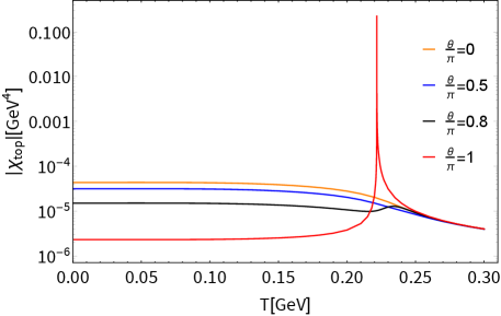
The dependence of and on is plotted in Fig. 1. The present model yields MeV, which is in good agreement with the lattice estimate, MeV Borsanyi:2016ksw . As seen from the left panel of the figure, prominently gets smaller when , which is due to the suppression of (as shown in Appendix B), instead gets greater than , as was expected from the generic argument in Eq.(7). We also note from Appendix B that the chiral phase transition goes like crossover for any , whereas the CP phase transition is of the second order type at (see Fig. 1), which is also manifested as a spike structure of . In particular, the CP symmetry is restored at the criticality ( MeV) in accordance with the literature Boer:2008ct ; Boomsma:2009eh ; Sakai:2011gs .
We assume that an ALP has already been present before the QCD phase transition epoch as in the literature Li:2024psa ; Ellis:2023oxs ; Lozanov:2023rcd ; Gelmini:2023kvo ; Kitajima:2023cek ; Geller:2023shn ; Bai:2023cqj ; Blasi:2023sej and developed the potential having the shift symmetry, with being integer:
| (8) |
where and are the ALP mass and decay constant, respectively. Then a domain wall profile exists as a soliton solution, which sweeps between the adjacent vacua, where in above corresponds to the domain wall number. As the universe cools down to the QCD scale, assuming existence of the ALP coupling to gluon fields, the ALP develops another potential via the axial anomaly,
| (9) |
which explicitly breaks the original shift symmetry, where is some factor related to and highly depending on the Peccei-Quinn charges of quarks. The original ALP vacuum-potential energy is assumed to be . Thus the domain wall configuration, which is supported by the original shift symmetry, becomes unstable in the total ALP potential :
| (10) |
with the normalization . Meanwhile, the domain wall network (with ) starts to collapse and release the latent heat into the universe. Here, plays the role of what is called the bias, . The released energy density can be evaluated by the vacuum energy at the original vacua . For instance, when , the original vacuum at gets the energy shift by :
| (11) |
Thus one may maximally have the released latent heat
| (12) |
Similar discussions have been made in the literature Li:2024psa ; Ellis:2023oxs ; Lozanov:2023rcd ; Gelmini:2023kvo ; Kitajima:2023cek ; Geller:2023shn ; Bai:2023cqj ; Blasi:2023sej . A more precise estimate based on the numerical simulations of the domain wall network suggests Saikawa:2017hiv ; Hiramatsu:2010yz ; Hiramatsu:2012sc ; Hiramatsu:2013qaa .
The QCD bias generically does not significantly affect the ALP potential when the universe is hotter than the QCD scale of MeV, as seen from Fig. 1 and also from the generic formula in Eq.(4). This is essentially due to the correlation of the effective restoration of the chiral (via ) and/or axial symmetry () at higher temperatures (See Eq.(4)). We assume that the ALP-domain wall annihilation takes place at by the QCD bias and fully provides the source of the GW #4#4#4 The ALP domain wall network will completely be decayed never to be left before the expected domain wall-dominated epoch arises. The critical temperature for the domain wall domination is estimated by using the present NJL model and evaluating the condition , to give MeV, which is indeed much lower than the QCD scale. . The produced GW power spectrum at the peak frequency is then assessed via the signal strength, free from the domain wall string tension , by the following signal strength (see, e.g., Blasi:2023sej ):
| (13) |
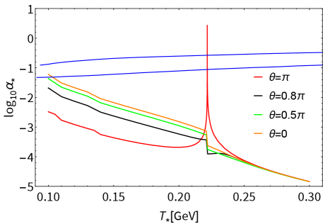
where we have used Saikawa:2017hiv ; Hiramatsu:2010yz ; Hiramatsu:2012sc ; Hiramatsu:2013qaa and . This has been constrained by the NANOGrav 15yr data set as a function of . See Fig. 2, showing that the cases with are incompatible with the interpretation of the NANOGrav 15-year data at around MeV. This is essentially due to the suppression of the scalar quark condensate as observed in as shown in Fig. 1. At onset the criticality (at MeV), the signal gets dramatically enhanced by the singular spike structure reflecting the second order phase transition of the CP symmetry, which is, however, to be too big to interpret the data. This feature is insensitive to the deconfinement phase transition of QCD, which has not yet been incorporated in the figure.
IV Summary and discussions
In summary,
the ALP domain wall with
a QCD bias may be incompatible with the NANOGrav 15-year data on a stochastic GW background, when
the domain wall network collapses in the hot-QCD induced local-CP odd domain
which could allow to have a sizable QCD parameter.
This is due to the drastic suppression of the QCD bias set by
the QCD topological susceptibility, , in the presence of the CP-odd domain
with (see Eq.(7) and Fig. 1).
An explicit model analysis of with a large
based on the two-flavor NJL model implies
that only at , the QCD bias tends to get
significantly large enough due to the criticality of the thermal CP restoration.
However, this turned out to give too big signal strengths to be consistent with
the NANOGrav 15-year data.
In closing, we give several comments on the issues to be pursed in the future.
-
•
The presently employed MFA of NJL model does not precisely reproduce the chiral crossover at as has been observed in the lattice simulations. The latter predicts the pseudocritical temperature MeV Aoki:2009sc ; Borsanyi:2011bn ; Ding:2015ona ; Bazavov:2018mes ; Ding:2020rtq , while the present model yields MeV. This may imply a simple shift of the -distribution of in Fig. 1 and also toward lower with lower criticality, say, at MeV. Even in that case, however, the trend of the dramatic suppression of with should keep manifest for below the shifted criticality ( MeV) and the spike signal associated with the strong CP restoration at will be left at the criticality.
-
•
In Appendix B we have also taken into account a sort of the QCD deconfinement phase transition by extending the NJL model into the Polyakov-loop NJL (PNJL) model Fukushima:2003fw (for a recent review, see, e.g., Fukushima:2017csk ). It turns out that the high suppression of with is still manifest and the presence of a sharp spike in at still persists, in accord with the earlier work Sakai:2011gs . This implies the insensitivity of the deconfinement-confinement transition for the main conclusion addressed in the main text.
-
•
The local CP-odd domain would generate not only a large , but also the fluctuation of in the temporal direction, , which is identified as the so-called chiral chemical potential (often denoted as ) Kharzeev:2007tn ; Kharzeev:2007jp ; Fukushima:2008xe . The contribution to the thermal chiral phase transition as well as has been discussed in Ref. Ruggieri:2020qtq based on a two-flavor NJL model with . From the reference we can see that a part of , which only includes the scalar condensate term as in Eq.(6) (without the contribution in Eq.(4)), roughly gets enhanced by about a factor of at around MeV. With , the scalar condensate generically gets smaller due to the CP violation as in the generic argument (Sec. II), which still holds even in the presence of because does not modify the mixture structure between and as in Eq.(2). Furthermore, the presence of as well as nonzero does not change the form of all the anomalous chiral Ward-identities as clarified in Appendix A. Hence the high suppression of would still be seen even with , so the conclusion as presently claimed would be intact. More precise discussions including the size of the spike at would be worth pursing elsewhere.
-
•
The criticality associated with the thermal CP restoration at would be crucial to precisely check if the ALP domain wall annihilation can still be viable to account for the NANOGrav 15-year data. The related spike structure, following the order of the phase transition, the first order or the second order, would be subject to effective model approaches for QCD Dashen:1970et ; Witten:1980sp ; Pisarski:1996ne ; Creutz:2003xu ; Mizher:2008hf ; Boer:2008ct ; Creutz:2009kx ; Boomsma:2009eh ; Sakai:2011gs ; Chatterjee:2011yz ; Sasaki:2011cj ; Sasaki:2013ewa ; Aoki:2014moa ; Gaiotto:2017tne ; Verbaarschot:2014upa ; Gaiotto:2017yup ; Bai:2023cqj . The presently employed NJL-type model with the MFA tends to predict the second order Boer:2008ct ; Boomsma:2009eh ; Sakai:2011gs , while the linear-sigma model type with the MFA Pisarski:1996ne ; Creutz:2003xu ; Mizher:2008hf ; Boer:2008ct ; Creutz:2009kx ; Boomsma:2009eh ; Bai:2023cqj and the ‘t Hooft anomaly matching argument Gaiotto:2017tne ; Gaiotto:2017yup supports the first order phase transition. Even going beyond the MFA and/or the RPA, including subleading order contributions in expansion, the presently claimed incompatibility would be crucial to deduce a more definite conclusion of the compatibility of the ALP domain wall interpretation with NANOGrav 15-year data. The functional renormalization group analysis makes it possible to clarify the case, which deserves to another publication. At any rate, the presently claimed incompatibility would still pin down one benchmark point in the full parameter space of the QCD-biased ALP domain wall collapse.
-
•
As seen from Figs. 3 and 4 in Appendix B, at the thermal CP restoration point coincides with the pseudocritical point (inflection point) for the chiral crossover. This is due to the present MFA, which involves the two intrinsic features at : i) the chiral symmetry is not spontaneously broken via the scalar quark condensate , as long as the CP symmetry is broken; ii) no axial violating loop corrections are generated at this approximation level. Those lead to no thermal development of until the CP symmetry restores, hence gets kicked down instantaneously, i.e., undergoes the pseudocritical point at the same timing as the CP restoration. We have clarified those points in Appendix B (around Eq.(61)). Going beyond the MFA analysis, such as the functional renormalization group, would potentially generate a gap between two critical points for the (effective) chiral and CP symmetry restorations, which should come from the axial anomaly effects in loops. The further investigation along this line could also make a complementary benchmark compared to the prediction from the ‘t Hooft-anomaly matching in pure Yang-Mills theories Chen:2020syd , which suggests the CP restoration temperature is higher than or equal to the deconfinement phase transition one.
-
•
When strange quark contributions are incorporated in the analysis, the thermal CP restoration at would be more involved. First of all, one notices that the CP phase contribution carried by the strange quark is highly suppressed by a factor of , as reviewed in Appendix A (around Eqs.(23) - (25)). This observation comes from the robust flavor singlet nature of the dependence in QCD that requires the strange quark field to carry the phase with the form , i.e., almost free from . Thus, as far as the CP violating effects are concerned, the three-flavor QCD is essentially decomposed into the (the lightest two quarks and the strange quark) structure and the CP order parameter is almost controlled by the lightest two-flavor sector, i.e., .
This is the characteristic flavor violation and irrespective to the presence of the QCD topological charge fluctuation, which is flavor universal, or equivalently in the NJL framework, the ‘t Hooft-Kobayashi-Maskawa determinant term Kobayashi:1970ji ; Kobayashi:1971qz ; tHooft:1976rip ; tHooft:1976snw (as in Appendix B). In the three-flavor NJL with the MFA, thus the chiral crossover for would still persist even at , simply because of presence of the finite strange quark mass, while would be subject to the approximation for QCD, or the (P)NJL. In the MFA of the three-flavor NJL, would be trapped to a constant value until the CP phase transition takes place at , and then starts to drops when (with discontinuity in the -derivative at ), as in the two-flavor case (Fig. 3 in Appendix B). As in the case with , would drop down with more slowly than simply due to the larger strange quark mass. Thus, in the framework of the MFA of the NJL, the CP phase transition in the three-flavor case would be essentially identical to the one in the lightest two-flavor case, hence it would still be of the second order keeping the critical spike structure of , hence does as well, as seen from Fig. 2.
However, as has been discussed in the recent literature Fejos:2016hbp ; Fejos:2023lvw ; Fejos:2021yod based on the functional renormalization group analysis on the three-flavor linear sigma model with , the ‘t Hooft-Kobayashi-Maskawa determinant term beyond the MFA could be nonperturbatively enhanced at around even in the case of . This implies that the criticality of the CP phase transition as well as the chiral phase transition might significantly be altered and the entry of the strange quark contributions beyond the MFA might be nontrivial, though the carried CP phase is intrinsically highly suppressed as aforementioned. Thus, the detailed analysis in the three-flavor NJL, both within and beyond the MFA, is noteworthy to pursue in another publication.
Finally, we comment on impacts of lattice QCD calculations to this observation. Most of current lattice QCD calculations at the physical point have been done using the Monte-Carlo method. For nonzero theta, simulations are suffered from infamous sign problem. Namely, we cannot calculate expectation values with . To avoid the problem in the realistic setup, we employ imaginary theta and analytic continue to the real theta to get expectation values for physical observables DelDebbio:2002xa ; DElia:2003zne ; DelDebbio:2006sbu ; Giusti:2007tu ; Izubuchi:2007rmy ; Vicari:2008jw ; DElia:2013uaf ; Hirasawa:2024vns . These calculations for have been done away from the physical point. An interesting methods for nonzero theta is suggested Kitano:2021jho , but it is still hard to get physical results. Digital and analog quantum simulations and calculations with nonzero theta using tensor networks have been performed for toy models but not for the realistic setup like four dimensional QCD at the physical point Byrnes:2002gj ; Funcke:2019zna ; Kuramashi:2019cgs ; Chakraborty:2020uhf ; Honda:2021aum ; Honda:2022hyu .
Acknowledgments
We are grateful to Taishi Katsuragawa and Wen Yin for useful comments. This work was supported in part by the National Science Foundation of China (NSFC) under Grant No.11747308, 11975108, 12047569, and the Seeds Funding of Jilin University (S.M.), and Toyama First Bank, Ltd (H.I.). The work by M.K. was supported by the Fundamental Research Funds for the Central Universities and partially by the National Natural Science Foundation of China (NSFC) Grant No. 12235016, and the Strategic Priority Research Program of Chinese Academy of Sciences under Grant No. XDB34030000. The work of A.T. was partially supported by JSPS KAKENHI Grant Numbers 20K14479, 22K03539, 22H05112, and 22H05111, and MEXT as “Program for Promoting Researches on the Supercomputer Fugaku” (Simulation for basic science: approaching the new quantum era; Grant Number JPMXP1020230411, and Search for physics beyond the standard model using large-scale lattice QCD simulation and development of AI technology toward next-generation lattice QCD; Grant Number JPMXP1020230409).
Appendix A Generic properties of anomalous chiral Ward-Takahashi identities (ACWTIs) in QCD
A.1 ACWTIs with external gauge fields and
We start with the QCD Lagrangian with quarks including the external gauge fields,
| (14) |
where denotes the left-(right-) handed quark fields belong to the fundamental representation of ; is the current quark mass for -quark taking the diagonal form like ; are the field strengths of the gluon fields ; stand for the generators of the QCD color group ; denotes the QCD gauge coupling constant; plays the role of the source for the topological operator ; The external gauge fields and () are introduced by gauging the global chiral and symmetry, which are embedded into the covariant derivatives as
| (15) |
with being the generators of in the flavor space.
The vacuum energy of QCD is given by
| (16) |
where represents the generating functional of QCD in Minkowski spacetime,
| (17) |
We define the topological susceptibility including the dependence:
| (18) | |||||
where we have introduced the subscript to explicitize the dependence on the vacuum.
The external fields, such as the electromagnetic field , the baryon chemical potential , and the chiral chemical potential , are embedded in the external gauge fields as #5#5#5 The isospin chemical potential can also be incorporated, when , into the covariant derivative as an additional external gauge field term proportional to .
| (19) |
where represents the electromagnetic coupling constant, and denotes the electric charge matrix for quarks . The chemical potentials have been introduced as constant fields. In QCD with the external gauge fields, the symmetry is explicitly broken by the current quark mass term and the gluonic quantum anomaly, and also external electromagnetic field. This is reflected in the anomalous conservation law of the axial current for each quark in the -plet quark field , labeled as ,
| (20) |
with the axial current . Note that the constant chemical potentials do not contribute to the anomalous conservation law.
Under the rotation with the rotation angle , the quark fields transform as
| (21) |
Then the QCD generating functional gets shifted as
| (22) |
To rotate the QCD term away, we take the following phase choice reflecting the flavor-singlet nature of the QCD vacuum Kawaguchi:2020kdl ; Kawaguchi:2020qvg ; Cui:2021bqf ; Cui:2022vsr ,
| (23) |
with
| (24) |
Then the QCD generating functional goes like
| (25) | |||||
From this generating functional, the topological susceptibility is given as
| (26) |
where
| (27) | |||||
These susceptibilities are written in terms of the primed quark field . They can be rewritten in terms of the original quark field using the following connection,
| (28) |
Then and go like
| (29) |
The term in Eq.(26) is precisely the generalization of the one in Eq.(4) with Eq.(5), which has also been addressed in the literature Kawaguchi:2020kdl ; Kawaguchi:2020qvg ; Cui:2021bqf ; Cui:2022vsr without external gauge fields. Thus the presence of the electromagnetic axial anomaly yields additional topological susceptibility, .
Next, we evaluate the ACWTIs for transformation in QCD. Under the chiral transformation, the quark field transforms as
| (30) |
Then, the chiral transformation of the expectation value for an arbitrary local operator in the path integral formalism yields the ACWTIs:
| (31) |
where denotes the chiral current, , and
| (32) |
with . Equation (31) is a generalization of the ACWTIs addressed in Kawaguchi:2020kdl ; Kawaguchi:2020qvg ; Cui:2021bqf ; Cui:2022vsr without external gauge fields. Unless external gauge fields possess a topologically nontrivial configuration, we can rewrite the covariant derivative term as
| (33) |
Thus we eventually have
| (34) |
This implies that the ACWTIs keep the same form as those in the case without external gauge fields Kawaguchi:2020kdl ; Kawaguchi:2020qvg ; Cui:2021bqf ; Cui:2022vsr .
For instance, in the case of , we find the same form of the ACWTIs as in the literature GomezNicola:2016ssy ; Kawaguchi:2020qvg ; Cui:2021bqf ; Cui:2022vsr :
| (35) |
with . Here denotes the pion susceptibility defined as
| (36) |
with being the connected part of the correlation function, and the pseudoscalar susceptibilities , and are defined as
| (37) |
in Eq.(29) then takes a couple of equivalent forms, related each other by the ACWTIs in Eq.(35) Kawaguchi:2020kdl ; Kawaguchi:2020qvg ; Cui:2021bqf ; Cui:2022vsr
| (38) |
with . It is interesting to note that and are related not to the full topological susceptibility , but , in Eq.(26).
A.2 Renormalization group invariance of
The current quark mass parameter is multiplicatively renormalized as
| (39) |
where denotes the bare cutoff and the upper script stands for the quantity renormalized at the scale . When the mass independent renormalization is thus applied. the renormalization factor is flavor universal. Then we are allowed to drop the flavor label as
| (40) |
This also implies that is independent of the current quark mass as well.
The bilinear operator is also multiplicatively renormalized by ,
| (41) |
so that we have the renormalization group invariant mass term like
| (42) |
Consider also a () operator to be renormalized in a similar way with the renormalization constant
| (43) |
Since none of quark mass dependence is generated in the mass independent renormalization, the axial invariance keeps manifest between renormalization of the () and () operators. Hence we have
| (44) |
In that case we also find
| (45) |
Now, we apply the renormalization procedure as above to in the three-flavor case (Eq.(38)):
| (46) | |||||
Thus it has been proven that is renormalization group invariant. Note that this argument is also applicable to the case with nonzero , because the QCD is itself conventionally renormalization group invariant and no new divergent terms induced due to nonzero will be generated, hence the renormalization factors will not be corrected. Furthermore, one can readily see that the external gauge-induced , defined as in Eq.(27), is also manifestly renormalization group invariant.
Appendix B The details on the (P) NJL model analysis
B.1 NJL case
Our reference NJL Lagrangian with two flavors (up and down quarks) and nonzero follows the literature Sakai:2011gs , which takes the form
| (47) |
where and the determinant acts on the quark flavors. The term, called the ‘t Hooft-Kobayashi-Maskawa determinant term Kobayashi:1970ji ; Kobayashi:1971qz ; tHooft:1976rip ; tHooft:1976snw , breaks axial symmetry, but keeps symmetry, while others keep the full chiral symmetry. The term thus serves as the axial anomaly:
| (48) |
Since the axial symmetry is broken only by and the quark mass terms, one can move in the term to the mass term by a axial rotation as was done in the case of the general argument above:
| (49) |
so that
| (50) |
where
| (51) |
in which nonzero manifestly signals the CP violation. Use of this ”prime” basis is convenient to analyze the model because all the dependence is transformed and collected into the complex mass in the quark propagator. Similarly to Eq.(1), Eq.(49) relates the scalar and pseudoscalar bilinears between the original- and prime-base scalar and pseudoscalar bilinears (for each quark flavor ) as
| (52) |
We work in the MFA, so that the scalar and pseudoscalar bilinears and are expanded around the means fields and , as and , where the terms sandwiched by “” stand for the normal ordered product, meaning that for . Then the interaction terms in Eq.(47) are replaced, up to the normal ordered terms, as
| (53) |
In the MFA the NJL Lagrangian in Eq.(47) thus takes the form
| (54) |
with
| (55) |
Integrating out quarks leads to the thermodynamic potential in the MFA:
| (56) |
where and , and
| (57) |
with . Then and are determined through the stationary condition,
| (58) |
Of particular interest is to see the thermodynamic potential at ,
| (59) |
where things have been written in terms of and by means of Eq.(55). In the presently applied MFA, the loop corrections (corresponding to the last term in Eq.(59)) are axial invariant, i.e., do not separate and due to no loop contributions involving vertices with the determinant coupling . At , the explicit-chiral breaking-effect (by ) has completely been transported into the direction (the second term). The stationary condition then takes the form
| (60) |
When , i.e., the CP symmetry is spontaneously broken, the gap equation for can be rewritten by eliminating the loop correction part as
| (61) | |||||
This implies that in the CP broken phase at , the chiral symmetry is not spontaneously broken and the chiral order parameter does not evolve in .
We come back to the case with arbitrary and derive relevant formulae for the susceptibilities and within the MFA. First, by noting the change of basis in Eq.(52), the susceptibility in of Eq.(4) is written in terms of the prime base as
| (62) |
The “primed” meson susceptibilities are evaluated in the so-called random phase approximation (the bubble-ring resummation ansatz) as
| (63) |
where
| (66) | ||||
| (69) | ||||
| (74) |
with the vacuum polarization functions for each channel,
| (75) |
In evaluating the vacuum polarization functions, we have regularized the 3-momentum integrals by the cutoff .
Putting all the relevant things above into in Eq.(4), we compute as a function of and . The model parameter setting follows the literature Boer:2008ct ; Boomsma:2009eh ; Sakai:2011gs :
| (76) |
The coupling has been related by to the coupling just in a numerical manner, though the associated asymmetry features are different.
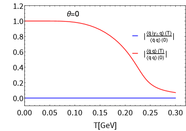
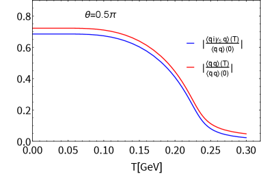
See Fig. 3, where we observe several characteristic features: i) the scalar condensate becomes dramatically smaller with increasing , so that in Eq.(4) gigantically decreases; ii) at , the pseudoscalar condensate undergoes the CP symmetry restoration of the second order type, which generates a significant spike at the criticality in ; iii) at , the scalar condensate does not evolve in at all until the the CP symmetry is restored, in agreement with the analytic discussion around Eq.(61).
B.2 PNJL case
By extending the NJL detailed in the previous subsection into the PNJL model in the MFA following the procedure in the literature Fukushima:2003fw (for a recent review, see, e.g., Fukushima:2017csk ), we have the thermodynamic potential:
| (77) |
where , in which we have introduced the Polyakov loop field with the charges ; the constraint taken into account; takes the same form as in Eq.(57), but would depend on the Polyakov-loop fields and through the stationary condition as in Eq.(58). The Polyakov loop potential is assumed to take the form of polynomial type or logarithmic type:
| (78) |
with
| (79) |
The Polyakov-loop potential parameters are fixed by fitting the lattice data in the pure Yang-Mills theory as Roessner:2006xn ; Ratti:2005jh
| (82) |
The thermodynamic potential in Eq.(77) is thus minimized also with respect to and , in addition to the stationary condition along and directions as in the NJL case, Eq.(76).
In the RPA the following replacement rule for in Eq.(75) due to the Polyakov-loop contribution is applied:
| (83) |
Similarly for an in Eq.(75), we have
| (84) |
Those modified integral functions are precisely reduced back to the ones in Eq.(75) when (without confinement).
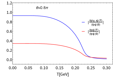
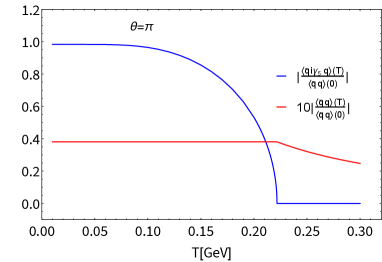
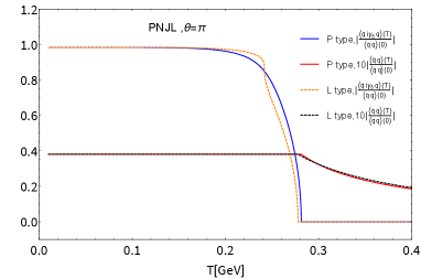
In Fig. 4 we plot the scalar and pseudoscalar condensates, and , as a function of temperature with , and 1. The scalar condensate decreases sharply with increasing . The pseudoscalar condensate undergoes a second-order phase transition at the critical temperature when , and the CP symmetry is restored, which coincides with the NJL case (Fig. 3). At , the scalar condensate does not evolve in at all until the CP symmetry is restored at the critical temperature, in the same way as in the NJL case (Fig. 3) due to the same form of the gap equations as in Eq.(61) because incorporation of the Polyakov loop field does not break the axial symmetry. This is the characteristic MFA feature, which persists both in the NJL and PNJL cases.
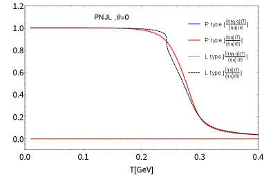
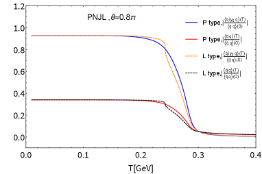
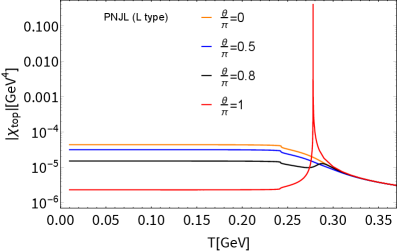
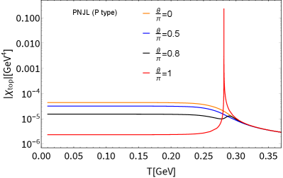
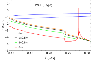
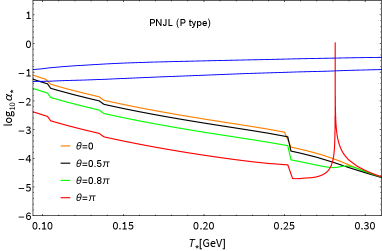
Those universal trends have also been seen in , in Fig. 5, which shows no substantial difference from the case of the NJL as in Fig. 1, hence the dramatic suppression of around MeV still persists for even with the PL contribution taken into account (See Fig. 6). At , the peak signal strengths in the PNJL model (whichever type L or P) deviates from the 2 contour, as has also been observed in the NJL case (Fig. 2 in the main text).

References
- (1) G. Agazie et al. [NANOGrav], Astrophys. J. Lett. 951, no.1, L8 (2023) doi:10.3847/2041-8213/acdac6 [arXiv:2306.16213 [astro-ph.HE]].
- (2) G. Agazie et al. [NANOGrav], Astrophys. J. Lett. 952, no.2, L37 (2023) doi:10.3847/2041-8213/ace18b [arXiv:2306.16220 [astro-ph.HE]].
- (3) A. Afzal et al. [NANOGrav], Astrophys. J. Lett. 951, no.1, L11 (2023) doi:10.3847/2041-8213/acdc91 [arXiv:2306.16219 [astro-ph.HE]].
- (4) J. Antoniadis et al. [EPTA], Astron. Astrophys. 678, A48 (2023) doi:10.1051/0004-6361/202346841 [arXiv:2306.16224 [astro-ph.HE]].
- (5) J. Antoniadis et al. [EPTA and InPTA], Astron. Astrophys. 678, A49 (2023) doi:10.1051/0004-6361/202346842 [arXiv:2306.16225 [astro-ph.HE]].
- (6) J. Antoniadis et al. [EPTA and InPTA:], Astron. Astrophys. 678, A50 (2023) doi:10.1051/0004-6361/202346844 [arXiv:2306.16214 [astro-ph.HE]].
- (7) D. J. Reardon, A. Zic, R. M. Shannon, G. B. Hobbs, M. Bailes, V. Di Marco, A. Kapur, A. F. Rogers, E. Thrane and J. Askew, et al. Astrophys. J. Lett. 951, no.1, L6 (2023) doi:10.3847/2041-8213/acdd02 [arXiv:2306.16215 [astro-ph.HE]].
- (8) D. J. Reardon, A. Zic, R. M. Shannon, V. Di Marco, G. B. Hobbs, A. Kapur, M. E. Lower, R. Mandow, H. Middleton and M. T. Miles, et al. Astrophys. J. Lett. 951, no.1, L7 (2023) doi:10.3847/2041-8213/acdd03 [arXiv:2306.16229 [astro-ph.HE]].
- (9) H. Xu, S. Chen, Y. Guo, J. Jiang, B. Wang, J. Xu, Z. Xue, R. N. Caballero, J. Yuan and Y. Xu, et al. Res. Astron. Astrophys. 23, no.7, 075024 (2023) doi:10.1088/1674-4527/acdfa5 [arXiv:2306.16216 [astro-ph.HE]].
- (10) H. J. Li and Y. F. Zhou, [arXiv:2401.09138 [hep-ph]].
- (11) J. Ellis, M. Fairbairn, G. Franciolini, G. Hütsi, A. Iovino, M. Lewicki, M. Raidal, J. Urrutia, V. Vaskonen and H. Veermäe, Phys. Rev. D 109, no.2, 023522 (2024) doi:10.1103/PhysRevD.109.023522 [arXiv:2308.08546 [astro-ph.CO]].
- (12) K. D. Lozanov, S. Pi, M. Sasaki, V. Takhistov and A. Wang, [arXiv:2310.03594 [astro-ph.CO]].
- (13) G. B. Gelmini and J. Hyman, Phys. Lett. B 848, 138356 (2024) doi:10.1016/j.physletb.2023.138356 [arXiv:2307.07665 [hep-ph]].
- (14) N. Kitajima, J. Lee, K. Murai, F. Takahashi and W. Yin, Phys. Lett. B 851, 138586 (2024) doi:10.1016/j.physletb.2024.138586 [arXiv:2306.17146 [hep-ph]].
- (15) M. Geller, S. Ghosh, S. Lu and Y. Tsai, Phys. Rev. D 109, no.6, 063537 (2024) doi:10.1103/PhysRevD.109.063537 [arXiv:2307.03724 [hep-ph]].
- (16) Y. Bai, T. K. Chen and M. Korwar, JHEP 12, 194 (2023) doi:10.1007/JHEP12(2023)194 [arXiv:2306.17160 [hep-ph]].
- (17) S. Blasi, A. Mariotti, A. Rase and A. Sevrin, JHEP 11, 169 (2023) doi:10.1007/JHEP11(2023)169 [arXiv:2306.17830 [hep-ph]].
- (18) S. Borsanyi, Z. Fodor, J. Guenther, K. H. Kampert, S. D. Katz, T. Kawanai, T. G. Kovacs, S. W. Mages, A. Pasztor and F. Pittler, et al. Nature 539, no.7627, 69-71 (2016) doi:10.1038/nature20115 [arXiv:1606.07494 [hep-lat]].
- (19) N. S. Manton, Phys. Rev. D 28, 2019 (1983) doi:10.1103/PhysRevD.28.2019
- (20) F. R. Klinkhamer and N. S. Manton, Phys. Rev. D 30, 2212 (1984) doi:10.1103/PhysRevD.30.2212
- (21) D. Kharzeev and A. Zhitnitsky, Nucl. Phys. A 797, 67-79 (2007) doi:10.1016/j.nuclphysa.2007.10.001 [arXiv:0706.1026 [hep-ph]].
- (22) D. E. Kharzeev, L. D. McLerran and H. J. Warringa, Nucl. Phys. A 803, 227-253 (2008) doi:10.1016/j.nuclphysa.2008.02.298 [arXiv:0711.0950 [hep-ph]].
- (23) K. Fukushima, D. E. Kharzeev and H. J. Warringa, Phys. Rev. D 78, 074033 (2008) doi:10.1103/PhysRevD.78.074033 [arXiv:0808.3382 [hep-ph]].
- (24) L. D. McLerran, E. Mottola and M. E. Shaposhnikov, Phys. Rev. D 43, 2027-2035 (1991) doi:10.1103/PhysRevD.43.2027
- (25) G. D. Moore, Phys. Lett. B 412, 359-370 (1997) doi:10.1016/S0370-2693(97)01046-0 [arXiv:hep-ph/9705248 [hep-ph]].
- (26) G. D. Moore and K. Rummukainen, Phys. Rev. D 61, 105008 (2000) doi:10.1103/PhysRevD.61.105008 [arXiv:hep-ph/9906259 [hep-ph]].
- (27) D. Bodeker, G. D. Moore and K. Rummukainen, Phys. Rev. D 61, 056003 (2000) doi:10.1103/PhysRevD.61.056003 [arXiv:hep-ph/9907545 [hep-ph]].
- (28) A. A. Andrianov, V. A. Andrianov, D. Espriu and X. Planells, Phys. Lett. B 710, 230-235 (2012) doi:10.1016/j.physletb.2012.02.072 [arXiv:1201.3485 [hep-ph]].
- (29) A. A. Andrianov, D. Espriu and X. Planells, Eur. Phys. J. C 73, no.1, 2294 (2013) doi:10.1140/epjc/s10052-013-2294-0 [arXiv:1210.7712 [hep-ph]].
- (30) M. Kawaguchi, S. Matsuzaki and A. Tomiya, Phys. Rev. D 103, no.5, 054034 (2021) doi:10.1103/PhysRevD.103.054034 [arXiv:2005.07003 [hep-ph]].
- (31) C. X. Cui, J. Y. Li, S. Matsuzaki, M. Kawaguchi and A. Tomiya, Phys. Rev. D 105, no.11, 114031 (2022) doi:10.1103/PhysRevD.105.114031 [arXiv:2106.05674 [hep-ph]].
- (32) C. X. Cui, J. Y. Li, S. Matsuzaki, M. Kawaguchi and A. Tomiya, Particles 7, no.1, 237-263 (2024) doi:10.3390/particles7010014 [arXiv:2205.12479 [hep-ph]].
- (33) H. Leutwyler and A. V. Smilga, Phys. Rev. D 46, 5607-5632 (1992) doi:10.1103/PhysRevD.46.5607
- (34) M. Kawaguchi, S. Matsuzaki and A. Tomiya, Phys. Lett. B 813, 136044 (2021) doi:10.1016/j.physletb.2020.136044 [arXiv:2003.11375 [hep-ph]].
- (35) R. F. Dashen, Phys. Rev. D 3, 1879-1889 (1971) doi:10.1103/PhysRevD.3.1879
- (36) E. Witten, Annals Phys. 128, 363 (1980) doi:10.1016/0003-4916(80)90325-5
- (37) R. D. Pisarski, Phys. Rev. Lett. 76, 3084-3087 (1996) doi:10.1103/PhysRevLett.76.3084 [arXiv:hep-ph/9601316 [hep-ph]].
- (38) M. Creutz, Phys. Rev. Lett. 92, 201601 (2004) doi:10.1103/PhysRevLett.92.201601 [arXiv:hep-lat/0312018 [hep-lat]].
- (39) A. J. Mizher and E. S. Fraga, Nucl. Phys. A 831, 91-105 (2009) doi:10.1016/j.nuclphysa.2009.09.004 [arXiv:0810.5162 [hep-ph]].
- (40) D. Boer and J. K. Boomsma, Phys. Rev. D 78, 054027 (2008) doi:10.1103/PhysRevD.78.054027 [arXiv:0806.1669 [hep-ph]].
- (41) M. Creutz, Annals Phys. 324, 1573-1584 (2009) doi:10.1016/j.aop.2009.01.005 [arXiv:0901.0150 [hep-ph]].
- (42) J. K. Boomsma and D. Boer, Phys. Rev. D 80, 034019 (2009) doi:10.1103/PhysRevD.80.034019 [arXiv:0905.4660 [hep-ph]].
- (43) Y. Sakai, H. Kouno, T. Sasaki and M. Yahiro, Phys. Lett. B 705, 349-355 (2011) doi:10.1016/j.physletb.2011.10.032 [arXiv:1105.0413 [hep-ph]].
- (44) B. Chatterjee, H. Mishra and A. Mishra, Phys. Rev. D 85, 114008 (2012) doi:10.1103/PhysRevD.85.114008 [arXiv:1111.4061 [hep-ph]].
- (45) T. Sasaki, J. Takahashi, Y. Sakai, H. Kouno and M. Yahiro, Phys. Rev. D 85, 056009 (2012) doi:10.1103/PhysRevD.85.056009 [arXiv:1112.6086 [hep-ph]].
- (46) T. Sasaki, H. Kouno and M. Yahiro, Phys. Rev. D 87, no.5, 056003 (2013) doi:10.1103/PhysRevD.87.056003 [arXiv:1208.0375 [hep-ph]].
- (47) S. Aoki and M. Creutz, Phys. Rev. Lett. 112, no.14, 141603 (2014) doi:10.1103/PhysRevLett.112.141603 [arXiv:1402.1837 [hep-lat]].
- (48) K. Mameda, Nucl. Phys. B 889, 712-726 (2014) doi:10.1016/j.nuclphysb.2014.11.002 [arXiv:1408.1189 [hep-ph]].
- (49) J. J. M. Verbaarschot and T. Wettig, Phys. Rev. D 90, no.11, 116004 (2014) doi:10.1103/PhysRevD.90.116004 [arXiv:1407.8393 [hep-th]].
- (50) D. Gaiotto, Z. Komargodski and N. Seiberg, JHEP 01, 110 (2018) doi:10.1007/JHEP01(2018)110 [arXiv:1708.06806 [hep-th]].
- (51) D. Gaiotto, A. Kapustin, Z. Komargodski and N. Seiberg, JHEP 05, 091 (2017) doi:10.1007/JHEP05(2017)091 [arXiv:1703.00501 [hep-th]].
- (52) G. ’t Hooft, NATO Sci. Ser. B 59, 135-157 (1980) doi:10.1007/978-1-4684-7571-5_9
- (53) Y. Frishman, A. Schwimmer, T. Banks and S. Yankielowicz, Nucl. Phys. B 177, 157-171 (1981) doi:10.1016/0550-3213(81)90268-6
- (54) K. Saikawa, Universe 3, no.2, 40 (2017) doi:10.3390/universe3020040 [arXiv:1703.02576 [hep-ph]].
- (55) T. Hiramatsu, M. Kawasaki and K. Saikawa, JCAP 05, 032 (2010) doi:10.1088/1475-7516/2010/05/032 [arXiv:1002.1555 [astro-ph.CO]].
- (56) T. Hiramatsu, M. Kawasaki, K. Saikawa and T. Sekiguchi, JCAP 01, 001 (2013) doi:10.1088/1475-7516/2013/01/001 [arXiv:1207.3166 [hep-ph]].
- (57) T. Hiramatsu, M. Kawasaki and K. Saikawa, JCAP 02, 031 (2014) doi:10.1088/1475-7516/2014/02/031 [arXiv:1309.5001 [astro-ph.CO]].
- (58) R. L. Workman et al. [Particle Data Group], PTEP 2022, 083C01 (2022) doi:10.1093/ptep/ptac097
- (59) Y. Aoki, S. Borsanyi, S. Durr, Z. Fodor, S. D. Katz, S. Krieg and K. K. Szabo, JHEP 06, 088 (2009) doi:10.1088/1126-6708/2009/06/088 [arXiv:0903.4155 [hep-lat]].
- (60) S. Borsanyi et al. [Wuppertal-Budapest], J. Phys. Conf. Ser. 316, 012020 (2011) doi:10.1088/1742-6596/316/1/012020 [arXiv:1109.5032 [hep-lat]].
- (61) H. T. Ding, F. Karsch and S. Mukherjee, Int. J. Mod. Phys. E 24, no.10, 1530007 (2015) doi:10.1142/S0218301315300076 [arXiv:1504.05274 [hep-lat]].
- (62) A. Bazavov et al. [HotQCD], Phys. Lett. B 795, 15-21 (2019) doi:10.1016/j.physletb.2019.05.013 [arXiv:1812.08235 [hep-lat]].
- (63) H. T. Ding, Nucl. Phys. A 1005, 121940 (2021) doi:10.1016/j.nuclphysa.2020.121940 [arXiv:2002.11957 [hep-lat]].
- (64) K. Fukushima, Phys. Lett. B 591, 277-284 (2004) doi:10.1016/j.physletb.2004.04.027 [arXiv:hep-ph/0310121 [hep-ph]].
- (65) K. Fukushima and V. Skokov, Prog. Part. Nucl. Phys. 96, 154-199 (2017) doi:10.1016/j.ppnp.2017.05.002 [arXiv:1705.00718 [hep-ph]].
- (66) M. Ruggieri, M. N. Chernodub and Z. Y. Lu, Phys. Rev. D 102, no.1, 014031 (2020) doi:10.1103/PhysRevD.102.014031 [arXiv:2004.09393 [hep-ph]].
- (67) S. Chen, K. Fukushima, H. Nishimura and Y. Tanizaki, Phys. Rev. D 102, no.3, 034020 (2020) doi:10.1103/PhysRevD.102.034020 [arXiv:2006.01487 [hep-th]].
- (68) M. Kobayashi and T. Maskawa, Prog. Theor. Phys. 44, 1422-1424 (1970) doi:10.1143/PTP.44.1422
- (69) M. Kobayashi, H. Kondo and T. Maskawa, Prog. Theor. Phys. 45, 1955-1959 (1971) doi:10.1143/PTP.45.1955
- (70) G. ’t Hooft, Phys. Rev. Lett. 37, 8-11 (1976) doi:10.1103/PhysRevLett.37.8
- (71) G. ’t Hooft, Phys. Rev. D 14, 3432-3450 (1976) [erratum: Phys. Rev. D 18, 2199 (1978)] doi:10.1103/PhysRevD.14.3432
- (72) G. Fejos and A. Hosaka, Phys. Rev. D 94, no.3, 036005 (2016) doi:10.1103/PhysRevD.94.036005 [arXiv:1604.05982 [hep-ph]].
- (73) G. Fejos and A. Patkos, Phys. Rev. D 109, no.3, 036035 (2024) doi:10.1103/PhysRevD.109.036035 [arXiv:2311.02186 [hep-ph]].
- (74) G. Fejös and A. Patkos, Phys. Rev. D 105, no.9, 096007 (2022) doi:10.1103/PhysRevD.105.096007 [arXiv:2112.14903 [hep-ph]].
- (75) L. Del Debbio, H. Panagopoulos and E. Vicari, JHEP 08, 044 (2002) doi:10.1088/1126-6708/2002/08/044 [arXiv:hep-th/0204125 [hep-th]].
- (76) M. D’Elia, Nucl. Phys. B 661, 139-152 (2003) doi:10.1016/S0550-3213(03)00311-0 [arXiv:hep-lat/0302007 [hep-lat]].
- (77) L. Del Debbio, G. M. Manca, H. Panagopoulos, A. Skouroupathis and E. Vicari, PoS LAT2006, 045 (2006) doi:10.22323/1.032.0045 [arXiv:hep-th/0610100 [hep-th]].
- (78) L. Giusti, S. Petrarca and B. Taglienti, Phys. Rev. D 76, 094510 (2007) doi:10.1103/PhysRevD.76.094510 [arXiv:0705.2352 [hep-th]].
- (79) T. Izubuchi, S. Aoki, K. Hashimoto, Y. Nakamura, T. Sekido and G. Schierholz, PoS LATTICE2007, 106 (2007) doi:10.22323/1.042.0106 [arXiv:0802.1470 [hep-lat]].
- (80) E. Vicari and H. Panagopoulos, Phys. Rept. 470, 93-150 (2009) doi:10.1016/j.physrep.2008.10.001 [arXiv:0803.1593 [hep-th]].
- (81) M. D’Elia and F. Negro, Phys. Rev. D 88, no.3, 034503 (2013) doi:10.1103/PhysRevD.88.034503 [arXiv:1306.2919 [hep-lat]].
- (82) M. Hirasawa, K. Hatakeyama, M. Honda, A. Matsumoto, J. Nishimura and A. Yosprakob, PoS LATTICE2023, 193 (2024) doi:10.22323/1.453.0193 [arXiv:2401.05726 [hep-lat]].
- (83) R. Kitano, R. Matsudo, N. Yamada and M. Yamazaki, Phys. Lett. B 822, 136657 (2021) doi:10.1016/j.physletb.2021.136657 [arXiv:2102.08784 [hep-lat]].
- (84) T. Byrnes, P. Sriganesh, R. J. Bursill and C. J. Hamer, Nucl. Phys. B Proc. Suppl. 109, 202-206 (2002) doi:10.1016/S0920-5632(02)01416-0 [arXiv:hep-lat/0201007 [hep-lat]].
- (85) L. Funcke, K. Jansen and S. Kühn, Phys. Rev. D 101, no.5, 054507 (2020) doi:10.1103/PhysRevD.101.054507 [arXiv:1908.00551 [hep-lat]].
- (86) Y. Kuramashi and Y. Yoshimura, JHEP 04, 089 (2020) doi:10.1007/JHEP04(2020)089 [arXiv:1911.06480 [hep-lat]].
- (87) B. Chakraborty, M. Honda, T. Izubuchi, Y. Kikuchi and A. Tomiya, Phys. Rev. D 105, no.9, 094503 (2022) doi:10.1103/PhysRevD.105.094503 [arXiv:2001.00485 [hep-lat]].
- (88) M. Honda, E. Itou, Y. Kikuchi, L. Nagano and T. Okuda, Phys. Rev. D 105, no.1, 014504 (2022) doi:10.1103/PhysRevD.105.014504 [arXiv:2105.03276 [hep-lat]].
- (89) M. Honda, doi:10.1142/9789811261633_0003
- (90) A. Gómez Nicola and J. Ruiz de Elvira, JHEP 03, 186 (2016) doi:10.1007/JHEP03(2016)186 [arXiv:1602.01476 [hep-ph]].
- (91) S. Roessner, C. Ratti and W. Weise, Phys. Rev. D 75, 034007 (2007) doi:10.1103/PhysRevD.75.034007 [arXiv:hep-ph/0609281 [hep-ph]].
- (92) C. Ratti, M. A. Thaler and W. Weise, Phys. Rev. D 73, 014019 (2006) doi:10.1103/PhysRevD.73.014019 [arXiv:hep-ph/0506234 [hep-ph]].