Lattice Parton Collaboration ()
Impact of gauge fixing precision
on the continuum limit
of non-local quark-bilinear lattice operators
Kuan Zhang
Abstract
We analyze the gauge fixing precision dependence of some non-local quark-blinear lattice operators interesting in computing parton physics for several measurements, using 5 lattice spacings ranging from 0.032 fm to 0.121 fm. Our results show that gauge dependent non-local measurements are significantly more sensitive to the precision of gauge fixing than anticipated. The impact of imprecise gauge fixing is significant for fine lattices and long distances. For instance, even with the typically defined precision of Landau gauge fixing of , the deviation caused by imprecise gauge fixing can reach 12 percent, when calculating the trace of Wilson lines at 1.2 fm with a lattice spacing of approximately 0.03 fm. Similar behavior has been observed in gauge and Coulomb gauge as well. For both quasi PDFs and quasi TMD-PDFs operators renormalized using the RI/MOM scheme, convergence for different lattice spacings at long distance is only observed when the precision of Landau gauge fixing is sufficiently high. To describe these findings quantitatively, we propose an empirical formula to estimate the required precision.
I Introduction
In gauge field theories, the necessity of gauge fixing arises originally from perturbation theory. If we just focus on non-perturbative lattice gauge theory and gauge invariant quantities, we do not really need gauge fixing. Also, any gauge dependent quantity will vanish if averaged over a sufficient number of configurations. However, in certain non-perturbative renormalization schemes Martinelli et al. (1995), it is unavoidable to use gauge-dependent parton matrix elements to renormalize composite operators in the Landau or other gauges, and then match the results to the scheme perturbatively. Furthermore, non-perturbative lattice gauge fixing is also necessary to extract information from gauge dependent correlators Mandula (1999).
In continuum gauge theory, the gauge potentials are the fundamental degrees of freedom, and Wilson lines are defined through as
| (1) |
where are the generators in the fundamental representation, index is summed over and is the bare coupling constant.
On the other hand, Wilson link are treated as the fundamental degrees of freedom in lattice gauge theory Wilson (1974), where is the lattice spacing, and is the unit vector in direction. The gauge potential can be extracted by short Wilson lines up to discretization effects,
| (2) |
where is the bare coupling at lattice spacing .
Based on the gauge transformation , the discretized gauge condition for the Landau and Coulomb gauge can be defined as ( for Landau gauge and for Coulomb gauge),
| (3) |
Above condition corresponds to continuum gauge fixing condition with , up to discretization errors.
The standard way to fix the Landau and Coulomb gauges in lattice QCD Cabibbo:1982zn; Mandula and Ogilvie (1987); Katz et al. (1988) is based on the numerical minimization of the functional
| (4) |
where is the lattice volume. The extremum of corresponds to the discretized gauge condition up to discretization errors Giusti et al. (2001a).
Numerical non-perturbative gauge fixing is never perfect. Therefore, it is necessary to introduce a definition for the precision of gauge fixing. Since the latter is unphysical, it allows for a wide range of choices. For an appropriate definition of precision, as it approaches zero, the numerical gauge fixing should approach perfect gauge fixing (here we ignore some subtle issues like Gribov copies). And we expect that most of the gauge dependent measurements we are interested in for our lattice simulation will behave monotonically with this precision. Then we require a certain precision and make sure that the impact of imprecise gauge fixing will not cause a significant systematic deviation compared to the statistical uncertainty and other systematic uncertainties. There are two popular criteria to estimate the quality of gauge fixing. One is defined as,
| (5) |
Obviously, when =0, the discretized gauge condition is met. The other is determined by the change in the functional during the iterative gauge fixing procedure, given by the equation:
| (6) |
where represents the gauge rotation at the -th step. The gauge fixing will stop at the -th step once is smaller than the preassigned value . When =0, the functional reaches its extremum, and the discretized gauge condition is fulfilled. To the best of our knowledge, is the precision typically defined in Landau gauge fixing codes. The magnitude of is proportional to that of as shown in the appendix, but larger by a factor of 20. In the following, we will just show the preassigned value of as the precision of gauge fixing, except for the gauge. The relationship between them has also been explored in other works, such as in Ref. Giusti et al. (2001a).
For local quark bi-linear operators, is small enough given the other uncertainty which are at the 0.1% level or larger Lytle et al. (2018). In this work, our interest is gauge-fixing precision study for non-local quark bilinear operators. We find that non-local gauge dependent measurements are much more sensitive to the precision of gauge fixing than local ones. This has important implications for quasi-PDF and related matrix elements renormalization in RI/MOM scheme or fixed-gauge quark bilinear non-local operator calculations.
This paper is organized as follows. In Sec. II, we will present the numerical setup, investigate the impact of imprecise gauge fixing on longer Wilson lines, and propose an empirical formula to describe the impact of imprecise gauge fixing. In the next two sections, we will show this impact on LaMET Ji (2013); Ji et al. (2021) lattice simulations. Quasi PDFs and Coulomb gauge quasi PDFs Gao et al. (2023) are shown in Sec. III while quasi TMD-PDFs are shown in Sec IV. The last section will provide a brief summary.
II Numerical setup and Wilson lines
In this calcualtion, We use the 2+1+1 flavors (degenerate up and down, strange, and charm degrees of freedom) of highly improved staggered quarks (HISQ) and one-loop Symanzik improved Hart et al. (2009) gauge ensembles from the MILC Collaboration Bazavov et al. (2013) at five lattice spacings. We tuned the valence light quark mass using the HYP smeared tadpole improved clover action to be around that in the sea, and the information about the ensembles and parameters we used are listed in Table 1.
| Tag | ||||||
|---|---|---|---|---|---|---|
| a12m310 | 3.60 | 24 | 64 | 0.1213(9) | -0.0695 | 1.0509 |
| a09m310 | 3.78 | 32 | 96 | 0.0882(7) | -0.0514 | 1.0424 |
| a06m310 | 4.03 | 48 | 144 | 0.0574(5) | -0.0398 | 1.0349 |
| a045m310 | 4.20 | 64 | 192 | 0.0425(5) | -0.0365 | 1.0314 |
| a03m310 | 4.37 | 96 | 288 | 0.0318(5) | -0.0333 | 1.0287 |
The gauge fixing procedure used in this work is proposed in Ref. Cabibbo:1982zn and can be briefly described as follows Edwards and Joo (2005):
1. Separate the lattice sites into the even () and odd () sectors;
2. On each site of the even sector, calculate , obtain the projected SU(2) matrix from a given 2x2 sub-matrix of , and then apply on the left hand side of and . One can apply the over-relaxation algorithm Adler:1981sn; Giusti et al. (2001a) by replacing into
| (7) |
where , and to accelerate the convergence.
3. Repeat the step 2 on all the other 2x2 sub-matrices of and apply them to and .
4. Repeat the steps 2-3 for the odd sector.
5. Compute , and iterate through steps 2-4 until the change in , denoted by , is less than the required gauge fixing precision.
To get a clear image of imprecise gauge fixing, we choose to look at the ratio of the gauge dependent quantity under two gauge fixing with precisions and ,
| (8) |
where is chosen to be “sufficiently small” to ensure that remains unchanged within the statistical uncertainty. In this definition, can deviate from 1 when .
Obtaining higher precision in numerical gauge fixing necessitates more iteration steps, resulting in increased computational cost, especially for larger lattices such as a03m310. Consequently, in practice, it is necessary to select a specific precision that strikes a balance between systematic error and computational cost. In this study, we opt for the gauge rotation to ensure that the gauge fixing can attain the precision in most cases. Subsequent discussions will demonstrate the reasonableness of this choice.
II.1 Straight Wilson line under Landau gauge
We start with the most straightforward gauge dependent quantities in lattice simulations, the Wilson lines. They are defined in Eq. (1), and can also be expressed as,
| (9) |
They are referred to as long Wilson lines when . They are gauge dependent and transform under a gauge transformation similar to the short line,
| (10) |
As shown in the upper and middle panels of Fig. 1, at short distance, the ratio of the trace of Wilson line with given length
| (11) |
depends only weakly on precision and lattice spacing. But at long distance, the ratio decays more rapidly for smaller lattice spacings and lower precisions. For example, on a03m310, at 1.2 fm, the difference between and is 11.6(9) percent. This indicates that even with a high precision of , the Wilson lines remain very sensitive to the precision of gauge fixing, especially for small lattice spacings at long distance. As for HYP smearing, it enhances the signal but does not result in additional systematic deviations as shown in the lower panels of Fig. 1 using the a06m310 ensemble at fm, in comparison to the case without HYP smearing shown in the middle panel of the same figure.


To describe and estimate the impact of imprecise gauge fixing, we propose the following empirical formula
| (12) |
where and are the parameters to be fitted and corresponds to the observable using precise enough (for example, ).
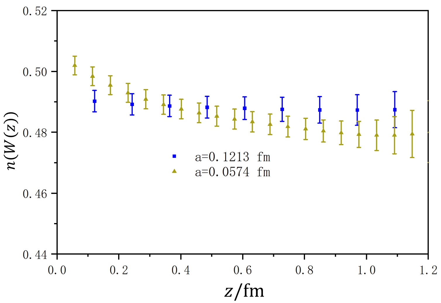


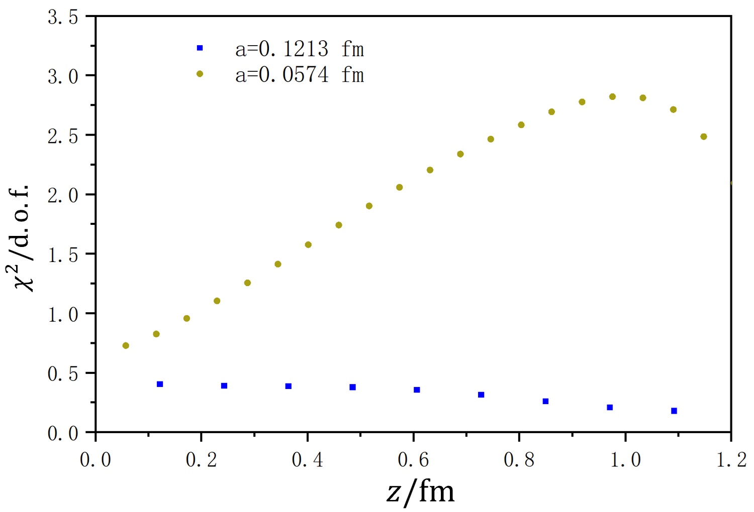
As shown in the upper and middle panels of Fig. 2, is approximately 0.5 and does not show a very strong dependence on and lattice spacing. Conversely, is much more sensitive to and lattice spacing. The lower panel indicates that the d.o.f. is sufficiently small. Thus, this empirical formula adequately captures the impact of imprecise gauge fixing in the Wilson line case.
The impact of imprecise gauge fixing increases as the Wilson line becomes longer, and it appears that this is primarily due to . Therefore, we fit and attempt to model it using a quadratic function as shown in the middle panel in Fig. 2. For a12m310, we obtain , , , and d.o.f.=0.06. For a06m310, the values are , , , and d.o.f.=0.51. This result suggests that will increase quadratically as the Wilson line lengthens, allowing us to use a quadratic function to forecast and assess the effect of imprecise gauge fixing. Interestingly, it appears that the coefficient is proportional to , and this term will become dominant when the Wilson line is sufficiently long.
The Wilson lines with gauge rotations and can be related by the following expression,
| (13) |
where and and just differ by the relative gauge rotations at both ends of the Wilson line. We can then use the correlation between the relative gauge rotation between the gauge fixing with different precision,
| (14) |
to gain insights into why depends on the gauge fixing precision. and are the gauge rotations with certain gauge fixing precision and .


As shown in the upper panel of Fig. 3, the correlation approaches 1 when the gauge fixing is precise enough, with . On the other hand, deviates from 1 for larger and approaches 0 in the limit of no gauge fixing. Such a deviation becomes more significant at large z, while suffering from loop-around effects when z is approximately L/2. These observations are consistent with the idea that gauge fixing creates a correlation between different spatial positions, which will be stronger with more precise gauge fixing.
At the same time, with a given but different lattice spacing also increases with , as shown in the lower panel of Fig. 3. This is also understandable since the correlation would depend on the distance in lattice units instead of physical units.
II.2 Straight Wilson line under gauge
We also extend our study of Wilson lines from Landau gauge with to the general covariant gauge. The gauge condition of gauge is defined as Giusti et al. (2001b); Zwanziger (1986); Giusti (1997),
| (15) |
where random matrix on each lattice site of each configuration belonging to the group are sampled according to the weight . Note that the Landau gauge is recovered when at every . The precision of gauge fixing for the gauge is defined as,
| (16) |
We use this expression in gauge instead of in this case.


As we did for Landau gauge, we plot the ratio
| (17) |
of the traces of Wilson lines defined in Eq. (11) for different precision of gauge fixing, with since it is very hard to reach higher precision here. The numerical gauge fixing requires more iteration steps to converge when becomes larger. Additionally, some configurations can not converge within 100,000 iterations if the required precision is too high, particularly for large .
As shown in the upper panel of Fig. 4, it seems that the impact of imprecise gauge fixing becomes slightly smaller as increases. The middle and lower panels show that the effects of lower required precision are larger on finer lattices, at longer distances and for lower average precision. This observation is consistent with our findings in Landau gauge.
II.3 Staple shaped Wilson line under Landau gauge
Staple shaped Wilson lines are also widely used gauge dependent measurement. For example, a quasi TMD-PDF operator Ji et al. (2020) contains a staple shaped Wilson line. Staple shaped Wilson lines are defined as,
| (18) |
where and are the separations between the two endpoints of the staple shaped Wilson line along the transverse direction and longitudinal direction , respectively. Straight Wilson lines are recovered when . The trace is denoted as as in the Wilson line case.


When considering the staple shaped Wilson lines and its trace for different gauge fixing, the only difference lies in the gauge transformation on the two endpoints. When and remain unchanged, the endpoints are fixed, but still has an influence on the impact of imprecise gauge fixing, as depicted in Fig. 5. When becomes longer, the impact of imprecise gauge fixing is enhanced as shown in the upper panel of Fig. 5. Furthermore, longer and smaller lattice spacing make this phenomena more pronounced, as shown in the middle and lower panels of Fig. 5. As the gauge fixing precision dependence is not very sensitive on , we will not delve into the discussion of the staple-shaped Wilson line in the gauge.
III Quasi PDF
A quasi-PDF operator is a quark bilinear operator with a Wilson line,
| (19) |
Its renormalized nucleon matrix element is connected to PDFs through factorization theorems Ji (2013, 2014); Ma and Qiu (2018a, b); Izubuchi et al. (2018). Its hadron matrix element is
| (20) |
The UV divergence is independent of the hadron state, as shown in Refs. Zhang et al. (2021); Huo et al. (2021). In the following we will concentrate on the pion matrix element of the quasi PDF operator at different lattice spacing as an illustrative example. The pion matrix element can be extracted from the following ratio
| (21) |
where is the mass gap between the pion and its first excited state which is aournd 1 GeV. One-step HYP smearing is applied to the Wilson lines to enhance the signal to noise ratio (SNR). The source/sink setup and also the ground state matrix element extraction are similar to that in Refs. Zhang et al. (2021); Huo et al. (2021); Zhang et al. (2022).
III.1 Quasi PDF renormalized using the Wilson line
In lattice regularization, one encounters a linear divergence of the quasi PDF operator defined in Eq. (19). To ensure the existence of a finite continuum limit, it is necessary to remove this linear divergence. Studies in the continuum Ji and Zhang (2015); Ji et al. (2018); Ishikawa et al. (2017); Green et al. (2018) suggest that the quasi-PDF operator is multiplicatively renormalizable, and the linear divergence just comes from the Wilson line. We plot the ratio of the pion matrix element and the trace of the Wilson line to see whether there is a residual linear divergence on the lattice.
The central value of the pion matrix element with Coulomb wall source shows negligible dependence on the precision of Coulomb gauge fixing, as demonstrated in the appendix. So we will concentrate on the precision of Landau gauge fixing used for the Wilson line rather than Coulomb gauge fixing used for the pion matrix element with wall source.


As shown in Fig. 6, the results at differ for different lattice spacings. The discrepancy increases for finer lattices and longer Wilson lines. When the precision of gauge fixing is increased, such as to , the results show convergence. Moreover, for , the results from different lattice spacings are consistent within uncertainty even for the finest lattice and at long distance, indicating the complete elimination of the linear divergence. Although at short distance, the results for , and are very close to each other, the impact of imprecise gauge fixing becomes significant at long distance, especially for smaller lattice spacing. This is due to the unphysical contribution caused by imprecise gauge fixing of Wilson lines, as mentioned previously.
Since the ratio has removed the linear divergence properly, one can do the perturbative calculation of to match the hadron matrix element to the scheme. First define a ”subtracted” quasi PDF renormalized in the short-distance ratio (SDR) scheme which divide the quasi PDF by the Wilson line and normalized with a pion matrix element in the rest frame at a short distance ,
| (22) |
Then can be matched to the scheme using the perturbative calculation of , and the on-shell which is independent of ,
| (23) |
where
| (24) |
Note that since the long Wilson line does contain non-perturbative physics at large-, the above approach will introduce some unknown non-perturbative effects. The comparison with other renormalization schemes can be found in the following subsection.
III.2 Quasi PDF renormalized in RI/MOM scheme and self renormalization
In RI/MOM renormalization, we need to calculate gauge dependent quark matrix elements to renormalize hadron matrix elements to get results free of any residual divergences. The definition of the renormalization constant is (e.g., Liu et al. (2020)),
| (25) |
where is the off-shell quark state with external momentum , and we have assumed a lattice regularization and included the dependence in the matrix elements. The setup in the calculation of quark matrix elements is the same as that in Ref. Zhang et al. (2021), except for the precision of gauge fixing. is defined from the hadron matrix element of a local vector current,
| (26) |
When the Landau gauge fixed volume source Chen et al. (2018) is used in the calculation, the statistical uncertainty is suppressed by a factor compared to the point source case. Note that the definition used here is exactly the same as from the quark propagator in dimensional regularization Gracey (2003), but the discretization effect is much smaller than that for in lattice regularization as shown in Ref. Chang et al. (2021).
We multiply the pion matrix element with to obtain the non-perturbatively renormalized and normalized matrix element at a given RI/MOM scale ,
| (27) |
Since the quasi-PDF operator is multiplicatively renormalizable and the linear divergence just comes from the Wilson line and is independent of the external quark or hadron state, RI/MOM renormalization Martinelli et al. (1995) is believed to be a good candidate to remove the linear divergence Constantinou and Panagopoulos (2017); Green et al. (2018); Chen et al. (2018); Stewart and Zhao (2018); Alexandrou et al. (2017, 2020); Lin et al. (2020).


If the linear divergence just comes from the Wilson line and is independent of the external quark or hadron state, then RI/MOM renormalization Martinelli et al. (1995) can be a good candidate to remove the linear divergence Constantinou and Panagopoulos (2017); Green et al. (2018); Chen et al. (2018); Stewart and Zhao (2018); Alexandrou et al. (2017, 2020); Lin et al. (2020). But similar to Wilson line, the quasi PDF quark matrix element in RI/MOM scheme is a non-local gauge dependent quantity, and thus it is also highly sensitive to the precision of Landau gauge fixing at long distance on fine lattices as shown in Fig. 7.
Compared to Fig. 1, we observe that the impact of imprecise gauge fixing on the quark matrix element is weaker than that on the Wilson line. This suggests that the quark external state mitigates the impact of imprecise gauge fixing. For example, the difference of the quark matrix elements at and on a06m310 at 1.2 fm is 0.021(0.012) whereas this difference is 0.032(0.003) for the Wilson line. Similarly, on a03m310, the difference is 0.06(0.03) and 0.116(0.09) for the quark matrix element and the Wilson line, respectively.


It is important to check whether the empirical formula defined in Eq. (12) can also describe the impact of imprecise gauge fixing on quark matrix elements. The fitted results are presented in Fig. 8. Here, is about 0.5 and increases for longer and smaller lattice spacing. The lower panel indicates that d.o.f. is not consistently small and can reach around 3 on a06m310. Nevertheless, we maintain that this empirical formula performs reasonably well. Ultimately, the precision of gauge fixing is unphysical, and there is some flexibility in its definition. Since is simply the trace of the Wilson line, it is more suitable for the Wilson line case than for the quark matrix element case when investigating the impact of imprecise gauge fixing. We believe that this empirical formula is sufficient to help us estimate the impact of imprecise gauge fixing for the quark matrix element. Additionally, we find that is negative on both a12m310 and a06m310, as , and d.o.f.=0.30 on a12m310, , and d.o.f.=0.36 on a06m310. The negative value of implies that defined in Eq. (III.2) will increase as the precision of Landau gauge fixing decreases, and that its impact can increase significantly at small lattice spacing.
We can perform a similar fit for using a quadratic function as shown in the middle panel in Fig. 8. On a12m310, we obtain , , , with d.o.f.=0.15. For a06m310, the values are , , , and d.o.f.=1.40. This result indicates that will grow quadratically as the Wilson line becomes longer. Consequently, we can employ a quadratic function to predict and estimate the impact of gauge fixing.


Thus the imprecise gauge fixing has an significant impact on quasi PDF in RI/MOM scheme. As shown in Fig. 9, the outcome at exhibits inconsistencies across various lattice spacings, with a more pronounced discrepancy observed for finer lattices. Furthermore, the discrepancy amplifies as the line lengthens. However, with an increased precision of gauge fixing, such as , the results behave better. Additionally, for , the results for different lattice spacings agree within the uncertainties, even on the finest lattice and at long distances, indicating the complete elimination of the linear divergence. If the precision is not high enough, the divergent behavior may be mistaken for residual linear divergence, as what we did in Ref. Zhang et al. (2021).
Even though the RI/MOM renormalization with precise enough gauge fixing can eliminate the linear divergence, the non-perturbative effect at large remains. Thus one can also extract divergent renormalization factors of quasi-PDF by parameterizing the results in the rest frame on the lattice, which is called self renormalization Huo et al. (2021).
The fit strategy used in Ref. Huo et al. (2021) can be improved into a joint fit of the results at different lattice spacing and Wilson line length :
| (28) |
where the linear divergence factor , the effective QCD scale , the discretization effect coefficient , the renormalon factor , the overall correction coefficient , and the renormalized matrix element are the parameters to be fitted, and represents the quasi-PDF in the scheme at 1-loop level.
It is important for and to be sufficiently large to mitigate discretization effects, yet small enough to ensure the validity of perturbative theory. Additionally, should not be excessively small. In this work, we choose and , and interpolate the data at different lattice spacing with intervals of 0.03 fm since both and depend on .
Based on this strategy, the renormalized quasi-PDF in the rest frame in the scheme will be
| (29) |

The conversion factor between RI/MOM and at 1-loop level can be found in Ref. Constantinou and Panagopoulos (2017). As shown in Fig. 10, the results using the self renormalization, the intermediate RI/MOM or SDR schemes are consistent with each other and close to the perturbative result at short distance, but they deviate from each other at long distance due to the non-perturbative effect from the intrinsic scale introduced in RI/MOM and SDR schemes.
III.3 Coulomb gauge quasi PDF
The Coulomb gauge quasi PDF Gao et al. (2023) (CG qPDF) operator is
| (30) |
At next-to leading order (NLO), its LaMET matching to PDFs has been demonstrated in Ref. Gao et al. (2023). This operator is non-local and its hadron matrix element is gauge dependent because the quark fields in the operator are non-local and not linked by Wilson lines. If it is the free of the linear divergence, the residual log divergence can be removed by a short distance matrix element,
| (31) |
The hadron matrix element is non-local and gauge dependent, similar to the quark matrix elements of quasi PDFs and quasi TMD-PDFs. Therefore, it is expected to be sensitive to the precision of gauge fixing.


We performed calculations on the MILC ensembles a06m310 and a045m310, with lattice spacings close to 0.06 fm and 0.04 fm, respectively, as used in Ref. Gao et al. (2023). As shown in Fig. 11, the results are not consistent with each other when the precision of Coulomb gauge fixing is set to . If we improve the precision to , the results are more consistent. This suggests absence of linear divergences or residual logarithm divergences in normalized CG qPDFs.
IV Quasi TMD-PDF
As a natural generalization of the collinear PDFs, the transverse-momentum-dependent (TMD) PDFs provide a useful description of the transverse structure of hadrons. In LaMET, the calculation of TMD-PDFs starts from the unsubtracted quasi TMD-PDF Ji et al. (2020); Ebert et al. (2019); Ji et al. (2021). The quasi TMD-PDF operator is a quark bilinear operator with staple-shaped Wilson line,
| (32) |
should be large enough to approximate the infinitely long Wilson line in the continuum. Similar as for the quasi PDF case, we focus on the pion matrix element and the unpolarized case (). Details in the RI/MOM scheme can be found in Ref. Zhang et al. (2022). Similar to quasi PDFs, quasi TMD-PDF hadron matrix elements are denoted as , and renormalized matrix elements in the RI/MOM scheme are denoted as .


As shown in the upper panel of Fig. 12, the results from different all saturate to a plateau. This indicates that the pinch pole singularity has been eliminated by the quark matrix element on the lattice. For a well-defined quasi-TMD operator, should be larger than the spatial parton distribution and independent of after proper subtraction. However, the statistical uncertainty will be larger at longer . In practice, we can choose a proper to balance the statistical uncertainty and systematic uncertainty, as we did in Ref. Zhang et al. (2022).
As shown in the lower panel of Fig. 12, the results at from different lattice spacings exhibit consistency, similar to the behavior observed in the quasi PDF case with . This suggests that the elimination of linear divergence, logarithmic divergence and cusp divergence have been achieved, and the precision is adequate in this case. If the precision of Landau gauge fixing is as as in Ref. Zhang et al. (2022), convergent behavior cannot be observed in the RI/MOM scheme.
The conversion factor between RI/MOM and can be found in Ref. Constantinou et al. (2019); Ebert et al. (2020). The reason why their perturbative results do not converge is that there is a pinch pole singularity in quasi TMD-PDFs. As increases, the conversion factor does not converge, resulting in a huge value. One method that can be used to remove the pinch pole singularity Ji et al. (2021) is dividing quasi TMD-PDF matrix elements by the square root of a rectangular Wilson loop. The calculation on a lattice will not be affected because the contributions of a Wilson loop in the quark matrix element and the hadron matrix element cancel each other out. This procedure has also been mentioned in other work, such as Ref. Alexandrou et al. (2023); Spanoudes et al. (2024). What we really need to do is adding a Wilson loop term to the conversion factor.

On the other hand, Ref. Zhang et al. (2022) proposed the short distance ratio scheme which is gauge invariant and can also be converted to the scheme through perturbative matching. To get rid of the pinch pole singularity and the linear divergence from the Wilson link self-energy, a more convenient “subtracted” quasi-TMD-PDF is then formed Ji et al. (2020),
| (33) |
We write the fully renormalized quasi-TMD-PDF as
| (34) |
where we also chosen the pion matrix element in the denominator (denoted by the subscript ) likes the quasi-PDF case. For simplicity, we have also chosen . The singular dependence on on the r.h.s. of Eq. (34) has been cancelled, leaving a dependence on the perturbative short scale . To perform the renormalization, the pion matrix element needs to be calculated non-perturbatively on the lattice. In order to match the renormalized quasi-TMD-PDF to the standard TMD-PDF, we also need the perturbative results of the above matrix elements, for which we can choose on-shell quark external states. The numerator of the r.h.s. of Eq. (34) has been calculated previously in dimensional regularization (DR) and scheme in Ref. Ebert et al. (2019), whereas the denominator is independent of and reads
| (35) |
With this, we can also convert the SDR result to the scheme via
| (36) |
where the dependence cancels.
As shown in Fig. 13, both results are consistent with each other and are close to the perturbative result at short distance, and they deviate from each other at long distance due to the non-perturbative effects from the intrinsic scales and/or introduced in RI/MOM scheme.
V Summary
We have investigated the gauge fixing precision dependence for several measurements, using 5 lattice spacings, in Landau gauge, Coulomb gauge and gauge. Our results indicate that the linear divergences in quasi PDF operators and quasi TMD-PDFs all comes from Wilson lines, and are independent of the external state when the gauge fixing is precise enough. There is also no linear divergence in Coulomb gauge quasi PDFs renormalized by short distance matrix elements.
Thus, we verified that self-renormalization, which fits the hadron matrix elements at different lattice spacings, RI/MOM renormalization, which uses the quark matrix element and precise enough Landau gauge fixing, and the short-distance renormalization, which divides by the corresponding Wilson line or square root of the Wilson loop, can fully eliminate the UV divergence of the quasi-PDF and quasi-TMD matrix elements, and make the renormalized ones finite in the continuum limit. Obviously the combinations of RI/MOM and SDR schemes (e.g. the short distance RI/MOM scheme Alexandrou et al. (2023)) should also have a finite continuum limit.
At the same time, even though all the approaches are consistent with the perturbative results at short distances up to the discretization error, they can be significantly different at long distances due to introduction of spurious infrared physics in RI/MOM and similar schemes. Therefore, the proper removal of the non-perturbative effects, such as self-renormalization, should be crucial to obtain reliable matrix elements at long distances.
When the gauge fixing precision is restricted, the dependence of the results on the gauge fixing residual can be roughly approximated by , where grows quadratically with the Wilson line length for both Wilson lines and quark matrix elements. Since the accurate gauge fixing with can be extremely costly on large lattices, this empirical formula can aid in estimating the systematic uncertainty stemming from imprecise gauge fixing. For example, if we requires the systematic uncertainty from the imprecise gauge fixing to be 1% at fm and fm , then the should be around .
Acknowledgement
We thank the MILC collaborations for providing us their gauge configurations, and Xiang Gao, Xiangyu Jiang, Peter Petreczky, and Yong Zhao for useful information and discussions. The calculations were performed using the Chroma software suite Edwards and Joo (2005) with QUDA Clark et al. (2010); Babich et al. (2011); Clark et al. (2016) through HIP programming model Bi et al. (2020). The numerical calculation were carried out on the ORISE Supercomputer, and HPC Cluster of ITP-CAS. This work is supported in part by NSFC grants No. 12293060, 12293062, 12293065 and 12047503, the science and education integration young faculty project of University of Chinese Academy of Sciences, the Strategic Priority Research Program of Chinese Academy of Sciences, Grant No. XDB34030303 and YSBR-101, and also a NSFC-DFG joint grant under Grant No. 12061131006 and SCHA 458/22.
References
- Martinelli et al. (1995) G. Martinelli, C. Pittori, C. T. Sachrajda, M. Testa, and A. Vladikas, Nucl. Phys. B445, 81 (1995), arXiv:hep-lat/9411010 [hep-lat] .
- Mandula (1999) J. E. Mandula, Phys. Rept. 315, 273 (1999), arXiv:hep-lat/9907020 .
- Wilson (1974) K. G. Wilson, Phys. Rev. D 10, 2445 (1974).
- Mandula and Ogilvie (1987) J. E. Mandula and M. Ogilvie, Phys. Lett. B 185, 127 (1987).
- Katz et al. (1988) G. Katz, G. Batrouni, C. Davies, A. S. Kronfeld, P. Lepage, P. Rossi, B. Svetitsky, and K. Wilson, Phys. Rev. D 37, 1589 (1988).
- Giusti et al. (2001a) L. Giusti, M. L. Paciello, C. Parrinello, S. Petrarca, and B. Taglienti, Int. J. Mod. Phys. A 16, 3487 (2001a), arXiv:hep-lat/0104012 .
- Lytle et al. (2018) A. T. Lytle, C. T. H. Davies, D. Hatton, G. P. Lepage, and C. Sturm (HPQCD), Phys. Rev. D 98, 014513 (2018), arXiv:1805.06225 [hep-lat] .
- Ji (2013) X. Ji, Phys. Rev. Lett. 110, 262002 (2013), arXiv:1305.1539 [hep-ph] .
- Ji et al. (2021) X. Ji, Y.-S. Liu, Y. Liu, J.-H. Zhang, and Y. Zhao, Rev. Mod. Phys. 93, 035005 (2021), arXiv:2004.03543 [hep-ph] .
- Gao et al. (2023) X. Gao, W.-Y. Liu, and Y. Zhao, (2023), arXiv:2306.14960 [hep-ph] .
- Hart et al. (2009) A. Hart, G. M. von Hippel, and R. R. Horgan (HPQCD), Phys. Rev. D 79, 074008 (2009), arXiv:0812.0503 [hep-lat] .
- Bazavov et al. (2013) A. Bazavov et al. (MILC), Phys. Rev. D87, 054505 (2013), arXiv:1212.4768 [hep-lat] .
- Edwards and Joo (2005) R. G. Edwards and B. Joo (SciDAC, LHPC, UKQCD), Lattice field theory. Proceedings, 22nd International Symposium, Lattice 2004, Batavia, USA, June 21-26, 2004, Nucl. Phys. Proc. Suppl. 140, 832 (2005), [,832(2004)], arXiv:hep-lat/0409003 [hep-lat] .
- Giusti et al. (2001b) L. Giusti, M. L. Paciello, S. Petrarca, and B. Taglienti, Phys. Rev. D 63, 014501 (2001b), arXiv:hep-lat/9911038 .
- Zwanziger (1986) D. Zwanziger, NATO Sci. Ser. B 141, 345 (1986).
- Giusti (1997) L. Giusti, Nucl. Phys. B 498, 331 (1997), arXiv:hep-lat/9605032 .
- Ji et al. (2020) X. Ji, Y. Liu, and Y.-S. Liu, Nucl. Phys. B 955, 115054 (2020), arXiv:1910.11415 [hep-ph] .
- Ji (2014) X. Ji, Sci. China Phys. Mech. Astron. 57, 1407 (2014), arXiv:1404.6680 [hep-ph] .
- Ma and Qiu (2018a) Y.-Q. Ma and J.-W. Qiu, Phys. Rev. D98, 074021 (2018a), arXiv:1404.6860 [hep-ph] .
- Ma and Qiu (2018b) Y.-Q. Ma and J.-W. Qiu, Phys. Rev. Lett. 120, 022003 (2018b), arXiv:1709.03018 [hep-ph] .
- Izubuchi et al. (2018) T. Izubuchi, X. Ji, L. Jin, I. W. Stewart, and Y. Zhao, Phys. Rev. D98, 056004 (2018), arXiv:1801.03917 [hep-ph] .
- Zhang et al. (2021) K. Zhang, Y.-Y. Li, Y.-K. Huo, A. Schäfer, P. Sun, and Y.-B. Yang (QCD), Phys. Rev. D 104, 074501 (2021), arXiv:2012.05448 [hep-lat] .
- Huo et al. (2021) Y.-K. Huo et al. (Lattice Parton Collaboration (LPC)), Nucl. Phys. B 969, 115443 (2021), arXiv:2103.02965 [hep-lat] .
- Zhang et al. (2022) K. Zhang, X. Ji, Y.-B. Yang, F. Yao, and J.-H. Zhang ([Lattice Parton Collaboration (LPC)]), Phys. Rev. Lett. 129, 082002 (2022), arXiv:2205.13402 [hep-lat] .
- Ji and Zhang (2015) X. Ji and J.-H. Zhang, Phys. Rev. D92, 034006 (2015), arXiv:1505.07699 [hep-ph] .
- Ji et al. (2018) X. Ji, J.-H. Zhang, and Y. Zhao, Phys. Rev. Lett. 120, 112001 (2018), arXiv:1706.08962 [hep-ph] .
- Ishikawa et al. (2017) T. Ishikawa, Y.-Q. Ma, J.-W. Qiu, and S. Yoshida, Phys. Rev. D96, 094019 (2017), arXiv:1707.03107 [hep-ph] .
- Green et al. (2018) J. Green, K. Jansen, and F. Steffens, Phys. Rev. Lett. 121, 022004 (2018), arXiv:1707.07152 [hep-lat] .
- Liu et al. (2020) Y.-S. Liu et al. (Lattice Parton), Phys. Rev. D101, 034020 (2020), arXiv:1807.06566 [hep-lat] .
- Chen et al. (2018) J.-W. Chen, T. Ishikawa, L. Jin, H.-W. Lin, Y.-B. Yang, J.-H. Zhang, and Y. Zhao, Phys. Rev. D97, 014505 (2018), arXiv:1706.01295 [hep-lat] .
- Gracey (2003) J. A. Gracey, Nucl. Phys. B662, 247 (2003), arXiv:hep-ph/0304113 [hep-ph] .
- Chang et al. (2021) L. Chang, Y.-B. Liu, K. Raya, J. Rodríguez-Quintero, and Y.-B. Yang, (2021), arXiv:2105.06596 [hep-lat] .
- Constantinou and Panagopoulos (2017) M. Constantinou and H. Panagopoulos, Phys. Rev. D 96, 054506 (2017), arXiv:1705.11193 [hep-lat] .
- Stewart and Zhao (2018) I. W. Stewart and Y. Zhao, Phys. Rev. D97, 054512 (2018), arXiv:1709.04933 [hep-ph] .
- Alexandrou et al. (2017) C. Alexandrou, K. Cichy, M. Constantinou, K. Hadjiyiannakou, K. Jansen, H. Panagopoulos, and F. Steffens, Nucl. Phys. B923, 394 (2017), arXiv:1706.00265 [hep-lat] .
- Alexandrou et al. (2020) C. Alexandrou, K. Cichy, M. Constantinou, J. R. Green, K. Hadjiyiannakou, K. Jansen, F. Manigrasso, A. Scapellato, and F. Steffens, (2020), arXiv:2011.00964 [hep-lat] .
- Lin et al. (2020) H.-W. Lin, J.-W. Chen, and R. Zhang, (2020), arXiv:2011.14971 [hep-lat] .
- Ebert et al. (2019) M. A. Ebert, I. W. Stewart, and Y. Zhao, JHEP 09, 037 (2019), arXiv:1901.03685 [hep-ph] .
- Constantinou et al. (2019) M. Constantinou, H. Panagopoulos, and G. Spanoudes, Phys. Rev. D 99, 074508 (2019), arXiv:1901.03862 [hep-lat] .
- Ebert et al. (2020) M. A. Ebert, I. W. Stewart, and Y. Zhao, JHEP 03, 099 (2020), arXiv:1910.08569 [hep-ph] .
- Alexandrou et al. (2023) C. Alexandrou et al., Phys. Rev. D 108, 114503 (2023), arXiv:2305.11824 [hep-lat] .
- Spanoudes et al. (2024) G. Spanoudes, M. Constantinou, and H. Panagopoulos, (2024), arXiv:2401.01182 [hep-lat] .
- Clark et al. (2010) M. A. Clark, R. Babich, K. Barros, R. C. Brower, and C. Rebbi, Comput. Phys. Commun. 181, 1517 (2010), arXiv:0911.3191 [hep-lat] .
- Babich et al. (2011) R. Babich, M. A. Clark, B. Joo, G. Shi, R. C. Brower, and S. Gottlieb, in SC11 International Conference for High Performance Computing, Networking, Storage and Analysis Seattle, Washington, November 12-18, 2011 (2011) arXiv:1109.2935 [hep-lat] .
- Clark et al. (2016) M. A. Clark, B. Jo, A. Strelchenko, M. Cheng, A. Gambhir, and R. Brower, (2016), arXiv:1612.07873 [hep-lat] .
- Bi et al. (2020) Y.-J. Bi, Y. Xiao, M. Gong, W.-Y. Guo, P. Sun, S. Xu, and Y.-B. Yang, Proceedings, 37th International Symposium on Lattice Field Theory (Lattice 2019): Wuhan, China, June 16-22 2019, PoS LATTICE2019, 286 (2020), arXiv:2001.05706 [hep-lat] .
Appendix
V.1 The distribution of
The quantity , defined in Eq. (I) in Landau gauge, does not reach exactly zero at every lattice site due to imperfect gauge fixing. As illustrated in Fig. 14, the distribution is symmetrical and exhibits a long tail. It is important to note that the scale of the abscissa is smaller for higher precision. With a precision that is 100 times greater, the tail becomes approximately 10 times shorter. However, the tail does not display a strong dependence on lattice spacing. Additionally, we compute , as defined in Eq. (5), on the same configuration for comparison. The magnitude of is directly proportional to that of in the part of the ensemble that we are investigating.


V.2 Coulomb wall source
As our focus is solely on the UV divergence of the quasi-PDF operator, we utilize the pion in the rest frame as the external state to enhance the signal-to-noise ratio. Additionally, we have employed a Coulomb wall source to further improve the signal. It is well-known that wall source calculations include a gauge variation part, but with a sufficient number of configurations, the gauge variant part will vanish. And one finds that applying Coulomb gauge fixing improves the signal-to-noise ratio, but does not lead to an obvious systematic deviation. In this work, we aim to verify whether this holds true for non-local operator hadron matrix elements, and use the unpolarized quasi PDF as illustration.

As depicted in Fig. 15, the ratio remains close to one for various required precisions, as long as the Wilson lines are not excessively long. Consequently, we can conclude that the imprecise Coulomb gauge fixing in the wall source calculation in this study does not change the central values.