IKFlow: Generating Diverse Inverse Kinematics Solutions
Abstract
Inverse kinematics—finding joint poses that reach a given Cartesian-space end-effector pose—is a fundamental operation in robotics, since goals and waypoints are typically defined in Cartesian space, but robots must be controlled in joint space. However, existing inverse kinematics solvers return a single solution, in contrast, systems with more than 6 degrees of freedom support infinitely many such solutions, which can be useful in the presence of constraints, pose preferences, or obstacles. We introduce a method that uses a deep neural network to learn to generate a diverse set of samples from the solution space of such kinematic chains. The resulting samples can be generated quickly (2000 solutions in under 10ms) and accurately (to within 10 millimeters and 2 degrees of an exact solution) and can be rapidly refined by classical methods if necessary.
Index Terms:
Deep Learning Methods, KinematicsI Introduction
Inverse Kinematics (IK) maps a task-space Cartesian pose to a joint space configuration, which is a critically important operation for several reasons. For example, it is typically easier to define tasks in a specialized Cartesian coordinate frame that is easily interpretable by the robot’s operator—for example, specifying a curve to draw on a whiteboard is more easily done in the frame of the whiteboard than in the joint space of the robot. Similarly, it is beneficial to express a grasp pose in Cartesian space because it leaves the robot free to choose among a multitude of valid joint space poses. Of course, each Cartesian-space goal must be translated to a joint pose for the robot to control to; therefore, these scenarios are only possible with a fast IK solver.
Although there are several open source IK packages [3, 22, 6], their functionality is still incomplete. Analytical solvers like IKFast [8] and IKBT [22] are fast and return all the solutions for an arm, but cannot be applied to arms with more than 6 degrees of freedom (DOF). Numerical solvers can be applied to arms with any number of joints, but only return a single solution, if one is found at all. A solver that can provide many solutions for an arm with 7-DOF or greater, and do so quickly, would add significant functionality that would support more robust robot planning and control. More specifically, it allows for multiple joint solutions to be evaluated for any particular end effector pose. This is important for grasping in cluttered environments because there may be a large number of solutions that are in collision with an object. A large number of solutions is also important for the pathwise-Inverse Kinematics problem [18]. A complete mapping between joint space and task space enables planning to take place in the task space. IK can then be used to validate the task space plan with high confidence. Planning in the task space has a smaller dimension than joint space. This smaller dimension is useful for learning and sampling based approaches because fewer samples are required to cover the space with the same density.
An ideal 7+ DOF IK solver should return a set of solutions that covers the entire solution set. These samples should be near-exact solutions. Additionally, it should do so quickly. This allows the solver to serve as a primitive in the inner loop of higher-level decision-making algorithms. Of these three requirements, accuracy is the least important because verifying a sample using forward kinematics is very fast, and numerical IK solvers can be seeded with an approximate solution to rapidly refine to any desired accuracy.
We propose IKFlow, a new IK method that satisfies these requirements by training a neural network to output a diverse set of poses that approximately satisfy a given Cartesian goal pose. By viewing the problem as generative modeling problem over the solution space, we are able to exploit recent advances in Normalizing Flows [20]. Normalizing Flows are a generative modeling approach capable of modeling multi-modal distributions with nonlinear interactions between variables. We show, using several different kinematic models, that IKFlow can be trained—once off, per-robot—to rapidly generate hundreds to thousands of diverse approximate solutions; we also provide a practical open-source implementation of our approach.111https://sites.google.com/view/ikflow
II Background
II-A Inverse Kinematics (IK)
Inverse Kinematics defines the mapping from a robot’s operational space to its joint space:
where is the number of joints. The topology of the joint space is the n-dimensional torus, . The topology of is determined by the workspace of the robot, but we focus on the case where the end effector pose is in . If the robot has joint limits then the topology of the mapping changes:
where is the n-dimensional Euclidean space. This topological difference is important because it allows for many robots to be modeled by generic density estimators, instead of special purpose estimators built for tori [21].
II-A1 IK for 7+ DOF
When the degrees of freedom of the robot exceed the degrees of freedom of the operational space (i.e. the robot is kinematically redundant) there are infinitely many solutions. This occurs because the extra degree of freedom allows for a continuum of configurations that satisfy the desired Cartesian goal. Thus for a specific pose an IK solver should return a subset of joint space:
There are two current approaches for describing the solution space of 7+ DoF arms. The first category uses only a single point to describe the solution space, but returns quickly, on the order of millisecond. The second approach returns a more thorough set of solution points, by running the first approach with randomly sampled start states. In order to obtain a representative set of the solution space this approach requires extensive random sampling, and thus is significantly slower, on the order of seconds for thousands of solutions. The approach we detail in Section IV uses generative modeling to generate upwards of a thousand solutions in under milliseconds.
II-B Deep Generative Modeling
Generative modeling represents arbitrary distributions in such a way that they can be sampled. This is achieved by transforming known base distributions into target distributions. For example:
where is an arbitrary distribution and is a neural network. We additionally define the latent space as the space in which the base distribution lies - in our case , where is the dimension of the network. We draw samples from the arbitrary distribution by drawing samples from the base distribution and passing them through . There are several different generative modeling methods. In order to select an approach we used the following criteria. First, the diversity of samples returned is important to ensure that the full breadth of the solution space is returned. Second, the approach must be able to handle multi-modal data and nonlinear dependencies between variables in order to cover the solution space. Third, the method must be capable of handling conditional information, because the solution space is conditioned on the Cartesian goal. Fourth, the method must sample solutions quickly because IK is often used as a primitive by other procedures. Finally, the sampling procedure must produce samples with sufficient accuracy. Given these desired properties we propose to use a normalizing flow approach.
| Robot | DOF | Coupling Layer Width | Coupling Layers | Number of Parameters |
|---|---|---|---|---|
| ATLAS (2013) - Arm and Waist | 9 | 15 | 9 | |
| ATLAS (2013) - Arm | 6 | 15 | 12 | |
| Baxter | 7 | 15 | 16 | |
| Panda | 7 | 9 | 12 | |
| PR2 | 8 | 15 | 8 | |
| Robonaut 2 - Arm and Waist | 8 | 15 | 12 | |
| Robonaut 2 - Arm | 7 | 15 | 12 | |
| Valkyrie - Whole Arm and Waist | 10 | 15 | 16 | |
| Valkyrie - Lower Arm | 4 | 15 | 9 | |
| Valkyrie - Whole Arm | 7 | 15 | 12 |
II-B1 Normalizing Flows
Normalizing Flows are a generative modeling approach that provides quick sampling, stable training and arbitrary data distribution fitting [16]. Normalizing flows are based on two components. The first component is a series of functions that are easy to invert. These easily invertible functions enable the same network to quickly estimate densities and produce samples. In the literature, this series of functions is commonly referred to as the coupling layers. Sampling is performed by passing a sample from the base distribution through each of the coupling layers:
| (1) |
where is the sample in the data space and is a sample from the base distribution. The second important component is the efficient calculation of the Jacobian’s determinant. This enables density estimation of a data point to be computed with the change of variables formula:
The change of variables formula allows a distribution over one set of variables to be described by another set of variables given the determinant of the Jacobian between the two variables. A normalizing flow uses this along with a simple prior distribution, —here a Normal distribution—to enable density estimation of the data distribution . To make the determinant of the Jacobian tractable, special coupling layers are used. The coupling layer used in IKFlow was developed by Kingma and Dhariwal [13]:
| (2) | ||||
| (3) | ||||
| (4) |
where is the input data to a layer, and is the output. affects the scaling of the layer, shifts the input of the layer, and . This layer is then inverted by:
An important property of the layers is that they can be inverted without inverting the function that produces and . , also known as the coefficient network, can therefore be arbitrarily complex. Further, by holding constant through the transformation, the Jacobian will have zeros in the upper diagonal, and thus the determinant will only be the product of the diagonals of the Jacobian.
II-B2 Conditional Normalizing Flows
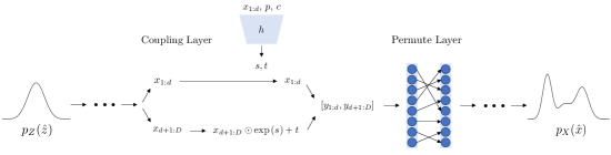
Conditional Normalizing Flows change the scaling and shifting of a coupling layer based on conditional information. The conditional information, , is passed as part of the input to the network which estimates and . Now is a function of both and . The invertibility of the coupling layer remains unaffected because the conditioning information is passed into which need not be inverted to invert the layer. Figure 2 provides a simple diagram of the architecture. While other methods have been proposed for conditioning normalizing flows (i.e. Ardizzone et al. [2]) this formulation reduces the number of hyperparameters that must be tuned, and has a simple Maximum Likelihood training loss:
| (5) |
For a more thorough review of Normalizing Flows see Papamakarios et al. [16].
II-B3 Maximum Mean Discrepancy (MMD)
Finally, a method for comparing distributions is necessary to evaluate the performance of a generative model. We use Maximum Mean Discrepancy (MMD) because of its strong theoretical properties and ease of implementation. Given two distributions, and , MMD computes the distance between the two distributions as the squared distance between the mean of the embeddings of the distributions.
Notably, the embeddings must be in a Reproducing Kernel Hilbert Space (RKHS). The capability of MMD to capture the distance between two distributions is dependent on the selection of a good embedding function . We selected the inverse multi-quadric kernel because of its long tails and previous use Ardizzone et al. [2]. A more detailed analysis of Maximum Mean Discrepancy is provided by Gretton et al. [10].
III Related Work
There have been a number of attempts to use neural networks for inverse kinematics [1, 5, 7, 19]. Most of these approaches do not solely implement the inverse kinematics function. For example, Csiszar et al. [5] incorporate the problem of calibrating the physical robot with its internal model. Almusawi et al. [1] learn the kinematics model in addition to performing Cartesian control. Demby’S et al. [7] create a neural network approach that focuses exclusively on the IK problem, but conclude that it is not a fruitful path because of large error.
The architectures used in the previous approaches are all fundamentally limited as they can only return a single solution for a particular input. However, IK is a one-to-many mapping, and access to additional solutions may prove useful for the control layer above IK. Ren and Ben-Tzvi [19] take a generative approach by using several different types of GANs, but the error of samples is worse than a fully connected network, with the best performing approach achieving 8cm of error. Ardizzone et al. [2] apply a similar deep generative approach to IKFlow but only to a small planar IK problem. We extend and refine their work in three key ways. First, we decrease the amount of error present in the solutions by adopting a conditional Invertible Neural Network. Second, we improve training stability by addressing a corner case related to the dimensionality of solution spaces. Third, we expand the coverage to include the entire physical workspace of the arm.
Kim and Perez [12] are the most similar point of comparison because they also use normalizing flows to solve inverse kinematics. IKFlow has several differences, the use of Conditional Normalizing Flows, the addition of training noise, and a sub-sampling procedure for the base distribution. These differences result in better performance for theoretical and practical reasons that are explained in the following section. Additionally, IKFlow doesn’t have a network that can calculate the forward kinematics, because the forward kinematics of a system are easy to calculate analytically. IKFlow’s single network can perform both inverse kinematics and density estimation, which are difficult to perform analytically but with reduced overall complexity. As a result of these differences, the accuracy achieved by IKFlow is x better in position, and x better in orientation, as measured with the Panda Arm and compared with Figure 3 in Kim and Perez [12].
IV IKFlow: Learned Inverse Kinematics
The first step to learning inverse kinematics is to treat the solution space as a distribution that has a uniform probability, which may have multiple intervals, and is conditioned on the desired pose. We model the solution distribution with Conditional Normalizing Flows because they are quicker than alternatives to sample, are stable when training, and are capable of representing the full solution space [14]. Additionally, they don’t face problems such as vanishing gradients or mode collapse which are common when training Generative Adversarial Networks (GANs), a different neural generative modeling approach [14].
There are three steps to applying Conditional Normalizing Flows to the inverse kinematics problem. First, a data set must be constructed. Second, we must select an architecture and parameters of the architecture. Third, we must design a loss function for minimizing the difference between samples from the generative model and the data distribution.
| Robot | DOF | MMD Score | Time (msec) | Average L2 Position Error (millimeters) | Avg Angular Error (degrees) |
|---|---|---|---|---|---|
| ATLAS (2013) - Arm and Waist | 9 | 0.03723 | 4.8 | 2.66 | 0.61 |
| ATLAS (2013) - Arm | 6 | 0.004828 | 6.4 | 1.19 | 0.28 |
| Baxter | 7 | 0.0331 | 8.29 | 4.5 | 1.19 |
| Panda | 7 | 0.0306 | 6.28 | 7.72 | 2.81 |
| PR2 | 8 | 0.2128 | 4.31 | 3.3 | 1.56 |
| Robonaut 2 - Arm and Waist | 8 | 0.03691 | 6.44 | 3.63 | 0.77 |
| Robonaut 2 - Arm | 7 | 0.0327 | 6.45 | 1.91 | 0.46 |
| Valkyrie - Whole Arm and Waist | 10 | 0.0361 | 8.55 | 3.49 | 0.74 |
| Valkyrie - Lower Arm | 4 | 1.508e-06 | 4.87 | 0.36 | 0.15 |
| Valkyrie - Whole Arm | 7 | 0.0292 | 6.45 | 1.64 | 0.38 |
IV-A Data Generation
One advantage of the inverse kinematics problem is the relative ease with which data can be generated. All serial kinematic chains have known forward kinematics that can be used to generate training data. Data is generated by uniformly sampling from the interval defined by the joint limits. The joint samples are then fed through a forward kinematics function to obtain the corresponding Cartesian pose. The Cartesian pose becomes the conditional input to the network and the joint data is used as the target distribution. More sophisticated sampling methods could be used to account for effects at joint limits and for self-collisions, but we were able to obtain satisfactory performance without them and thus leave this investigation for future work.
IV-B Normalizing Flow Architecture
The fundamental architecture of the network is defined by the use of normalizing flows, and was detailed in equations 1-4. The remaining design choices include the selection of a base distribution, selecting the number of coupling layers, the width of each coupling layer, and specification of the coefficient network.
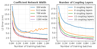
The base distribution affects the complexity of the density estimation and the sampling speed. We chose the Normal distribution because it simplifies the calculation of the Maximum Likelihood Loss function and is quick to sample. The remaining choices for the architecture affect the capability of the network to fit a target distribution. The width of each coupling layer must be at least as large as the degrees of freedom; if it is larger than the DOF it allows for multi-modal distributions to be more easily modeled. The number of coupling layers required depends on the interactions of joints with each other. The more complex the inter-joint relationship, the more coupling layers are required, as more layers allow for more interaction between joints because of the permutation layers. The number of coupling layers and the width of each can be found automatically by performing a hyper parameter sweep over a reasonable range (i.e. [, ] and [, ]). Finally, the coefficient network must be expressive enough to capture dependencies between the conditional information (i.e. the goal pose) and a subset of the layer values. Table I details the variable parameters (selected by hyperparameter search) for each kinematic chain that we test. An analysis was performed to demonstrate the impact of the number of coupling layers and the width of the coefficient function networks on the average Positional error of a network Figure 4. This demonstrates that the error of a network decreases with increased size up to a point, at which point increasing the network size does not improve performance.
IV-C Loss Functions
The Maximum Likelihood loss detailed in equation 5 is theoretically the only loss function necessary for achieving high performance. However, for several of the kinematic chains tested, training diverged when trained with the Maximum Likelihood loss. The cause of this divergence was a mismatch between the dimension of the solution manifolds and the base distribution.
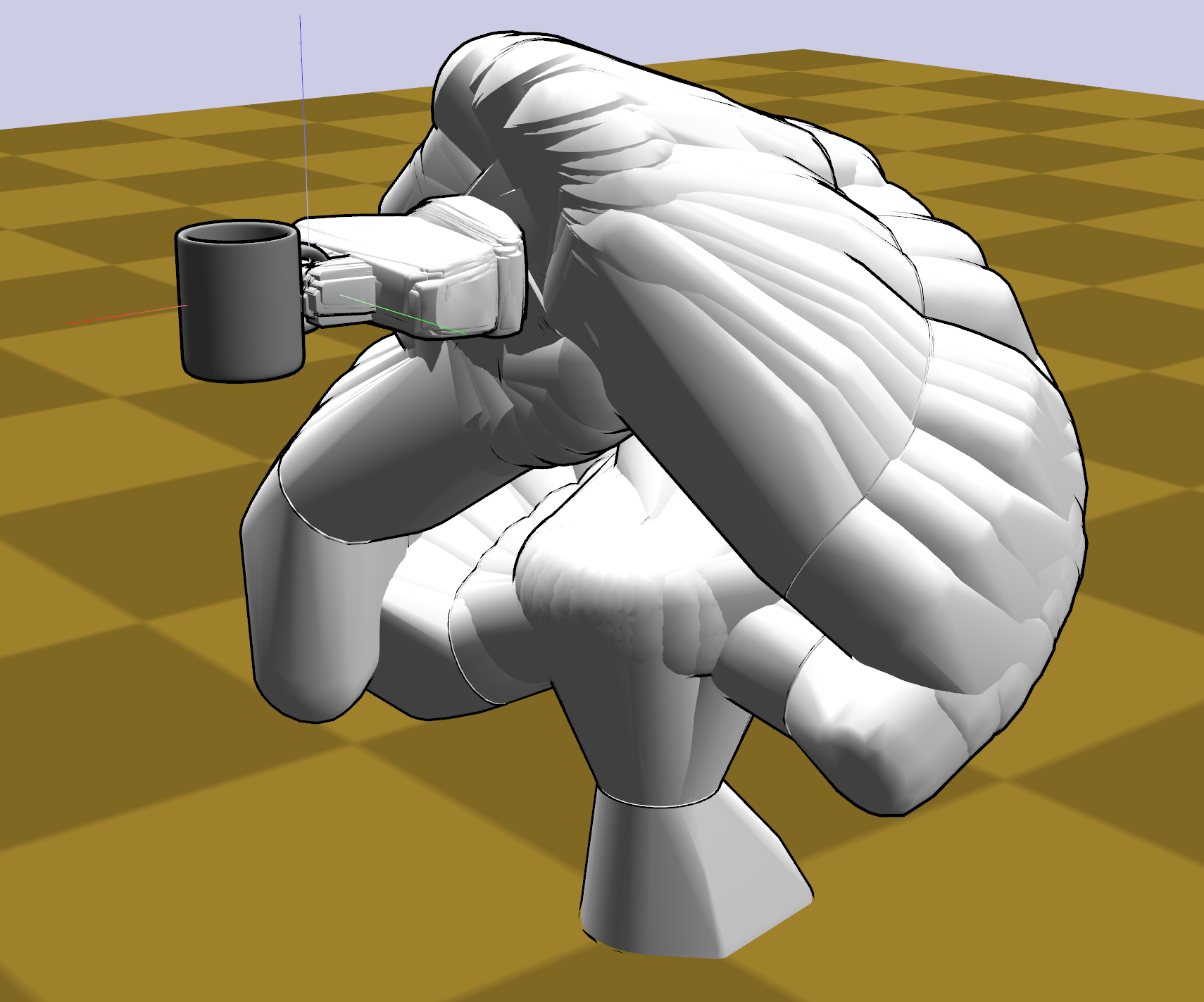
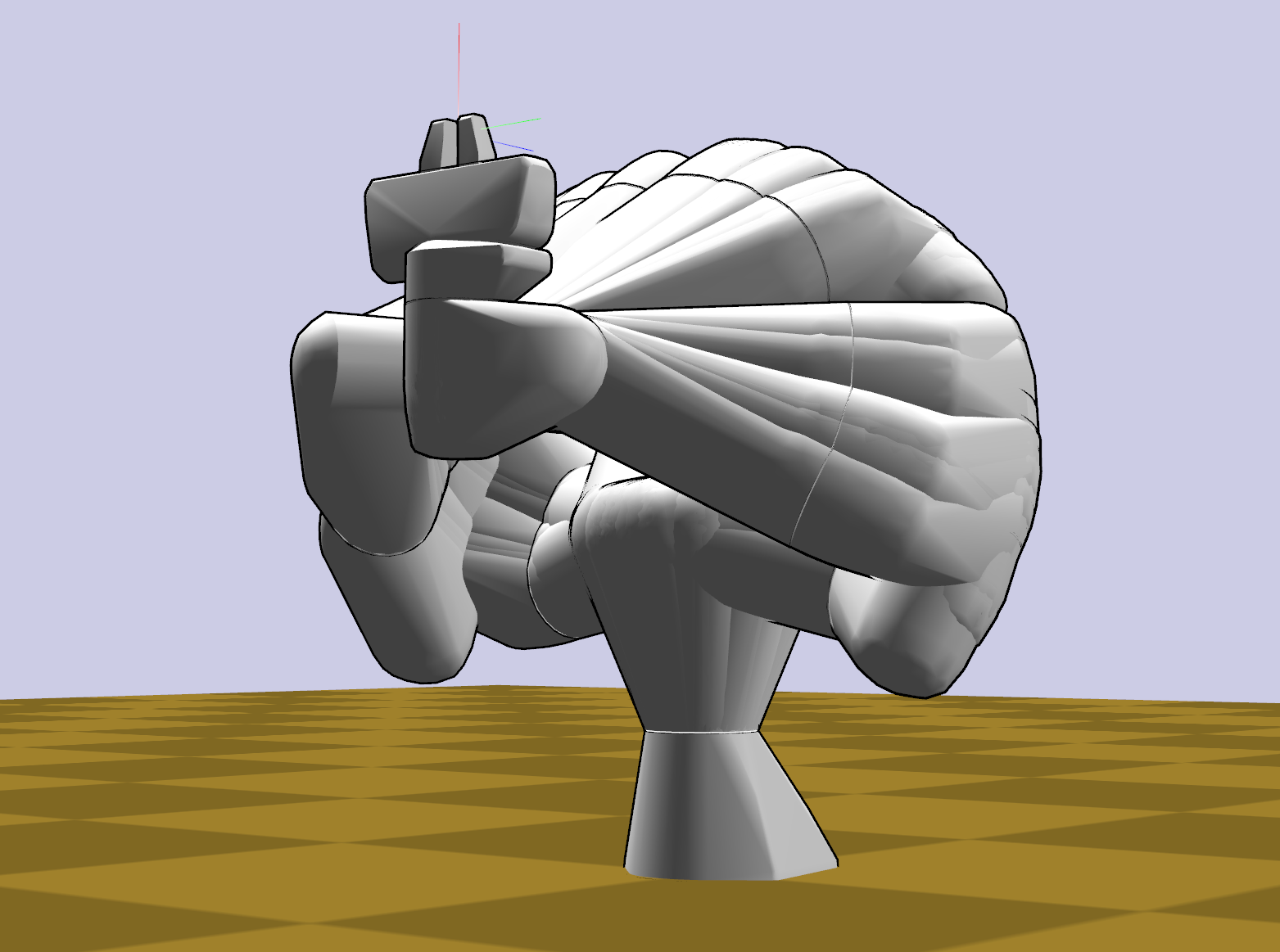
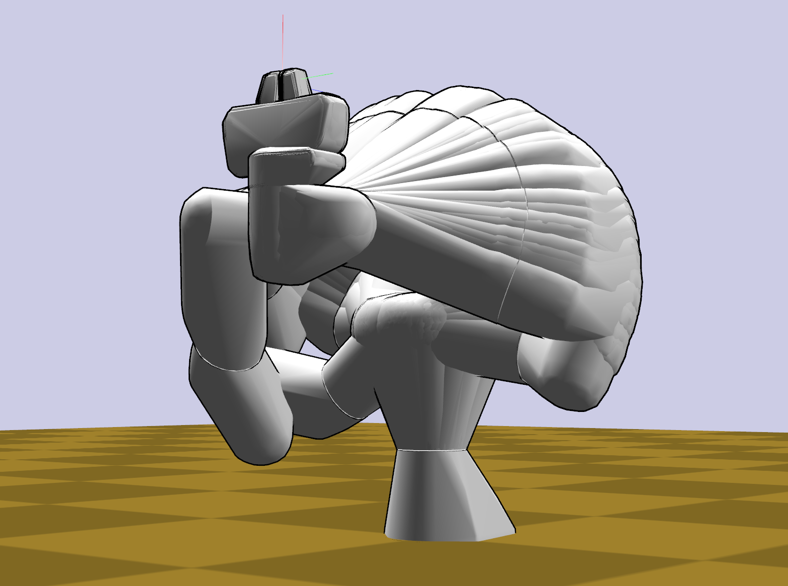
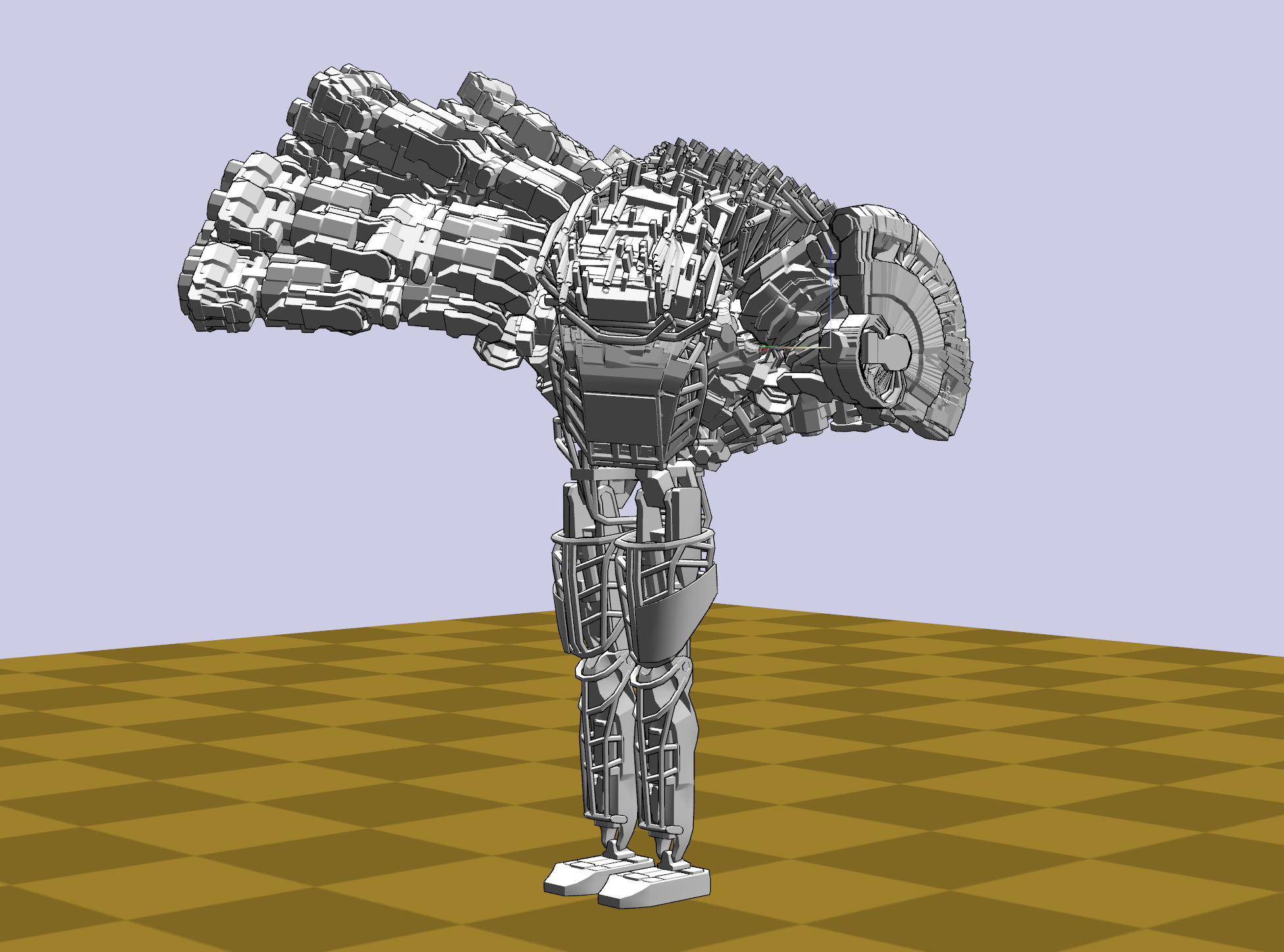
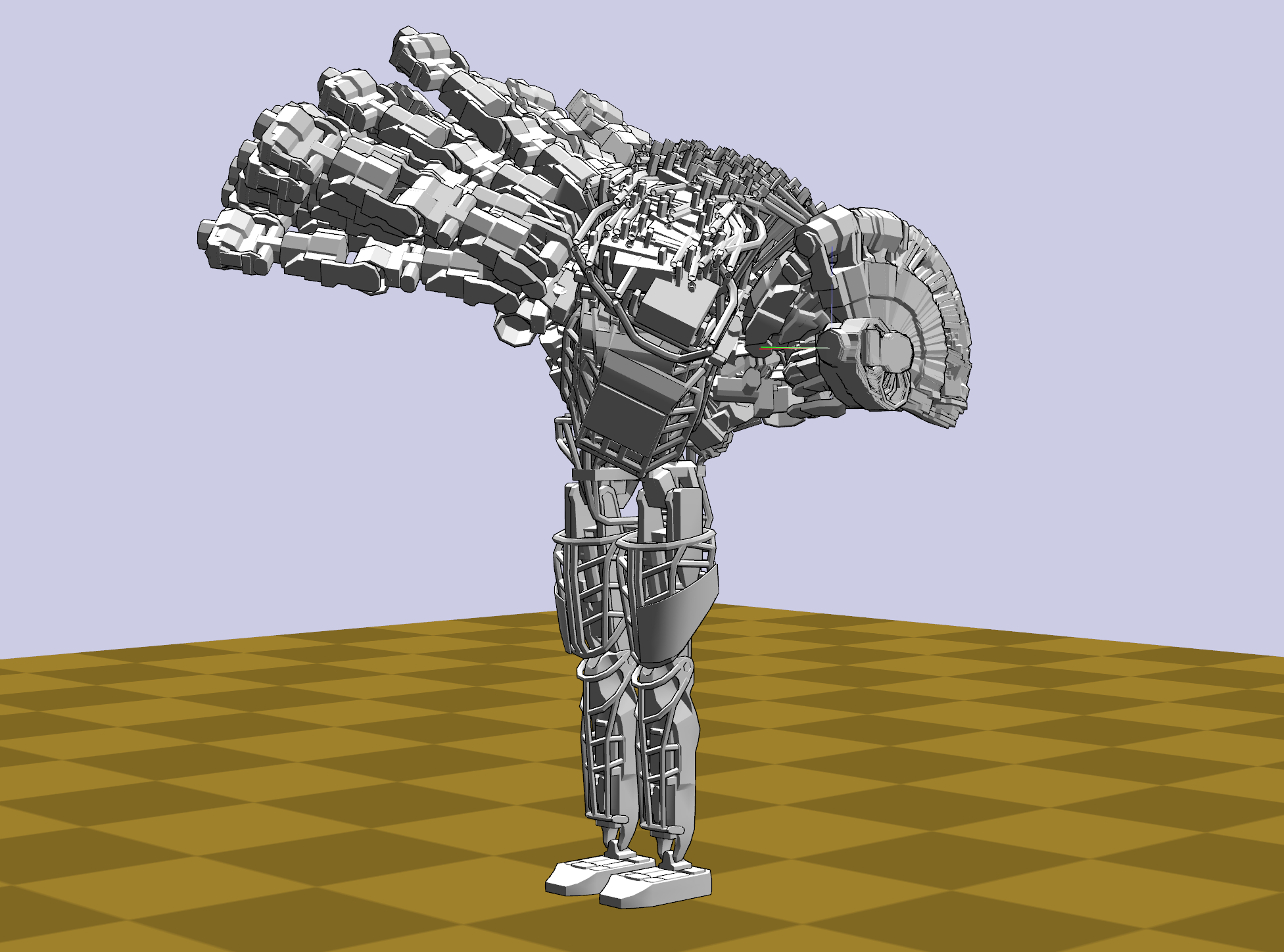
IV-C1 Solution Sub-manifolds
In Figure 3(a) the last joint of the arm appears in only one position. This implies that the solution space of that particular pose is not the same dimension as the joint space, because only 6 of the 7 joints in the arm can vary. This is not a unique situation, but occurs throughout the configuration space as some Cartesian poses can only be reached by fixing one of the joints at a specific configuration, for example at one of its limits. This is problematic because the normalizing flow approach does not perform well on distributions that are lower dimension than the base distribution. Specifically, the change of variables equation (II-B1) does not hold if the base distribution and the target distribution are not the same dimension. One way to ensure the target distribution and the base distribution are the same dimension is to add noise that is the full dimension [11]. If the magnitude of the added noise is passed in as a conditional variable, its effect can be removed at test time by setting that piece of the conditional to 0:
where and are drawn every training iteration, and added to the training data. The resulting loss function is:
| (6) |
where is the desired Cartesian pose.
IV-D Base Distribution Sub-sampling
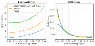
One down side of using the Normal distribution for the base distribution is the tails of the distribution. At evaluation time a point sampled from the tail of the Normal distribution is likely to produce a solution that has high error because the loss function encourages known solutions to be closer to the mean of the distribution. In order to reduce the impact of the tails the base distribution is sub-sampled at test time. This reduces the likelihood of a point from the tail of a distribution, however this encourages less diverse solutions. This trade off is demonstrated by Figure 7. Thus the scaling of the base distribution should be treated as a tuning parameter for the particular application of IKFlow.
V Experiments
The models were built with the FrEIA framework [2] and trained with PyTorch [17]. Additional details about the network architectures and training parameters can be found in the appendix. Once trained the model was evaluated on the three desired quantities: speed, accuracy, and solution space coverage.
While evaluating a model, we use a scaling factor of , which provides an adequate trade-off between accuracy and diversity. We found that in general, this scaling factor lowers the average positional error by %, at the expense of an % increase in MMD Score.
Speed was measured by the time required to sample solutions for a given Cartesian pose, averaged over randomly-sampled Cartesian poses. In addition, to understand how the model scales, runtime was measured as the number of requested solutions increased.
Model accuracy was measured by sampling test Cartesian poses and obtaining joint solutions for each Cartesian pose. The joint solutions were then passed into a forward kinematics routine to compute the realized Cartesian poses. The averaged difference between the desired and realized poses was recorded and reported in terms of position and geodesic distance.
Sample diversity and solution space coverage was measured by calculating the MMD score for ground truth samples and IKFlow samples. The MMD Score is found by taking the average of 2500 Maximum Mean Discrepancy values, each calculated between ground truth samples and the samples returned IKFlow. For each calculation, 50 joint space solutions are generated by each method for a randomly drawn pose. The minimum possible MMD value is 0. Values close to zero imply that the distributions are more similar; thus when the IKFlow achieves a low MMD score, it provides good coverage of the solution space. The ground truth samples were calculated by providing different seeds to TRAC-IK for the same Cartesian pose.
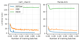
In addition, we compare IKFlow to an Invertible Neural Network (INN) [2] and to a Mixture Density Network (MDN) [4] on two benchmarks—railY_chain3 and Panda Arm. The railY_chain3 robot (first used by Ardizzone et al.), is a planar robot with 4 joints—the first is a prismatic actuator along the y axis with limits [-1, 1]. The final three are revolute joints with limits [, ] and associated arm segments of length 1. For a fair comparison, the IKFlow and INN models have the same number of coupling layers and size of coefficient networks. Further details about the testing procedure are presented in the appendix.
These experiments were carried out on different kinematic chains across different robots, to evaluate the generality of the approach across different kinematic structures.
VI Results
Our results demonstrate that IKFlow provides a representative set of solutions, quickly, with acceptable error. The results of all the experiments can be found in Table II.
VI-A Comparative Evaluation
Benchmarking results are shown in Figure 5. On both test beds, the IKFlow model performs considerably better than the other two models. These results are consistent with previous findings [15], in which it is shown that Conditional INNs (cINNs) outperform INNs on the railY_chain3 testbed. The Panda Arm test bed demonstrates that IKFlow handles higher dimensional problems better than the INN and MDN. The higher the dimension of the problem, the more likely there is to be a lower dimension solution space that would introduce instabilities in training.
VI-B Accuracy
The accuracy of the system output ranges from 7.72mm to 0.36mm and from 2.81 degrees to 0.15 degrees. For a point of reference, the mechanical repeatability of many industrial arms is 0.1mm. This level of accuracy is sufficient for many tasks; additionally these solutions can also be quickly refined with numerical optimization approaches to reach arbitrary levels of precision. For ATLAS - Arm, refinement takes on average 0.20 ms, as presented in Figure 6.
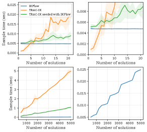
VI-C Runtime
The runtime of the approach is fast enough to enable its use as a sub-routine in other algorithms. Nonlinear optimization approaches find a single solution in about 0.3 millisecond [3], whereas IKFlow can return 500 solutions in 5ms. Figure 6 also demonstrates that the approach scales linearly with the number of requested solution samples. The gradient of the increase is low with samples found in milliseconds. This means that even complex solution sets can be approximated quickly. For a point of comparison, if TRAC-IK, a common nonlinear optimization based IK solver [3], is fed random seeds in hopes that the local minima it finds are different, it takes more than a second to return samples.
Notably however, TRAC-IK takes approximately 5x less time to run when seeded with an approximate solution returned by IKFlow. Empirically, it is faster to first run IKFlow to generate seeds before running TRAC-IK when requesting 7 or more solutions.
VI-D Solution Space Coverage
Figure 3 provides a qualitative comparison of ground truth samples with samples from IKFlow. The solution spaces look quite similar, and provide reference points for the MMD score for other chains. All of the kinematic chains included have a MMD score under . This implies that the IKFlow solution spaces are very similar to the ground truth samples, with only a few erroneous solutions, or small gaps in coverage.
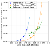
VI-E Limitations
While the proposed method is shown to accurately model kinematic chains with L2 Position error as low as 0.36 mm, it has been found that the training time required for models to reach a given position error grows with the complexity of the kinematic chain that is being modeled. While there exist geometrically derived formulations of kinematic complexity, we choose a simple formulation—the sum of the differences between the upper and lower limits for every joint in the robot:
| (7) |
where and are the upper and lower limits, respectively, for joint . Here this is referred to as the sum of joint limit ranges. An experiment was performed by artificially expanding the joint limits for three robots and measuring the resulting number of training batches required for the respective IKFlow models to reach 1cm of error. The results indicate that the number of training batches required for IKFlow to reach a given L2 error grows exponentially with an increase in equation 7 of the kinematic system it is modeling. The results of this experiment are shown in Figure 8.
VII Conclusion
IKFlow is a novel IK solver capable of providing quick, accurate, and diverse solutions for kinematically redundant robots operating in , based on modeling IK solutions as a distribution over joint poses and using deep generative modeling to model these distributions. Our experiments demonstrated that IKFlow can generate hundreds to thousands of solutions covering the solution space in milliseconds. The average pose error of the results showed that our approach is capable of finding solutions with millimeters of translation error, and less than 1.5 degrees of rotational error. These results demonstrate that IKFlow can serve as the basis for expanded functionality of 7+ DOF kinematic chains.
APPENDIX
VII-A Model and Training Parameters
The coefficient networks are 3x1024-wide fully connected networks with Leaky-Relu activation. A softflow noise scale of was used across all of the models. The learning rate was set to and decayed exponentially by a factor of after every batches. Models were trained until convergence on 2.5 million points using the Ranger optimizer with batch size 128 using a NVIDIA GeForce RTX 2080 Ti graphics card.
VII-B Benchmarking Implementation
For the railY_chain3 test, the IKFlow and INN models both have 6 coupling layers with 3x1024-wide fully connected networks and a latent space dimension of 5. For Panda Arm, both models have 12 coupling layers with 3x1024-wide fully connected coefficient networks and a latent space dimension of 10. The Mixture Density Network (MDN) has 70 and 125 mixture components for the railY_chain3 and Panda arm respectively. MDN models were implemented using the tonyduan/mdn repository [9].
ACKNOWLEDGMENTS
This research was supported in part by DARPA under agreement number D15AP00104, and the ONR under the PERISCOPE MURI Contract N00014-17-1-2699. The content is solely the responsibility of the authors and does not necessarily represent the official views of DARPA. Barrett Ames was partially supported by a NDSEG Fellowship. The authors would like to thank Ben Burchfiel, and Colin Devine for their support of this work.
References
- Almusawi et al. [2016] Ahmed R.J. Almusawi, L. Canan Dülger, and Sadettin Kapucu. A New Artificial Neural Network Approach in Solving Inverse Kinematics of Robotic Arm (Denso VP6242). Computational Intelligence and Neuroscience, 2016, 2016. ISSN 16875273. doi: 10.1155/2016/5720163. URL /pmc/articles/PMC5005769//pmc/articles/PMC5005769/?report=abstracthttps://www.ncbi.nlm.nih.gov/pmc/articles/PMC5005769/.
- Ardizzone et al. [2019] Lynton Ardizzone, Jakob Kruse, Sebastian Wirkert, Daniel Rahner, Eric W. Pellegrini, Ralf S. Klessen, Lena Maier-Hein, Carsten Rother, and Ullrich Köthe. Analyzing inverse problems with invertible neural networks. In International Conference on Representation Learning. arXiv, 8 2019. URL https://arxiv.org/abs/1808.04730v3.
- Beeson and Ames [2015] Patrick Beeson and Barrett Ames. TRAC-IK: An open-source library for improved solving of generic inverse kinematics. In IEEE-RAS International Conference on Humanoid Robots, volume 2015-December, pages 928–935. IEEE Computer Society, 12 2015. ISBN 9781479968855.
- Bishop [1994] Christopher M Bishop. Mixture Density Networks. 1994. URL http://www.ncrg.aston.ac.uk/.
- Csiszar et al. [2017] Akos Csiszar, Jan Eilers, and Alexander Verl. On solving the inverse kinematics problem using neural networks. In 2017 24th International Conference on Mechatronics and Machine Vision in Practice, M2VIP 2017, volume 2017-December, pages 1–6. Institute of Electrical and Electronics Engineers Inc., 12 2017. ISBN 9781509065462. doi: 10.1109/M2VIP.2017.8211457.
- Dai et al. [2019] Hongkai Dai, Gregory Izatt, and Russ Tedrake. Global inverse kinematics via mixed-integer convex optimization. International Journal of Robotics Research, 38(12-13):1420–1441, 10 2019. ISSN 17413176. doi: 10.1177/0278364919846512.
- Demby’S et al. [2019] Jacket Demby’S, Yixiang Gao, and G. N. Desouza. A Study on Solving the Inverse Kinematics of Serial Robots using Artificial Neural Network and Fuzzy Neural Network. In IEEE International Conference on Fuzzy Systems, volume 2019-June. Institute of Electrical and Electronics Engineers Inc., 6 2019. ISBN 9781538617281. doi: 10.1109/FUZZ-IEEE.2019.8858872.
- Diankov [2010] Rosen Diankov. Automated Construction of Robotic Manipulation Programs. PhD thesis, Carnegie Mellon University, Pittsburgh, 2010.
- [9] Tony Duan. GitHub - tonyduan/mdn: Mixture density network implemented in PyTorch. URL https://github.com/tonyduan/mdn.
- Gretton et al. [2012] Arthur Gretton, Karsten M Borgwardt, Malte J Rasch, Alexander Smola, and Bernhard Schölkopf. A Kernel Two-Sample Test. Journal of Machine Learning Research, 13:723–773, 2012. URL www.gatsby.ucl.ac.uk/.
- Kim et al. [2020] Hyeongju Kim, Hyeonseung Lee, Woo Hyun Kang, Joun Yeop Lee, and Nam Soo Kim. SoftFlow: Probabilistic Framework for Normalizing Flow on Manifolds. Technical report, 2020. URL https://github.com/ANLGBOY/SoftFlow.
- Kim and Perez [2021] Seungsu Kim and Julien Perez. Learning Reachable Manifold and Inverse Mapping for a Redundant Robot manipulator. In International Conference on Robotics and Automation, pages 4731–4737. Institute of Electrical and Electronics Engineers (IEEE), 10 2021. ISBN 9781728190778. doi: 10.1109/ICRA48506.2021.9561589.
- Kingma and Dhariwal [2018] Diederik P Kingma and Prafulla Dhariwal. Glow: Generative Flow with Invertible 1×1 Convolutions. In 32nd Conference on Neural Information Processing Systems, 2018. URL https://github.com/openai/glow.
- Kobyzev et al. [2021] Ivan Kobyzev, Simon J.D. Prince, and Marcus A. Brubaker. Normalizing Flows: An Introduction and Review of Current Methods. IEEE Transactions on Pattern Analysis and Machine Intelligence, 43(11):3964–3979, 11 2021. ISSN 19393539. doi: 10.1109/TPAMI.2020.2992934.
- Kruse et al. [2019] Jakob Kruse, Lynton Ardizzone, Carsten Rother, and Ullrich Köthe. Benchmarking Invertible Architectures on Inverse Problems. In Workshop on Invertible Neural Networks and Normalizing Flows, 2019.
- Papamakarios et al. [2019] George Papamakarios, Eric Nalisnick, Danilo Jimenez Rezende, Shakir Mohamed, and Balaji Lakshminarayanan. Normalizing Flows for Probabilistic Modeling and Inference. Journal of Machine Learning Research, 12 2019. URL http://arxiv.org/abs/1912.02762.
- Paszke et al. [2019] Adam Paszke, Sam Gross, Francisco Massa, Adam Lerer, James Bradbury, Gregory Chanan, Trevor Killeen, Zeming Lin, Natalia Gimelshein, Luca Antiga, Alban Desmaison, Andreas Köpf Xamla, Edward Yang, Zach Devito, Martin Raison Nabla, Alykhan Tejani, Sasank Chilamkurthy, Qure Ai, Benoit Steiner, Fang Lu, Bai Junjie, and Soumith Chintala. PyTorch: An Imperative Style, High-Performance Deep Learning Library. Technical report, 2019.
- Rakita et al. [2019] Daniel Rakita, Bilge Mutlu, and Michael Gleicher. STAMPEDE: A Discrete-Optimization Method for Solving Pathwise-Inverse Kinematics. In International Conference on Robotics and Automation, 2019.
- Ren and Ben-Tzvi [2020] Hailin Ren and Pinhas Ben-Tzvi. Learning inverse kinematics and dynamics of a robotic manipulator using generative adversarial networks. Robotics and Autonomous Systems, 124:103386, 2 2020. ISSN 09218890. doi: 10.1016/j.robot.2019.103386.
- Rezende and Mohamed [2015] Danilo Jimenez Rezende and Shakir Mohamed. Variational Inference with Normalizing Flows. In Proceedings of the 32nd International Conference on Machine Learning, 2015.
- Rezende et al. [2020] Danilo Jimenez Rezende, George Papamakarios, Sébastien Racanière, Michael S. Albergo, Gurtej Kanwar, Phiala E. Shanahan, and Kyle Cranmer. Normalizing Flows on Tori and Spheres. In International Conference on Machine Learning, 2 2020. URL http://arxiv.org/abs/2002.02428.
- Zhang and Hannaford [2017] Dianmu Zhang and Blake Hannaford. IKBT: solving closed-form Inverse Kinematics with Behavior Tree. Journal of Artificial Intelligence Research, 65, 11 2017.