IAAT: A Input-Aware Adaptive Tuning framework for Small GEMM

Jianyu Yao12, Boqian Shi3, Chunyang Xiang124, Haipeng Jia14, Chendi Li12, Hang Cao12, Yunquan Zhang1 1SKL of Computer Architecture, Institute of Computing Technology, Chinese Academy of Sciences, Beijing, China 2University of Chinese Academy of Sciences, Beijing, China 3Indiana University Bloomington, Indiana, USA 4Corresponding Author {yaojianyu19f, xiangchunyang, jiahaipeng, lichendi19s, caohang, zyq}@ict.ac.cn, [email protected]

Abstract

GEMM with the small size of input matrices is becoming widely used in many fields like HPC and machine learning. Although many famous BLAS libraries already supported small GEMM, they cannot achieve near-optimal performance. This is because the costs of pack operations are high and frequent boundary processing cannot be neglected. This paper proposes an input-aware adaptive tuning framework(IAAT) for small GEMM to overcome the performance bottlenecks in state-of-the-art implementations. IAAT consists of two stages, the install-time stage and the run-time stage. In the run-time stage, IAAT tiles matrices into blocks to alleviate boundary processing. This stage utilizes an input-aware adaptive tile algorithm and plays the role of runtime tuning. In the install-time stage, IAAT auto-generates hundreds of kernels of different sizes to remove pack operations. Finally, IAAT finishes the computation of small GEMM by invoking different kernels, which corresponds to the size of blocks. The experimental results show that IAAT gains better performance than other BLAS libraries on ARMv8 platform.

Index Terms:

Small GEMM, Matrix Multiplication, Code Generation

I Introduction

General matrix multiplication(GEMM), as one of the most important numerical algorithm in dense linear algebra, has been exhaustively studied over the years[1, 2, 3]. Many famous BLAS(Basic Linear Algebra Subprograms) libraries, like Intel MKL[4], OpenBLAS[2], BLIS[3], and ARMPL[5], already implemented high-performance GEMM. GEMM is used to compute $C=\alpha A\times B+\beta C$ . Here $C$ , $A$ , $B$ are $M\times N$ , $M\times K$ , and $K\times N$ matrices, respectively.

In recent years, small GEMM becomes more and more important in many fields, such as machine learning[6], sparse matrix[7], and fluid dynamics[8]. Many CNNs algorithms use the small matrix on their fully connected layers[9, 10]. Caffe [11] is a famous deep learning framework. Comparing to BLIS that has not optimized small GEMM, the performance of Caffe utilized optimized BLIS can obtain a performance improvement of 17%[12]. By using the optimized implementation of small GEMM, Geoffrey Hinton reduced the number of parameters by a factor of 15 to 310K compared with their baseline CNN with 4.2M parameters [6]. In this paper, we define small GEMM as, $\sqrt[3]{MNK}\leq 80$ , when transposition of input matrices is not TN(TN will be explained in TABLE I), or $\sqrt[3]{MNK}\leq 32$ when transposition of input matrices is TN. This definition will be explained in Section VI.

Traditional implementation and optimization methods of GEMM mainly have three steps: block step, pack step and compute step. Block step tiles matrices into a series of small blocks based on features of the hardware, e.g., TLB, size of the L2 cache. Pack step packs these small blocks based on kernel size to ensure continuity of memory access during kernel calculation. Compute step uses one high-performance kernel with boundary processing to compute matrix multiplication. Because input matrices are relatively large, pack step can massively reduce cache miss and TLB miss, and costs of boundary processing can be neglected.

However, traditional implementation and optimization methods of GEMM, as described above, cannot achieve optimal performance for small GEMM. Here are two reasons for this. First, the overhead of pack step in small GEMM is too high, as shown in Section VI. The advantages of pack step are no longer significant, but it results in high extra memory access overhead. Second, the costs of boundary processing are not neglected for small GEMM. Therefore, designing and implementing a method without pack steps and boundary processing is very necessary for achieving high performance of small GEMM.

This paper proposes an input-aware adaptive tuning framework(IAAT) for small GEMM to achieve near-optimal performance. IAAT has two stages, the install-time stage and the run-time stage. The install-time stage is responsible for auto-generating high-performance assembly kernels of different sizes. This stage automatically tunes kernels based on features of hardware to achieve optimal performance. The run-time stage’s core is the input-aware adaptive tile algorithm, which tiles input matrices into some small blocks. This stage plays the role of runtime tuning by tiling matrix during program execution. Our performance evaluation shows that IAAT can achieve near-optimal performance when the size of input matrices is small as shown in Section VI.

Our contributions are summarized as follows:

•

We propose a template-based high-performance code auto-generation method to generate high-performance kernels for GEMM of different sizes in assembly language.
•

We design an input-aware adaptive algorithm to divide input matrices into blocks in runtime to obtain a near-optimal solution.
•

We implement a high-performance input-aware adaptive tuning framework(IAAT) for small GEMM based on ARMv8.

The remainder of this paper is organized as follows. Section II presents related works. Section III provides an overview of the framework. Section IV and Section V introduces the details of two stages of IATT. Section VI presents the experimental results. Finally, Section VII concludes the paper.

II Related Works

Matrix multiplication has been optimized over years. Researchers utilize different methods and technologies to improve various matrix multiplication, such as tall and skinny matrix multiplication[13, 14, 15], batches of matrix multiplication[16, 17], parallel matrix multiplication[18] and so on. For example, tall and skinny matrix multiplication kernels are optimized by a flexible, configurable mapping scheme and outperform on an NVIDIA Volta GPGPU[19]. Lionel Eyraud-Dubois[20] uses more general allocations to perform matrix multiplication on a heterogeneous node based on task-based runtime systems.

Small GEMM are becoming more and more important in recent years. The optimization of small GEMM is introduced by many libraries, like LIBXSMM[21], BLIS[22, 23]. LIBXSMM uses a code generator that has a built-in architectural model to auto-generate code. And the code runs well without requiring an auto-tuning phase by utilizing just-in-time compilation. BLIS uses the method of optimizing skinny matrix to optimize the small matrix and works well[23].

However, current methods and implementations of small GEMM cannot achieve near-optimal performance on ARMv8 platform. LIBXSMM and BLIS only focused on x86 CPU. Besides, BLIS tile algorithm cannot improve the performance of small GEMM to optimal performance of small GEMM[23]. And BLIS only implemented the small GEMM for single-precision and double-precision but not single-precision complex and double-precision complex. Distinguish from LIBXSMM and BLIS, we optimize all types of small GEMM for ARMv8 platform.

Refer to caption — Figure 1: The overall IAAT

III Framework

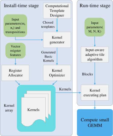
This section introduces the input-aware adaptive tuning framework(IAAT), as shown in Fig.1, with two stages, the install-time stage and the run-time stage to achieve near-optimal performance for small GEMM.

III-A The Install-Time Stage

The install-time stage auto-generates hundreds of kernels of different sizes. Pack step of the traditional method of GEMM makes data access continuous. So the traditional method of GEMM only needs one kernel to accomplish computation for different transpositions. After removing pack step, we have to use hundreds of kernels for different matrix sizes, types and transpositions. These kernels need lots of work to write by hand. Therefore, IAAT uses auto-generation to generate high-performance kernels in the install-time stage. This stage automatically tunes kernels based on features of the hardware to achieve optimal performance. The install-time stage utilizes four components to generate kernels:

•

Computational Template Designer abstracts typical computing patterns of matrix multiplication as templates.
•

Kernel Generator designs a kernel generation algorithm, which utilizes templates from compute template designer to generate basic kernels of different sizes.
•

Register Allocator allocates SIMD registers for kernels based on the size of kernel and SIMD register features.
•

Kernel Optimizer optimizes kernels from kernel generator to approach full potential power of the hardware.

TABLE I: ALL GENERATED KERNELS

SGEMM

\times

{1,2,3,4}

\times

{1,2,…,6}

\times

{1,2,…,8}

\times

{1,2,…,13}

\times

{1,2,…,13}

\times

{1,2,…,13}

\times

{1,2,…,13}

\times

{1,2,3,4}

\times

{1,2,…,8}

\times

{1,2,…,8}

\times

{1,2,…,20}

\times

{1,2,…,24}

\times

{1,2,…,28}

\times

{1,2,…,32}

\times

{1,2,3,4}

\times

{1,2,3,4,5}

\times

{1,2,…,7}

\times

{1,2,…,10}

{1,2,3,4}

\times

{1,2,…,6}

\times

{1,2,…,8}

\times

{1,2,…,13}

\times

{1,2,…,13}

\times

{1,2,…,13}

\times

{1,2,…,13}

\times

DGEMM

\times

{1,2,3,4}

\times

{1,2,…,8}

\times

{1,2,…,8}

\times

{1,2,…,15}

\times

{1,2,…,15}

\times

{1,2,3,4}

\times

{1,2,…,8}

\times

{1,2,…,8}

\times

{1,2,…,20}

\times

{1,2,…,20}

\times

{1,2,3,4}

\times

{1,2,3,4,5}

\times

{1,2,…,7}

\times

{1,2,…,10}

{1,2,3,4}

\times

{1,2,…,8}

\times

{1,2,…,8}

\times

{1,2,…,15}

\times

{1,2,…,15}

\times

CGEMM

\times

{1,2,3,4}

\times

{1,2,…,9}

\times

{1,2,…,9}

\times

{1,2,…,12}

\times

{1,2,…,20}

\times

{1,2,3,4}

\times

{1,2,…,8}

\times

{1,2,…,8}

\times

{1,2,…,12}

\times

{1,2,…,20}

\times

{1,2,…,9}

\times

{1,2,…,9}

\times

{1,2,…,12}

\times

{1,2,…,20}

{1,2,3,4}

\times

{1,2,…,9}

\times

{1,2,…,9}

\times

{1,2,…,12}

\times

{1,2,…,20}

\times

ZGEMM

\times

{1,2,3,4}

\times

{1,2,3,4}

\times

{1,2,…,7}

\times

{1,2,…,10}

\times

{1,2,3,4}

\times

{1,2,3,4}

\times

{1,2,…,7}

\times

{1,2,…,10}

\times

{1,2,3,4}

\times

{1,2,3,4}

\times

{1,2,…,7}

\times

{1,2,…,10}

{1,2,3,4}

\times

{1,2,3,4}

\times

{1,2,…,7}

\times

{1,2,…,10}

\times

We define the kernel for different matrix types and different transpositions. The SGEMM/DGEMM/CGEMM/ZGEMM represent single-precision matrix multiplication, double-precision matrix multiplication, single-precision complex matrix multiplication, double-precision complex matrix multiplication. Each type has four transpositions, NN, NT, TN, and TT. For example, NT means matrix A is not transposed and matrix B is transposed. We will also use abbreviations like SGEMM_TN, which means input matrix type is single and matrix A is transposed and matrix B isn’t transposed. We acquiescence the matrix in column-major order.

TABLE I shows all kernels we defined in this paper, which are completely auto-generated. All these kernels construct basic computation of small GEMM and form a kernel array, which is directly invoked by the run-time stage.

III-B The Run-Time Stage

The run-time stage tiles input matrices A, B, and C into blocks and generates a near-optimal small GEMM kernel executing plan. The costs of boundary processing can be neglected for GEMM. However, for small GEMM, the costs of boundary processing are high and cannot be neglected. To reduce or eliminate boundary processing, an algorithm is required, which can tile input matrices into optimal blocks with less boundary processing. The core of the run-time stage is the input-aware adaptive tile algorithm. This algorithm tiles input matrices into optimal blocks according to the size of kernels from the install-time stage. These blocks are tuned according to input matrix sizes, types and transpositions. Therefore, the run-time stage plays the role of runtime tuning. Then this stage connects the kernel to form a sequence of kernels, which is called the kernel executing plan. Finally, IAAT computes the small GEMM based on this kernel executing plan.

IV The Install-Time Stage

This section focuses on the install-time stage, which auto-generates hundreds of kernels of different sizes. Below we introduce four components of the install-time stage as shown in Fig.1.

IV-A Computational Template Designer

To construct main calculation of GEMM kernel, we introduce computational template designer. The computational template designer extracts typical computing patterns of matrix multiplication as templates, which are shown in TABLE II.

•

sfmlas and dfmlas represent a vector-scalar multiply-add operation.
•

sfmlav and dfmlav represent a vector-vector multiply-add operation.
•

sfmlss and dfmlss represent a vector-scalar multiplication and subtraction.
•

sfnegv and dfnegv are used to invert values in register.
•

sfcmlas and dfcmlas represent a vector-scalar complex multiply-add operation.
•

sfcmlav and dfcmlav represent a vector-vector complex multiply-add operation.

TABLE II: Kernel Computational Templates

sfmlas(out, in1, in2, index):

fmla out.4s, in1.4s, in2.s[index]

dfmlas(out, in1, in2, index):

fmla out.2d, in1.2d, in2.d[index]

sfmlav(out, in1, in2):

fmla out.4s, in1.4s, in2.4s

dfmlav(out, in1, in2):

fmls out.2d, in1.2d, in2.2d

sfmlss(out, in1, in2, index):

fmls out.4s, in1.4s, in2.s[index]

dfmlss(out, in1, in2, index):

fmla out.2d, in1.2d, in2.d[index]

sfnegv(out, in1):

fneg out.4s, in1.4s

dfnegv(out, in1):

fneg out.2d, in1.2d

sfcmlas(out, in1, in2, index, rot[2]):

fcmla out.4s, in1.4s, in2.s[index], rot[0]

fcmla out.4s, in1.4s, in2.s[index], rot[1]

dfcmlas(out, in1, in2, rot[2]):

fcmla out.2d, in1.2d, in2.2d, rot[0]

fcmla out.2d, in1.2d, in2.2d, rot[1]

sfcmlav(out, in1, in2, rot[2]):

fcmla out.4s, in1.4s, in2.4s, rot[0]

fcmla out.4s, in1.4s, in2.4s, rot[1]

dfcmlav(out, in1, in2, rot[2]):

fcmla out.2d, in1.2d, in2.2d, rot[0]

fcmla out.2d, in1.2d, in2.2d, rot[1]

IV-B Kernel Generator

Kernel generator is responsible for generating kernels. These kernels are used to compute $C_{c}=A_{c}\times B_{c}+Cc$ . Here $A_{c}$ , $B_{c}$ , and $C_{c}$ are blocks of input matrices A, B, and C. And they are $m_{c}\times k_{c}$ , $k_{c}\times n_{c}$ , and $m_{c}\times n_{c}$ matrices, respectively. The algorithm of kernel generator takes size of $C_{c}$ as input and outputs high-performance kernel in assembly language.

Kernel generator generates two kinds of subkernels for ping-pang operation. The ping-pang operation is an optimization method that split the multiplication into two stages, M1 and M2 stages. There are two types of ping-pang operations. In the first type, each stage of ping-pang operation multiplies a column of block $A_{c}$ and a row of block $B_{c}$ and loads the next column of block $A_{c}$ and next row of block $B_{c}$ . In the second type, each stage multiplies a column of block $A_{c}$ and a row of block $B_{c}$ , M1 stage loads the next column of block $A_{c}$ and two rows of block $B_{c}$ , and M2 stage loads the next column of block $A_{c}$ . And the performance difference between these two types is not too much.

The kernel generator algorithms for various input matrix types and transpositions are similar. We only discuss SGEMM_NN kernel generator shown in Algorithm 1.

SGEMM_NN kernel generator generates two subkernels in lines 6-12 and 14-19. The first subkernel loads a column of $A_{c}$ and two rows of $B_{c}$ in lines 6-7 and the second subkernel loads a column of $A_{c}$ in line 14. Each subkernel multiplies a column of $A_{c}$ and a row of $B_{c}$ by utilizing sfmlas in lines 8-12 and 15-19.

After two kinds of subkernels of SGEMM_NN are generated, the kernel generator invokes these two subkernels in a loop on the $k_{c}$ dimension and completes the generation of SGEMM_NN kernel.

Algorithm 1 kernel generator of SGEMM_NN

m_{c}

n_{c}

: the size of the input kernel

kernel

Cregs\leftarrow\{C_{1},C_{2},...,C_{m_{\left\lceil m_{c}/4\right\rceil}n_{c}}\}

A1regs\leftarrow\{A_{1},A_{2},...,A_{\left\lceil m_{c}/4\right\rceil}\}

A2regs\leftarrow\{A_{\left\lceil m_{c}/4\right\rceil+1},

A_{\left\lceil m_{c}/4\right\rceil+2},

...,

A_{2\left\lceil m_{c}/4\right\rceil}\}

Bregs\leftarrow\{B_{1},B_{2},...,B_{n_{c}}\}

5: //first subkernel

6: load next column of block

A_{c}

A2regs

7: load two rows of block

B_{c}

Bregs

8: for

i

\leftarrow

0

to

n_{c}

9: for

j

\leftarrow

0

to

\left\lceil m_{c}/4\right\rceil

10: sfmlas(

Cregs{[}i\left\lceil m_{c}/4\right\rceil+j{]}

A1regs{[}j{]}

Bregs{[}i{]}

, 0)

11: end for

12: end for

13: //second subkernel

14: load next column of block

A_{c}

A1regs

15: for

i

\leftarrow

0

to

n_{c}

16: for

j

\leftarrow

0

to

\left\lceil m_{c}/4\right\rceil

17: sfmlas(

Cregs{[}i\left\lceil m_{c}/4\right\rceil+j{]}

A2regs{[}j{]}

Bregs{[}i{]}

, 1)

18: end for

19: end for

IV-C Register Allocator

The allocation of registers is very important for the performance of small GEMM. Hence, we need to define the strategies of register allocation for different kernels. The work of our paper is mainly carried out on ARMv8 platform, which contains 32 128-bit SIMD registers.

The basic idea behind the register allocator is to divide all registers into three groups. $A_{c}$ register group contains two columns of $A_{c}$ ; $B_{c}$ register group contains two rows of $B_{c}$ for ping-pang operation; $C_{c}$ register group holds the whole block $C_{c}$ .

Allocation of the $A_{c}$ register group has four main strategies, ANTwoCC, ATEachCTwo, ATEachCOne, and ATTwoRR.

•

ANTwoCC is for loading two columns of $A_{c}$ to registers. It allocates $2\left\lceil m_{c}/elenum\right\rceil$ registers, the $elenum$ means the number of elements that a register can store.
•

ATEachCTwo is for loading first two data of each column of transposed $A_{c}$ to two registers. It allocates a total of $2m_{c}$ registers.
•

ATEachCOne is for loading first two data of each column of transposed $A_{c}$ to one register. It requires a total of $m_{c}$ registers for single-precision, double-precision, and single-precision complex. As for double-precision complex, it requires a total of $2m_{c}$ registers.
•

ATTwoRR is for loading two rows of transposed $A_{c}$ to registers. It allocates $2\left\lceil m_{c}/elenum\right\rceil$ registers.

The strategies of allocating $B_{c}$ register group are BTTwoCC, BNEachCTwo, BNEachCOne, and BNTwoRR corresponding to ANTwoCC, ATEachCTwo, ATEachCOne, and ATTwoRR. This is because load methods of $A_{c}$ are the same as load methods of $B_{c}$ .

The strategy of allocating the C register group is allocating $\left\lceil m_{c}\times n_{c}/elenum\right\rceil$ registers.

The register allocator has one special strategy for TN transposition that allocates $2m_{c}$ registers for $A_{c}$ and $2n_{c}$ registers for $B_{c}$ . This transposition makes memory access to $A_{c}$ and $B_{c}$ discontinuous. So we cannot vectorize small GEMM for this transposition. Therefore, the methods of loading data are load data from each column of $A_{c}$ by columns and load data from each column of $B_{c}$ by columns.

IV-D Kernel Optimizer

After kernels are generated, kernels will be optimized as follows.

Instruction Choice

Computational template designer utilizes the FMA instruction instead of $mul$ or $add$ because there usually are fused multiply-add(FMA) units in hardware. Besides, we prioritize the $ldp$ and $ldr$ instructions because these two instructions are relatively high-performance.

Instruction Order

The loading instructions are interspersed among the computing instructions. It makes better use of the instruction pipeline to avoid pipeline stalling.

Ping-Pang Operation

As described in Subsection IV-B, this optimization utilizes computing instruction to hide the delay of loading instructions.

V The Run-Time Stage

This section introduces the run-time stage. This stage first tile input matrices and then construct a kernel executing plan to compute small GEMM. The input-aware adaptive tile algorithm is the core of this stage.

V-A Input-Aware Adaptive Tile Algorithm

The input-aware adaptive tile algorithm first tiles input matrix C into some small blocks. Each block has the same size as one of the generated kernels. Then, this algorithm tiles matrices A and B based on tiled blocks of C. This algorithm is based on the three principles listed below.

Algorithm 2 SGEMM_NN Tile Algorithm

M,N,K

: the sizes of input matrices,

kernels

: array of all sorted SGEMM_NN kernels from TABLE I

blocksC

[],

blocksA

[],

blocksB

[]

1: if

N\leq 13

then

m[]\leftarrow(m_{1},I)

m_{1}

is the largest

m_{c}

of kernel that’s

n_{c}

is equal

N

and

I

is an integer and make sure the

m_{1}I\leq M

n[]\leftarrow[(N,1)]

4: if

m_{1}I<M

then

m

.append(

(M-m_{1}I,1)

)

n

.append(

[(N,1)]

)

7: end if

8: else

9: if

M<8

then

10:

m[]\leftarrow TileSingleDim(M,[1,2,3,4])

11:

n[]\leftarrow[TileSingleDim(N,[1,2,...,13])]

12: if size of

m

== 2 then

13:

n.append([TileSingleDim(N,[1,2,...,13])])

14: end if

15: else if

M==9

then

16:

m[]\leftarrow(4,1),(3,1),(2,1)

17:

n[]\leftarrow[TileSingleDim(N,[1,2,...,13])],

[TileSingleDim

(N,

[1,2,...,13])],

[TileSingleDim(N,

[1,2,...,13])]

18: else if

M<12

then

19:

m[]\leftarrow(8,1),(M-8,1)

20:

n[]\leftarrow[TileSingleDim(N,[1,2,...,8])],

[TileSingleDim

(N,

[1,2,...,13])]

21: else if

M==12

then

22:

m[]\leftarrow(12,1)

23:

n[]\leftarrow[TileSingleDim(N,[1,2,3,4,5,6])]

24: else

25:

m_{1}[]\leftarrow(4,\lfloor M/4\rfloor)

26:

m_{2}[]\leftarrow(M-4\lfloor M/4\rfloor,1)

27:

n_{2}[]\leftarrow[TileSingleDim(N,[1,2,...,13])]

28: if

M-4\lfloor M/4\rfloor==1

then

29:

m_{1}[]\leftarrow(4,\lfloor M/4\rfloor-1)

30:

m_{2}[]\leftarrow(3,1),(2,1)

31:

n_{2}[]\leftarrow

[TileSingleDim(N,

[1,2,...,8])],

[TileSingleDim

(N,

[1,2,...,13])]

32: end if

33:

m8\leftarrow ExtendTo8(m_{1})

34:

m16\leftarrow ExtendTo16(m_{1})

35:

n8[]

and

n16[]

\leftarrow

tile

N

m8[]

and

m16[]

36:

blocksC1\leftarrow Combine(m8,n8)

37:

blocksC2\leftarrow Combine(m16,n16)

38:

blocksC\leftarrow CompareLessMemops(blocksC1,blocksC2)

39:

blocksC

.append(combine(

m_{2}

n_{2}

))

40: return

41: end if

42: end if

43:

blocksC\leftarrow Combine(m,n)

44:

blocksA[]\leftarrow

tile matrix A according to

blocksC[]

45:

blocksB[]\leftarrow

tile matrix B according to

blocksC[]

Bigger Block Size

Smaller blocks cause matrices A and B to be repeatedly loaded more times. The larger the block size, the lower the number of repetitions.

Minimal Memops

Different tiling methods have the same amount of computing instructions but different numbers of loading instructions. Therefore, the optimal tiling method is tiling matrices into blocks with the fewest loading instructions. The tiled blocks for matrix C are supposed to be $m_{0}\times n_{0}$ , $m_{1}\times n_{1}$ , …, $m_{i}\times n_{i}$ . The $m_{i}\times n_{i}$ is size of tiled block. This tiling method have a total of $(m_{0}+n_{0}+m_{1}+n_{1}...+m_{a}+n_{a})K+2mn$ data to access from L2 cache to register. So the value of $(m_{0}+n_{0}+m_{1}+n_{1}...+m_{a}+n_{a})$ should be preserved to a bare minimum.

SIMD Friendly

The dimension of block, that data is continuous, can be divisible by the length of SIMD register.

The pseudo-code of SGEMM_NN tile algorithm are shown in Algorithm 2. The outline of this algorithm is below:

When $N\leq 13$ , we let $n_{c}=N$ and make $m_{c}$ the maximum value that $m_{c}$ can be taken in lines 1-7. When $N>13$ , we first tile $M$ into multiples of 4 and use 1, 2, 3 to supplement the deficiency, and then tile $N$ into maximum value that $n_{c}$ can be taken according to the result of $M$ ’s tile in lines 9-42. Besides, when $M>12$ , $M$ can be tiled by 8 or 16 and we compare which one is better by counting the number of loading instructions and choose that. Then, we combine the two tiled dimensions $m[]$ and $n[]$ into $blocksC$ . Finally, we tile matrices A and B into $blocksA$ and $blocksB$ according to blocks of matrix C.

$TileSingleDim$ algorithm, as shown in line 10, is for tiling a single dimension. It takes two input parameters: the length that you want to tile, and the array of lengths that you used to tile. This algorithm outputs array $(dim,nums)$ means $dim$ is repeated $nums$ times. We tile $dim$ into $nums_{1}I+nums_{2}...+nums_{i}$ and the bigger $nums_{1}$ , the better. And if $nums_{i}$ is too small, this algorithm will average $nums_{i-1}$ and $nums_{i}$ .

For various types and transpositions, the specific tile algorithm is changed slightly. But the basic ideas are consistent as shown above.

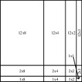
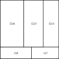
For SGEMM_NN $15\times 15\times K$ matrix, the traditional tiling method is showed in Figure 2(a). This method needs to load $105k+450$ data from L2 cache to register. And, our method tile SGEMM_NN is showed in Figure 2(b). This tiling method needs to load $72K+450$ data. The amount of data loaded by the traditional method is 45% more than that of our method.

V-B Kernel Executing Plan

After input matrices are tiled, IAAT constructs a kernel executing plan by connecting kernels, which correspond to the sizes of tiled blocks. Finally, IAAT executes this plan to compute small GEMM.

VI Performance Evaluation

In this section, we analyze small GEMM’s performance on ARMv8 platform as listed in TABLE III. We compared IAAT with currently state-of-the-art BLAS libraries: OpenBLAS, ARMPL, and BLIS. GEMM in these libraries is well optimized. Our work supports four data types: single-precision, double-precision, single-precision complex, and double-precision complex. Each data type supports four transpositions: NN, NT, TN, TT. Thus, we compared 16 kinds of small GEMMs. We use Equation 1 to evaluate performance of SGEMM and DGEMM and Equation 2 to evaluate performance of CGEMM and ZGEMM.

TABLE III: Experimental Environment Of ARMv8 platform

Hardware	CPU	Kunpeng920
	Arch.	ARMv8.2
	Freq.	2.6GHz
	SIMD	128bits
	L1 cache	4MiB
	L2 cache	32MiB
Software	Compiler	GCC7.5
	OpenBLAS	0.3.13
	ARMPL	21.0
	BLIS	0.81

	$\displaystyle GFLOPS$	$\displaystyle=$	$\displaystyle\frac{2\times M\times N\times K}{t}$		(1)
	$\displaystyle GFLOPS$	$\displaystyle=$	$\displaystyle\frac{2\times 4\times M\times N\times K}{t}$		(2)

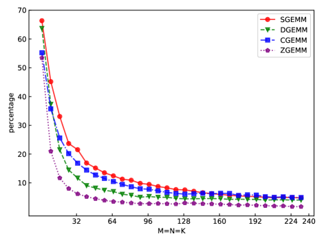
Fig.3 shows proportion of pack step cost in traditional implementation of GEMM. It shows that the proportion of pack step cost can reach 67% when input matrices are very small. As the size of input matrices increases, the proportion decreases exponentially. When input matrices are large enough, the proportion is near 3%.

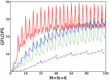
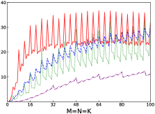
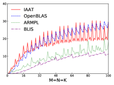
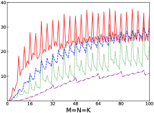
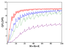
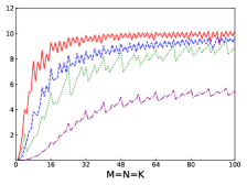
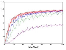
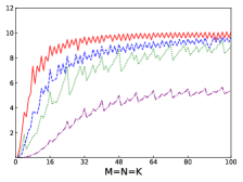
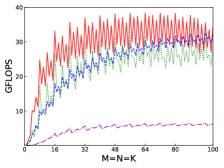
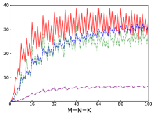
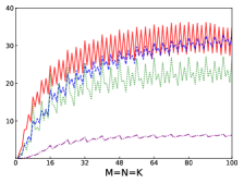
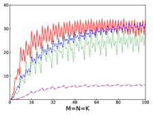
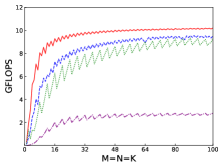
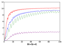
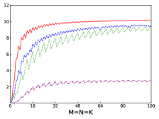
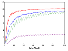
Fig.4 shows performances of NN, NT, TN, TT of SGEMM of IAAT, OpenBLAS, ARMPL, and BLIS. When input matrices are small, IAAT is faster than OpenBLAS, ARMPL, and BLIS for all transpositions. When $M=N=K\leq 80$ and transposition is NN, as shown in Fig.4(a), IAAT is on average 1.81, 2.3, and 20.17 times faster than OpenBLAS, ARMPL, and BLIS, respectively. When $M=N=K\leq 80$ and transposition is NT, as shown in Fig.4(b), IAAT is on average 1.81, 2.29, and 20.19 times faster than OpenBLAS, ARMPL, and BLIS, respectively. When $M=N=K\leq 32$ and transposition is TN, as shown in Fig.4(c), IAAT is on average 1.65 times faster than OpenBLAS. When $M=N=K>32$ and transposition is TN, as shown in Fig.4(c), IAAT is only faster than OpenBLAS when sizes of input matrices are multiples of 4. However, when $M=N=K\leq 100$ and transposition is TN, IAAT is faster than ARMPL and BLIS and is on average 2.15 and 11.57 times, respectively. When $M=N=K\leq 80$ and transposition is TT, as shown in Fig.4(d), IAAT is on average 1.73, 2.55, and 18.76 times faster than OpenBLAS, ARMPL, and BLIS, respectively.

Fig.5 shows performances of NN, NT, TN, TT of DGEMM of IAAT, OpenBLAS, ARMPL, and BLIS. When input matrices are small, IAAT is faster than OpenBLAS, ARMPL, and BLIS for all transpositions. When $M=N=K\leq 80$ and transposition is NN, as shown in Fig.5(a), IAAT is on average 1.48, 1.66, and 15.0 times faster than OpenBLAS, ARMPL, and BLIS, respectively. When $M=N=K\leq 80$ and transposition is NT, as shown in Fig.5(b), IAAT is on average 1.43, 1.66, and 14.56 times faster than OpenBLAS, ARMPL, and BLIS, respectively. When $M=N=K\leq 80$ and transposition is TN, as shown in Fig.5(c), IAAT is on average 1.32, 1.47, and 12.78 times faster than OpenBLAS, ARMPL, and BLIS, respectively. When $M=N=K\leq 80$ and transposition is TT, as shown in Fig.5(d), IAAT is on average 1.43, 1.64, and 14.54 times faster than OpenBLAS, ARMPL, and BLIS, respectively.

Fig.6 shows performances of NN, NT, TN, TT of CGEMM of IAAT, OpenBLAS, ARMPL, and BLIS. When input matrices are small, IAAT is faster than OpenBLAS, ARMPL, and BLIS for all transpositions. When $M=N=K\leq 80$ and transposition is NN, as shown in Fig.6(a), IAAT is on average 1.31, 1.30, and 13.24 times faster than OpenBLAS, ARMPL, and BLIS, respectively. When $M=N=K\leq 80$ and transposition is NT, as shown in Fig.6(b), IAAT is on average 1.37, 1.44, and 13.55 times faster than OpenBLAS, ARMPL, and BLIS, respectively. When $M=N=K\leq 64$ and transposition is TN, as shown in Fig.6(c), IAAT is on average 1.16, 1.33, and 13.68 times faster than OpenBLAS, ARMPL, and BLIS, respectively. When $M=N=K\leq 80$ and transposition is TT, as shown in Fig.6(d), IAAT is on average 1.27, 1.46, and 12.94 times faster than OpenBLAS, ARMPL, and BLIS, respectively.

Fig.7 shows performances of NN, NT, TN, TT of ZGEMM of IAAT, OpenBLAS, ARMPL, and BLIS. When input matrices are small, IAAT is faster than OpenBLAS, ARMPL, and BLIS for all transpositions. When $M=N=K\leq 80$ and transposition is NN, as shown in Fig.7(a), IAAT is on average 1.09, 1.3, and 9.62 times faster than OpenBLAS, ARMPL, and BLIS, respectively. When $M=N=K\leq 80$ and transposition is NT, as shown in Fig.7(b), IAAT is on average 1.09, 1.32, and 9.6 times faster than OpenBLAS, ARMPL, and BLIS, respectively. When $M=N=K\leq 80$ and transposition is TN, as shown in Fig.7(c), IAAT is on average 1.11, 1.32, and 9.69 times faster than OpenBLAS, ARMPL, and BLIS, respectively. When $M=N=K\leq 80$ and transposition is TT, as shown in Fig.7(d), IAAT is on average 1.1, 1.34, and 9.6 times faster than OpenBLAS, ARMPL, and BLIS, respectively. ei In addition to the above performance description, we still observe the following three phenomena.

Firstly, as shown in all Fig. 4, 5, 6, and 7, all performance curves of IAAT are very steep When input matrices are small and tend to be smooth along with increase of size. All performance curves of IAAT relate to the proportion of pack step, as shown in Fig.3. As mentioned in Section I, performance improvement of small GEMM comes from removing pack steps. The greater proportion of pack step cost, the higher performance improvement. For example, when $M=N=K\leq 64$ , the proportion of pack step of SGEMM_NN drops, when $M=N=K>64$ , the curve of proportion is smooth. The corresponding performance curve of SGEMM_NN, as shown in 4(a), rises when $M=N=K\leq 64$ and stops rising when $M=N=K>64$ . The others curve are the same as the curve of SGEMM_NN.

Secondly, performance of TN transposition is not as good as other transpositions as shown in Fig.4, 5, 6 and 7. Because data is not continuous and vectorized computation is not feasible in TN transposition, register allocator has to allocate individual registers for each element of block $C_{c}$ . Therefore, blocks of matrix C occupy too many registers, which causes kernel sizes of SGEMM_TN smaller than other transpositions. We have to tile input matrices into smaller blocks than other transpositions. The number of loading instructions increases significantly. As the size of input matrices increases, the advantage of small GEMM for TN transposition will vanish.

Thirdly, the curves of performance of IAAT, as shown in Fig.4, is wavy. The performance of four transpositions reaches wave crests when the size of input matrices is multiples of 4 and it falls into wave troughs when sizes of input matrices are not multiples of 4. Here are two reasons for this phenomenon. First, Kunpeng920 platform has two fused multiply-add(FMA) units for single but Kunpeng920 cannot fully utilize units. Kunpeng920 can issue two FMA instructions or issue one FMA instruction and one loading instruction at the same time. Therefore, for a kernel of any size, the lower the proportion of loading instructions, the closer the performance is to the peak performance. When the size of the kernel is multiples of 4, the kernel can achieve better performance. When the sizes of input matrices are not multiples of 4, the tile algorithm tiles matrix into blocks, which corresponds to the low performance of kernel. Second, it is because only when the size of input matrices is multiples of 4, small GEMM can make full use of the registers. As one register can store four floats, other sizes of input matrices lead to insufficient register utilization. Therefore, the implementation of small GEMM for input matrices whose size is multiples of 4 has better performance. Similar waves occur in CGEMM as shown in Fig.6, which has the same reasons as SGEMM. Besides, compared with SGEMM and CGEMM, curves of DGEMM and ZGEMM, as shown in Fig.5 and Fig.7, are more smooth and the performance curve of DGEMM and ZGEMM reaches wave crest when the size of input matrices is multiples of 2. Because Kunpeng920 platform has one fused multiply-add(FMA) unit for double, which can be fully utilized. Besides, it is also because the size of data type of DGEMM and ZGEMM is bigger than that of SGEMM and CGEMM. DGEMM and ZGEMM can make better use of registers than SGEMM and CGEMM.

Consider the above performance results, we conclude that our implementation is faster than the others library when the size of input matrices is small enough. As shown by above performance analysis, we define small GEMM, as $\sqrt[3]{MNK}\leq 80$ , when transposition of input matrices is not TN, or $\sqrt[3]{MNK}\leq 32$ when transposition of input matrices is TN as mentioned in Section I.

VII Conclusions

In this paper, we propose the input-aware adaptive tuning framework(IAAT) for small GEMM with two stages: the install-time stage and the run-time stage. The install-time stage auto-generates assembly kernels for ARMv8 platform and the run-time stage tiles input matrices into blocks. Finally, IAAT constructs a kernel executing plan by connecting kernels, which corresponds to the sizes of tiled blocks. As shown in the experiment, IAAT utilizes code generation and adaptive tuning to achieves near-optimal performance for small GEMM. IAAT fits the situation where computes matrix multiplication with the same size repeatedly. Our future work will focus on extending IAAT to other platforms.

Acknowledgements

We would like to express our gratitude to all reviewer’s constructive comments for helping us polish this article. This work is supported by the National Key Research and Development Program of China under Grant Nos.2017YFB0202105, the National Natural Science Foundation of China under Grant No.61972376 and the Natural Science Foundation of Beijing under Grant No.L182053.

References

[1] K. Goto and R. A. v. d. Geijn, “Anatomy of high-performance matrix multiplication,” ACM Transactions on Mathematical Software (TOMS), vol. 34, no. 3, pp. 1–25, 2008.
[2] Q. Wang, X. Zhang, Y. Zhang, and Q. Yi, “Augem: automatically generate high performance dense linear algebra kernels on x86 cpus,” in SC’13: Proceedings of the International Conference on High Performance Computing, Networking, Storage and Analysis. IEEE, 2013, pp. 1–12.
[3] F. G. Van Zee and R. A. Van De Geijn, “Blis: A framework for rapidly instantiating blas functionality,” ACM Transactions on Mathematical Software (TOMS), vol. 41, no. 3, pp. 1–33, 2015.
[4] Intel. Developer reference for intel® oneapi math kernel library - c. [Online]. Available: https://software.intel.com/content/www/us/en/develop/documentation/onemkl-developer-reference-c/top/blas-and-sparse-blas-routines.html
[5] A. Developer. Get started with arm performance libraries. [Online]. Available: https://developer.arm.com/tools-and-software/server-and-hpc/downloads/arm-performance-libraries/get-started-with-armpl-free-version
[6] G. E. Hinton, S. Sabour, and N. Frosst, “Matrix capsules with em routing,” in International conference on learning representations, 2018.
[7] U. Borštnik, J. VandeVondele, V. Weber, and J. Hutter, “Sparse matrix multiplication: The distributed block-compressed sparse row library,” Parallel Computing, vol. 40, no. 5-6, pp. 47–58, 2014.
[8] B. D. Wozniak, F. D. Witherden, F. P. Russell, P. E. Vincent, and P. H. Kelly, “Gimmik—generating bespoke matrix multiplication kernels for accelerators: Application to high-order computational fluid dynamics,” Computer Physics Communications, vol. 202, pp. 12–22, 2016.
[9] W. Ding, Z. Huang, Z. Huang, L. Tian, H. Wang, and S. Feng, “Designing efficient accelerator of depthwise separable convolutional neural network on fpga,” Journal of Systems Architecture, vol. 97, pp. 278–286, 2019.
[10] R. Wang, Z. Yang, H. Xu, and L. Lu, “A high-performance batched matrix multiplication framework for gpus under unbalanced input distribution,” The Journal of Supercomputing, pp. 1–18, 2021.
[11] BAIR. Caffe — deep learning framework. [Online]. Available: https://caffe.berkeleyvision.org/
[12] S. Thangaraj, K. Varaganti, K. Puttur, and P. Rao, “Accelerating machine learning using blis,” 2017.
[13] J. Chen, N. Xiong, X. Liang, D. Tao, S. Li, K. Ouyang, K. Zhao, N. DeBardeleben, Q. Guan, and Z. Chen, “Tsm2: optimizing tall-and-skinny matrix-matrix multiplication on gpus,” in Proceedings of the ACM International Conference on Supercomputing, 2019, pp. 106–116.
[14] C. Rivera, J. Chen, N. Xiong, J. Zhang, S. L. Song, and D. Tao, “Tsm2x: High-performance tall-and-skinny matrix–matrix multiplication on gpus,” Journal of Parallel and Distributed Computing, vol. 151, pp. 70–85, 2021.
[15] C. Li, H. Jia, H. Cao, J. Yao, B. Shi, C. Xiang, J. Sun, P. Lu, and Y. Zhang, “Autotsmm: An auto-tuning framework for building high-performance tall-and-skinny matrix-matrix multiplication on cpus,” in 2021 IEEE Intl Conf on Parallel & Distributed Processing with Applications, Big Data & Cloud Computing, Sustainable Computing & Communications, Social Computing & Networking (ISPA/BDCloud/SocialCom/SustainCom). IEEE, 2021, pp. 159–166.
[16] A. Abdelfattah, S. Tomov, and J. Dongarra, “Matrix multiplication on batches of small matrices in half and half-complex precisions,” Journal of Parallel and Distributed Computing, vol. 145, pp. 188–201, 2020.
[17] A. Abdelfattah and Tomov, “Fast batched matrix multiplication for small sizes using half-precision arithmetic on gpus,” in 2019 IEEE International Parallel and Distributed Processing Symposium (IPDPS). IEEE, 2019, pp. 111–122.
[18] H. Kang, H. C. Kwon, and D. Kim, “Hpmax: heterogeneous parallel matrix multiplication using cpus and gpus,” Computing, vol. 102, no. 12, pp. 2607–2631, 2020.
[19] D. Ernst, G. Hager, J. Thies, and G. Wellein, “Performance engineering for real and complex tall & skinny matrix multiplication kernels on gpus,” The International Journal of High Performance Computing Applications, vol. 35, no. 1, pp. 5–19, 2021.
[20] L. Eyraud-Dubois and T. Lambert, “Using static allocation algorithms for matrix matrix multiplication on multicores and gpus,” in Proceedings of the 47th International Conference on Parallel Processing, 2018, pp. 1–10.
[21] A. Heinecke, G. Henry, M. Hutchinson, and H. Pabst, “Libxsmm: accelerating small matrix multiplications by runtime code generation,” in SC’16: Proceedings of the International Conference for High Performance Computing, Networking, Storage and Analysis. IEEE, 2016, pp. 981–991.
[22] the Science of High-Performance Computing (formerly FLAME) group. Blas-like library instantiation software framework. [Online]. Available: https://github.com/flame/blis
[23] F. G. V. Zee, “The blis approach to skinny matrix multiplication,” https://www.cs.utexas.edu/users/flame/BLISRetreat2019/slides/Field.pdf, 2019.