Hypergraph-based Motion Generation with Multi-modal Interaction Relational Reasoning
Abstract
The intricate nature of real-world driving environments, characterized by dynamic and diverse interactions among multiple vehicles and their possible future states, presents considerable challenges in accurately predicting the motion states of vehicles and handling the uncertainty inherent in the predictions. Addressing these challenges requires comprehensive modeling and reasoning to capture the implicit relations among vehicles and the corresponding diverse behaviors. This research introduces an integrated framework for autonomous vehicles (AVs) motion prediction to address these complexities, utilizing a novel Relational Hypergraph Interaction-informed Neural mOtion generator (RHINO). RHINO leverages hypergraph-based relational reasoning by integrating a multi-scale hypergraph neural network to model group-wise interactions among multiple vehicles and their multi-modal driving behaviors, thereby enhancing motion prediction accuracy and reliability. Experimental validation using real-world datasets demonstrates the superior performance of this framework in improving predictive accuracy and fostering socially aware automated driving in dynamic traffic scenarios.
keywords:
Interaction representation, hypergraph, relational reasoning, multi-modal prediction, motion prediction, motion generation[label1]organization=Center for Geospatial Sciences, Applications, and Technology and Department of Landscape of Architecture and Urban Planning, Texas A&M University,addressline=788 Ross St, city=College Station, postcode=77840, state=TX, country=United States \affiliation[label2]organization=Zachry Department of Civil and Environmental Engineering, Texas A&M University,addressline=201 Dwight Look Engineering Building, city=College Station, postcode=77843, state=TX, country=United States \affiliation[label3]organization=Department of Civil and Environmental Engineering, University of Wisconsin-Madison,addressline=1415 Engineering Dr, city=Madison, postcode=53706, state=WI, country=United States
1 Introduction
Understanding traffic interactions and the way they affect future vehicle trajectories is inherently complex [1]. In mixed traffic environments, where human-driven and automated vehicles coexist, this complexity is amplified, requiring precise interaction representation and behavior modeling for reliable motion prediction [2, 3, 4]. These scenarios often present dynamic interaction topologies with underlying relations, with interaction patterns as well topologies continuously evolving depending on the surrounding context as exampled by lane change maneuvers [5, 6]. These relationships play a crucial role in guiding each vehicle’s decision-making processes. Additionally, each vehicle can display multiple possible modalities in driving intentions and behaviors, including both longitudinal (e.g., acceleration and braking) and lateral (e.g., lane-changing and lane-keeping) maneuvers [7, 8]. Furthermore, collective behaviors, arising from interactions within a group of vehicles and encompassing both cooperative and competitive behaviors [9, 10, 12, 11], further complicate the understanding of these interactions[13, 14, 15]. Figure 1 describes the interaction among multi-vehicles and the corresponding multi-modal driving behaviors. Therefore, it is necessary to model the interaction and multi-modality and reason the interaction relation to accurately capture interactions and forecast their future behaviors [16, 17, 18].

Efforts have been made to address the challenges of vehicle interactions and driving behavior multi-modality. Three primary approaches have been developed: social operation methods, attention-driven methods, and graph-based techniques. Social operations use pooling mechanisms to generate socially acceptable trajectories by capturing the influence of surrounding agents [20, 21]. Attention-driven approaches use attention mechanisms to dynamically weigh neighboring agents’ information [22, 23, 24]. Graph-based methods leverage graph structures to model non-Euclidean spatial dependencies, effectively handling varying interaction topologies and predicting dynamic interactions [25, 26, 27, 28]. These complex interactions create uncertainty, complicating the accurate forecasting of a single future trajectory with high confidence due to varying driving behaviors in identical situations [29, 30], driven by individual driver characteristics and psychological factors. Addressing the multi-modality of driving behaviors often involves introducing latent variables, categorized into those with explicit semantics and those without. Models with explicit semantics use latent variables to clearly represent driving intentions, identifying specific maneuvers and behaviors for multi-modal trajectory predictions [30, 31, 32]. Conversely, models without explicit semantics employ generative deep learning techniques, such as Variational Autoencoders (VAEs) [33] and Generative Adversarial Networks (GANs) [21, 34], to produce diverse trajectories by adding noise to encoded features. While these models generate a wide range of possible trajectories, they often struggle with issues related to interpretability and identifying the most effective strategies for sampling from the generated trajectories.
Despite the advances in modeling vehicle interactions and probabilistically forecasting multi-modal future trajectories, the inherent complexity of social dynamics in traffic systems continues to present significant challenges, with limitations arising from the complex nature of agent interactions in two key aspects: First, prevailing methods primarily focus on pair-wise interactions rather group-wise interactions. In multi-vehicle systems, dynamic interactions among vehicles often exhibit cooperative and competitive behaviors [9, 10, 35, 36], which have been rarely explored. Effectively capturing the collective influence of vehicle groups is vital for understanding complex social dynamics, especially in scenarios where vehicles engage in multi-modal behaviors such as lane changes, acceleration, and deceleration. In such contexts, vehicles need to make decisions based on the actions and intentions of several surrounding agents simultaneously, further complicating the task of accurate behavior prediction. For example, competitive behaviors, such as overtaking and lane-changing, can lead to conflicting objectives between vehicles. In the lane changing scenario as depicted in Figure 2, vehicle 1 attempts a right lane change (R) while vehicle 3 maintains lane-keeping (K) and vehicle 4 performs a left lane change (L). Conversely, cooperative interactions, such as car-following, are illustrated by vehicles 1, 3, and 4 forming a platoon, all maintaining lane-keeping while potentially responding to vehicle 2’s left lane change. These examples highlight the need for models that can effectively capture the complexities of both individual and group dynamics in multi-modal traffic scenarios.

Second, while traditional graph-based methods such as [25, 26, 27, 37] excel at capturing pair-wise relationships, they are limited in representing the more intricate group-wise interactions. This limitation arises because graph-based approaches model interactions between pairs of agents with fixed topologies, making it difficult to capture the simultaneous influence of multiple agents on each other’s behaviors. Unlike standard graphs, where each edge connects only two nodes, hypergraphs are capable of connecting an entire group of nodes within a shared context through a single hyperedge [38, 39]. As a result, a hypergraph, which is a generalization of a graph where hyperedges can connect multiple nodes to represent the higher-order relationships, offers a more accurate reflection of the group-wise interactions and allows for a more accurate representation of the collective influence of multiple agents in varying traffic conditions. This adaptability is essential for addressing the stochastic nature of human behavior, as hypergraph models can more effectively manage the uncertainty and variability inherent in the interactions resulting from collective behaviors, thereby facilitating more socially inspired automated driving [40, 41, 42].
To address the aforementioned challenges, this paper presents a novel hypergraph-based method for multi-modal trajectories prediction with relational reasoning. The proposed framework contains two parts: Graph-based Interaction-awaRe Anticipative Feasible Future Estimator (GIRAFFE) and Relational Hypergraph Interaction-informed Neural mOtion generator (RHINO). GIRAFFE enables multi-agent, multi-modal motion prediction of preliminary multi-vehicle trajectories, based on while RHINO framework, which utilizes an innovative Agent-Behavior Hypergraph to capture group-wise interactions among various behavior modalities and motion states. Leveraging GroupNet [41] as its backbone, RHINO learns a multi-scale hypergraph topology in a data-driven manner to model group-wise interactions. Through neural message passing across the hypergraph, this approach integrates interaction representation learning and relational reasoning, enhancing the social dynamics of automated driving. Furthermore, a Conditional Variational Autoencoder (CVAE) framework is employed to generate diverse trajectory predictions by sampling from hidden feature distributions, effectively addressing the stochastic nature of agent behaviors.
To summarize, the key contributions of this work are as follows:
-
1.
The framework adopts multi-scale hypergraphs to represent group-wise interactions among different modalities of driving behavior and the corresponding motion states of multiple agents in a flexible manner.
-
2.
This framework incorporates interaction representation learning and relational reasoning to generate motions that are plausible and concurrently in a probabilistic manner depicted by the learned posterior distribution.
The remainder of this paper is structured as follows: Section 2 outlines the problem statement of this research. Section 3 introduces the methodology. Section 4 details the experimental setup and analysis of the results obtained. Section 5 concludes this paper.
2 Problem Statement
2.1 Problem Definition
The vehicle trajectory prediction in the dynamic realm of multi-vehicle interaction context of multi-lane highways involves determining the future movements of a target vehicle based on historical data and multi-modal predictions of its own state and the states of surrounding vehicles. This domain addresses two primary challenges: (i) multi-agent multi-modal trajectory prediction and (ii) prediction-guided motion generation after reasoning.
The objective of trajectory prediction is to estimate the future trajectories of the target vehicle and its surrounding vehicles, given their historical states. The historical states, spanning a time horizon , are represented as , where denotes the number of vehicles and denotes the number of features, including longitudinal and lateral positions and velocities. Each historical state at time step captures these details for each vehicle . Notably, the superscript refers to vehicle indices with representing the target vehicle, and the subscript to time steps, with for the input data.
The prediction model, , provides preliminary predictions of multi-modal trajectory candidates for all the vehicles over the future time horizon with modes of driving behaviors. This model takes historical data as the input and outputs future longitudinal and lateral positions, where . The forecasted states aim to estimate each vehicle’s future trajectory for each behavior mode at time step . This is mathematically formulated as:
| (1) |
Based on that, the motion generation model is further developed to generate plausible trajectories considering the implicit group-wise interactions, using both historical states and preliminary multi-modal future trajectory candidates as the input. The generation model provides plausible trajectory for all the vehicles for the next time steps. Each generated state represents the -th generated longitudinal and lateral potisions of the -th vehicle at time step . The formulation for this generation problem is:
| (2) |
3 Methodology
Given the aforementioned problem, we first develop a customized framework architecture. Then, the vital components are further elaborated.
3.1 Framework Architecture
The proposed framework adopts an integrated architecture, as shown in Figure 3, which involves two major components:
-
1.
GIRAFFE: Graph-based Interaction-awaRe Anticipative Feasible Future Estimator, which leverages graph representations to capture pair-wise interactions during both the historical and future time horizons, providing preliminary multi-modal trajectories prediction candidates for vehicles.
-
2.
RHINO: Relational Hypergraph Interaction-informed Neural mOtion generator, which utilizes multi-scale hypergraph representations to model group-wise interactions and reason the interaction relations among the multi-modal behaviors. Built upon the preliminary multi-modal trajectories by GIRAFFE, RHINO will further generate plausible future trajectories for all vehicles in a probabilistic manner.

The subsequent sections will provide an in-depth explanation of the two principal frameworks.
3.2 GIRAFFE: Graph-based Motion Predictor
In our context, a graph representation is adopted by modeling vehicles as nodes and the pair-wise interaction as the edges . Further, The feature matrix containing vehicle states (i.e., longitudinal and lateral position and speed) and the adjacency matrix describing the interactions among nodes are further utilized to describe the graph. By that, we can define an Agent Graph as:
Definition 1 (Agent Graph)
Let be a graph representing the motion states and interaction of agents, with each agent represented as a node. is expressed as
where denotes the node set, denotes the edge set, represents the feature tensor, indicates the adjacency matrix.
To better represent the interaction and relations of the predicted multi-agent multi-modal trajectory candidates with graphs, we expand each agent node to multiple nodes of the number of behavior modes based on our previous work [25], which further renders an Agent-Behavior Graph.
Definition 2 (Agent-Behavior Graph)
Let be a graph representation of the multi-modal motion states of agents, with each of behavior modes for each agent represented as a node. is expressed as
where denotes the node set, denotes the edge set, represents the feature tensor, indicates the adjacency matrix.
The transition from an Agent Graph to an Agent-Behavior Graph is by an expansion function as:
| (3) |
As shown in Figure 4, in this process, each agent node in the Agent Graph is expanded into behavior-specific nodes , corresponding to the potential behavioral modes of the vehicle. These newly generated behavior nodes, which may exhibit significant interdependencies, are interconnected through edges , forming a more complex interaction structure. Consequently, the adjacency matrix is extended to accommodate the expanded node set, resulting in increased dimensionality. Here, is a behavior correlation matrix, and each element in the matrix represents the correlation between behavior mode of one agent and behavior mode of another agent. The feature tensor of the behavior nodes encodes the possible motion states under each behavioral mode, capturing the multi-modal nature of vehicle behavior.

Based on that, a deep neural network is designed to capture interactions between the target vehicle and surrounding vehicles by , and to represent the output, which consists of predicted multi-agent multi-modal trajectories, by , as illustrated in Figure 5. Three key modules of GIRAFFE are introduced below:

Interaction Encoder
The Interaction Encoder utilizes a Diffusion Graph Convolution Network (DGCN) architecture to encode the dynamic graph embeddings, as described in B. The DGCN captures the bidirectional dependencies among vehicles by applying diffusion convolutions, which consider both forward and reverse processes to model the influence of surrounding vehicles and the target vehicle’s impact on them [43, 44]. This encoder adopts a to generate graph embeddings for historical of and a to generate future embeddings, merging them into a comprehensive representation that spans the entire time window of interest.
| (4) |
| (5) |
| (6) |
Intention Predictor
The Intention Predictor addresses the classification of future driving intentions, both laterally and longitudinally. Using the encoded graph representation, two MLP layers reduce the dimensions and encode the features into a latent space. The LatMLP layers with softmax activation then classify the lateral intentions over the future time horizon. These predictions help in understanding the potential maneuvers the vehicle might take, such as lane changes or speed adjustments.
| (7) |
| (8) |
Multi-modal Decoder
Finally, the Multi-modal Decoder fuses the predicted intentions of multiple agents with the latent space to produce multiple future trajectory distributions for each agent. This decoder uses a trainable weight matrix to combine features from distinct historical and future time steps, emphasizing the importance of sequential motion patterns. The GRU-based decoder ensures temporal continuity in the predicted trajectories, mapping the fused features to a bivariate Gaussian distribution representing the future vehicle positions. This approach allows the model to generate probabilistic predictions for multiple agents.
| (9) |
| (10) |
| (11) |
3.3 RHINO: Hypergraph-based Motion Generator
Unlike traditional graph representations, which are confined to pair-wise relationships, hypergraphs offer a more sophisticated and comprehensive framework for representing group-wise interactions. By connecting multiple vehicles that exhibit strong correlations through hyperedges, hypergraphs enable a more robust analysis and optimization of the complex network of interactions. The concept of an Agent Hypergraph to represent agents and their group-wise interactions is introduced as follows:
Definition 3 (Agent Hypergraph)
Let be a hypergraph representation of the motion states of agents, with each agent represented as a node. The hypergraph is expressed as
where denotes the node set, denotes the edge set, represents the feature tensor, indicates the incidence matrix, where indicates whether node is part of the hyperedge .

To convert an Agent Graph into an Agent Hypergraph , we introduce a transformation function . This function enables the shift from a pairwise interaction framework to a higher-order interaction model represented by the hypergraph. Formally, the transformation is expressed as:
| (12) |
In this transformation, the node set and the feature tensor remain consistent between the graph and the hypergraph representations. However, the primary modification occurs in the edge formulation. The transformation replaces the pairwise edges of the original Agent Graph with hyperedges that can connect multiple nodes simultaneously. This redefinition of edges as hyperedges within the hypergraph allows for the modeling of group-wise interactions, where a single hyperedge can link more than two nodes, capturing higher-order relationships among agents. The incidence matrix is updated to reflect this change, where each entry indicates whether agent participates in hyperedge . As a result, can represent multi-agent interactions that involve multiple agents simultaneously, providing a richer and more flexible structure for modeling the dynamics of the system.
To enhance the understanding of complex group-wise interactions in multi-agent systems, it is essential to extend the traditional Agent Hypergraph model to account for the diverse behavioral modes of each agent. This is achieved by decomposing each agent node in the Agent Hypergraph into multiple behavior-specific nodes, which correspond to the different modes of behavior each agent can exhibit. The result of this decomposition is the Agent-Behavior Hypergraph, denoted as .
Definition 4 (Agent-Behavior Hypergraph)
Let be a hypergraph representation of the multi-modal motion states of agents, with each of behavior modes for each agent represented as a node. The hypergraph is expressed as
where denotes the node set, denotes the edge set, represents the feature tensor, indicates the incidence matrix, where indicates whether node is part of the hyperedge .
To formally describe the process of transitioning from an Agent Hypergraph to an Agent-Behavior Hypergraph , the expansion function is applied. This function decomposes each agent node into multiple behavior-specific nodes and updates the hyperedge structure accordingly. The behavior-specific nodes correspond to the different behavior modes, while the hyperedges represent the higher-order interactions among the behavior modes of different agents.
| (13) |
The node set expands each agent into multiple behavior-specific nodes , where each represents a different behavioral mode of the agent. The hyperedges are formed between the behavior-specific nodes based on the group-wise interactions present in the original hypergraph, with the correlation between behavior modes captured by . The feature tensor captures the state of each behavior node, inheriting the feature data from the original hypergraph.The incidence matrix records whether a behavior-specific node is part of a hyperedge . In this extended framework, hyperedges can represent these aforementioned complex group-wise interactions by connecting behaviors of multiple vehicles that are influenced simultaneously by a shared context, as illustrated in Figure 6. Therefore, an Agent-Behavior Hypergraph is defined to model the multi-agent, multi-modal system for reasoning about group-wise interaction relations.
In addition to the expansion process, the transformation function converts an Agent-Behavior Graph into an Agent-Behavior Hypergraph . This transformation replaces the pairwise edges of the graph with hyperedges that capture higher-order interactions between behavior modes across multiple agents. The transformation is guided by the adjacency matrix of the original graph and the behavior-mode correlation matrix . The transformation function is expressed as:
| (14) |
This structure allows for the connection of behavior nodes across different agents, enabling the representation of interactions among diverse behaviors of multiple agents in a shared context. Hence, the Agent-Behavior Hypergraph not only captures the individual behavior of each agent but also models how these behaviors interact and influence one another within a multi-agent system.
3.3.1 RHINO Framework Architecture
The core of RHINO is to learn a multi-scale Agent-Behavior Hypergraph, where nodes represent the behaviors of agents and hyperedges capture their group-wise interactions. This hypergraph is then used to learn agent and interaction embeddings to better understand the underlying interaction relations. We also incorporate a basic multi-agent trajectory generation system based on the CVAE framework to handle the stochasticity of each agent’s potential behaviors and motion states, generating plausible trajectories for each vehicle.
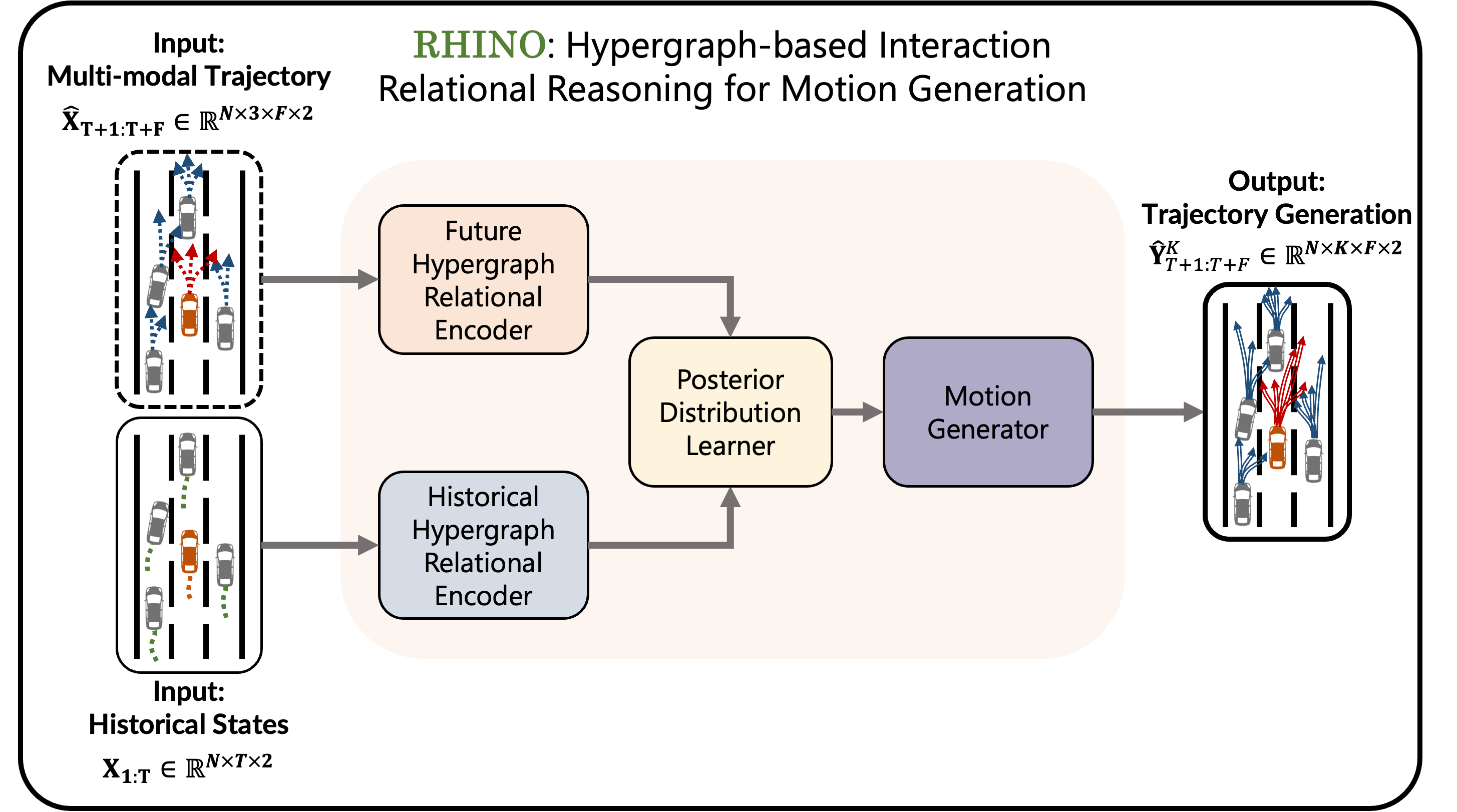
Thus, as illustrated in Figure 7, RHINO comprises the following modules:
-
1.
Hypergraph Relational Encoder, which transforms both the original historical states and predicted multi-agent multi-modal trajectories into hypergraphs, modeling and reasoning the underlying relation between the vehicles.
-
2.
Posterior Distribution Learner, which captures the posterior distribution of the future trajectory given the historical states and the predicted multi-modal future motion states of all the vehicles in the vehicle group.
-
3.
Motion Generator, which decodes the embeddings by concurrently reconstructing the historical states and generating the future trajectories.
3.3.2 Hypergraph Relational Encoder
We employ two Hypergraph Relational Encoder modules: a Historical Hypergraph Relational Encoder for handling historical states and a Future Hypergraph Relational Encoder for predicted multi-agent multi-modal trajectories from GIRAFFE. For the Historical Hypergraph Relational Encoder, the input historical states form an Agent Hypergraph . For the Future Hypergraph Relational Encoder, the predicted multi-agent multi-modal trajectories form an Agent-Behavior Hypergraph , where each agent node is expanded into three lateral behavior nodes with corresponding predicted future states. Both modules share the same structure regardless of the input hypergraph types.
Multi-scale Hypergraph Topology Inference
To comprehensively model group-wise interactions in the hypergraphs at multiple scales, we infer a multi-scale hypergraph to reflect interactions in groups with various sizes. Let be a multi-scale hypergraph, and be a set of nodes. As shown in Figure 8, at any scale , has a hyperedge set representing group-wise relations with hyperedges. A larger indicates a larger scale of agent groups, while models the finest pair-wise agent connections. The topology of each is represented as an incidence matrix .

To understand and quantify the dynamic interactions between agents within a given system, we adopt trajectory embedding to distill the motion states of agents into a compact and informative representation. To infer a multi-scale hypergraph, we construct hyperedges by grouping agents that have highly correlated trajectories, whose correlations could be measured by mapping the trajectories as a high-dimensional feature vector. For the -th agent in the system, the trajectory embedding is denoted as . This embedding is a function of the agent’s motion states, defined over a temporal window extending from time 1 to time . The embedding function , which is a trainable MLP, is responsible for transforming the motion states into a vector , where is the dimensionality of the embedded space. Mathematically, the trajectory embedding is represented as:
| (15) |
The affinity between agents is represented by an affinity matrix , which contains the pairwise relational weights between all agents. The affinity matrix is defined as:
| (16) |
Each element is computed as the correlation between the trajectory embeddings of the -th and -th agents. The correlation is the normalized dot product of the two trajectory embeddings, expressed as:
| (17) |
Here, denotes the L2 norm. The relational weight measures the strength of association between the trajectories of the -th and -th agents, capturing the degree to which their behaviors are correlated. This enables the assessment of interaction patterns and can uncover underlying social or physical laws governing agent dynamics.
The formulation of a hypergraph necessitates the strategic formation of hyperedges that reflect the complex interaction between the nodes in the system. At the outset, the 0-th scale hypergraph is considered, where the construction is based on pair-wise connections. Each node establishes a link with another node that has the highest affinity score with it.
As the complexity of the system is scaled up, beginning at scale , the methodology shifts towards group-wise connections. This shift is based on the intuition that agents within a particular group should display strong mutual correlations, suggesting a propensity for concerted action. To implement this, a sequence of increasing group sizes is established. For every node, denoted by , the objective is to discern a group of agents that are highly correlated, ultimately leading to groups or hyperedges at each scale . The hyperedge associated with a node at a given scale is indicated by . The determination of the most correlated agents is framed as an optimization problem, aiming to link these agents into a hyperedge that accounts for group dynamics:
| (18) |
| (19) |
The culmination of this hierarchical structuring is a multi-scale hypergraph, encapsulated by the set , where each scale embodies a distinct layer of abstraction in the representation of node relationships within the hypergraph.
Hypergraph Neural Message Passing
In order to discern the patterns of agent motion states from the inferred multi-scale hypergraph, we have tailored a multi-scale hypergraph neural message passing technique to construct the hypergraph topology. This method iteratively acquires the embeddings of vehicles and the corresponding interactions through node-to-hyperedge and hyperedge-to-node processes, as depicted in Figure 9.

The node-to-hyperedge mapping aggregates agent embeddings to generate interaction embeddings. Initially, for any given scale, the initial embedding for the th agent, . Each node is associated with a hyperedge , given that is an element of . This mapping facilitates the definition of the hyperedge interaction embedding. The hyperedge interaction embedding for a hyperedge is defined as a function of the embeddings of the nodes contained within it, modulated by the neural interaction strength and categorized through coefficients . The per-category function models the interaction process for each category, which is crucial for capturing the nuances of different interaction types. Each is a trainable MLP, responsible for processing the aggregated node embeddings within the context of a specific interaction category. The mathematical formulation is:
| (20) |
The neural interaction strength encapsulates the intensity of the interaction within the hyperedge and is obtained through a trainable model , applied to a collective embedding with a sigmoid function as Eq.(21). This collective embedding is represented as the weighted sum of the individual node embeddings within the hyperedge, signifying the aggregated information of agents in a group as Eq. (22). The weight for each node is determined by a trainable MLP as Eq.23.
| (21) |
| (22) |
| (23) |
The neural interaction category coefficient represent the model’s reasoning about which type of the interaction is likely for hyperedge , where denotes the probability of the -th neural interaction category within possible categories. These coefficients are computed using a softmax function applied to the output of another trainable MLP , which is further adjusted by an i.i.d. sample Gumbel distribution as described in C. which add some random noise and a temperature parameter which controlls the smoothness of probability distribution [45]:
| (24) |
These components, including neural interaction strength, interaction category coefficients, and per-category functions, provide a comprehensive mechanism for reasoning over complex, higher-order relationships, allowing the model to adapt its understanding of how agents collectively behave in diverse scenarios.
The process of hyperedge-to-node mapping is a pivotal step that allows for the update and refinement of agent embeddings within the hypergraph framework. Each hyperedge is mapped back onto its constituent nodes , assuming every is included in . The primary objective of this phase is to update the embedding of an agent. This is achieved through the function , which is a trainable MLP. The updated agent embedding is the result of the function applied to the concatenation of the agent’s current embedding and the sum of the embeddings of all hyperedges that the agent is part of. Formally, the update rule for the agent embedding is represented as:
| (25) |
where denotes the set of hyperedges associated with the -th node , and symbolize the operation of embedding concatenation. This operation fuses the individual node embedding with the collective information conveyed by the associated hyperedges. This amalgamation is crucial as it encapsulates the influence exerted by the interactions within the hyperedges onto the individual agent.
The Hypergraph Relational Encoder applies the node-to-hyperedge and hyperedge-to-node phases iteratively, allowing agent embeddings to be refined and enriched as relationships within hyperedges evolve. Upon the completion of these iterations, the output is constructed as the concatenation of the agent embeddings across all scales. The final agent embedding matrix is composed of the embeddings of all agents, where each agent embedding is a concatenation of the embeddings from all scales, expressed as:
| (26) |
where
| (27) |
3.3.3 Posterior Distribution Learner

In our study, we incorporated multi-scale hypergraph embeddings into a multi-agent trajectory generation system using the CVAE framework [46] to address the stochastic nature of each agent’s behavior, as shown in Figure 10. Here, we denote the historical trajectories as , and denote the predicted future trajectories as . Let denote the log-likelihood of predicted future trajectories given historical trajectories . The corresponding Evidence Lower Bound (ELBO) is defined as follows:
| (28) |
where represents the latent codes corresponding to all agents; is the conditional prior of , modeled as a Gaussian distribution. KL represents the Kullback–Leibler divergence function. In this framework, is implemented through an encoding process for embedding learning, and is realized via a decoding process that forecasts the future trajectories .
Thus, the goal of the Posterior Distribution Learner is to derive the Gaussian parameters for the approximate posterior distribution. This involves computing the mean and the variance based on the final output embeddings and the target embeddings . These parameters are generated through two separate trainable MLPs, and , respectively. The latent code , representing possible trajectories, is then sampled from a Gaussian distribution parameterized by these means and variances. The final output embeddings are a concatenation of the latent code , the final output embeddings , and the target embeddings . The equations governing these processes are as follows:
| (29) |
| (30) |
| (31) |
| (32) |
In these notations, and represent the mean and variance of the approximated posterior distribution. and are the trainable MLPs that produce these parameters. denotes the latent code of possible trajectories, and stands for the output embeddings, which fuses the latent code and the historical embeddings.
3.3.4 Motion Generator

The Motion Generator’s objective is dual: to predict future trajectories and to reconstruct past trajectories from the given embeddings. The decoder accomplishes this by applying successive processing blocks, each contributing a residual that refines the trajectory estimates, as shown in Figure 11. The first processing block, , takes the output embeddings and the target past trajectory to generate initial estimates of the future and reconstructed past trajectories and respectively.
| (33) |
Subsequently, the second block, , refines these estimates by considering the output embeddings and the residual of the past trajectory, which is the difference between the target past trajectory and the initial reconstructed past trajectory . This results in the second set of residuals and :
| (34) |
Both and are composed of a GRU encoder for sequence encoding and two MLPs serving as the output header. The final predicted future trajectory and the reconstructed past trajectory are obtained by summing the respective residuals from both processing blocks:
| (35) |
| (36) |
This approach enables the model to iteratively refine its predictions and reconstructions, leveraging the capability of deep learning models to capture complex patterns in the data through a series of non-linear transformations.
4 Experiments and Results
4.1 Data Preparations
This research leverages two open-source datasets for the purpose of model training and validation: the Next Generation Simulation (NGSIM) dataset [47],[48] and the HighD dataset [49]. The NGSIM dataset provides a comprehensive collection of vehicle trajectory data, capturing activity from the eastbound I-80 in the San Francisco Bay area and the southbound US 101 in Los Angeles. This dataset encapsulates real-world highway scenarios through overhead camera recordings at a sampling rate of 10Hz. The HighD dataset originates from aerial drone recordings executed at a 25 Hz frequency between 2017 and 2018 in the vicinity of Cologne, Germany. Spanning approximately 420 meters of bidirectional roadways, it records the movements of approximately 110,000 vehicles, encompassing both cars and trucks, traversing an aggregate distance of 45,000 km. After data pre-processing, the NGSIM dataset encompasses 662 thousand rows of data, capturing 1,380 individual trajectories, while the HighD dataset comprises 1.09 million data entries, including 3,913 individual trajectories. For the purpose of training and evaluation of the model, the partition of the data allocates to the training set and to the test set. For the temporal parameters of the model, we adopt frames to represent the historical horizon and frames to signify the prediction horizon.
4.2 Training and Evaluation Metrics
Training loss of GIRAFFE
The training loss function for GIRAFFE is a summation of three terms:
| (37) |
The first component, , is the mean squared error (MSE) between the fused predicted trajectory and the ground truth future trajectory:
| (38) |
The second component represents the negative log-likelihood (NLL) of the predicted driving intentions, treating it as a classification task:
| (39) |
The third component is the loss associated with the inference of the future-guided graph feature matrix, which is an intermediate output:
| (40) |
Training loss of RHINO
The training loss function for RHINO is also a summation of three components:
| (41) |
The first component, , corresponds to the ELBO loss [46] commonly used in variational autoencoders. It consists of a reconstruction loss term and a regularization term based on the Kullback-Leibler divergence between the learned distribution and a prior distribution:
| (42) |
The second component, , represents the Historical Trajectory Reconstruction loss, which measures how accurately the reconstructed historical trajectories match the true historical data:
| (43) |
The final component, , is the Variety loss, inspired by Social-GAN [21]. This loss encourages diversity in the predicted future trajectories by minimizing the error across multiple sampled future trajectories:
| (44) |
Table 1 presents the hyperparameter configurations used for the network architecture and the training process in the proposed framework.
| Parameter | Value | Parameter | Value |
|---|---|---|---|
| 30 | decaying factor | 0.6 | |
| 50 | 1 | ||
| neuron # of MLPs | 128 | 0.8 | |
| learning rate | 0.001 | 0.5 |
Evaluation metrics To ascertain the predictive accuracy of the model, we employ the Root Mean Square Error (RMSE) as the evaluative criterion. This metric quantitatively measures the deviation between the predicted position, expressed as , and the ground truth position, indicated by for all time step within the predictive horizon prediction horizon .
| (45) |
where the superscript denotes the -th test sample from the aggregate test sample set with length .
4.3 Results of Trajectory Generation
The experimental results for trajectory generation of the trajectories using the HighD dataset are presented in Figure 12. As can be found that, RHINO demonstrates strong generative capabilities, effectively producing plausible motion in a dynamic interactive traffic environment. To provide a more quantitative analysis, trajectory generation inaccuracies are illustrated in Figure 13. The generated longitudinal and lateral trajectories, along with the error box plots and heatmaps, are displayed. The box plot reveals that errors in both axes increase with the prediction time step by the natural of error propagation. However, the errors remain within an acceptable range, indicating decent model performance, which demonstrates high precision in trajectory generation. Notably, the model maintains a lower error margin for shorter prediction horizons, which is critical for short-term planning and reactive maneuvers in dynamic traffic environment.


The experiment focused on predicting vehicle trajectories within mixed traffic environments on highways by employing hypergraph inference to model group-based interactions. Through the application of hypergraph models at varying scales , the experiment captured the evolution of multi-vehicle interactions across both historical and future horizons. The figures depict these dynamics through three distinct columns: the first column presents vehicle trajectories and the corresponding hyperedges, visualized as polygons that encapsulate groups of interacting vehicles. The second column illustrates the affinity matrix, where both rows and columns represent vehicles, and the strength of their relationships is indicated by the matrix values. The third column shows the incidence matrix, detailing the relationship between nodes and hyperedges, with each column representing a hyperedge and each vehicle’s involvement in that hyperedge marked by a 1 in the corresponding row.
The hypergraph-based approach is particularly effective in modeling complex, higher-order interactions that are beyond the scope of traditional pairwise models. By forming hyperedges that encompass multiple vehicles, the model captures the collective influence that a group’s behavior exerts on an individual vehicle. For instance, in the scenario shown in Figure 14, at scale , when the target vehicle TAR initiates a lane change, the hypergraph reflects the interaction not only with a single neighboring vehicle but also with multiple surrounding vehicles, such as following vehicle F, preceding vehicle P, and preceding vehicle RP in the right lane. More examples are illustrated in A. This capability to model group-wise interactions across different scales is essential for accurately predicting vehicle trajectories in congested highway environments, where the actions of one vehicle can trigger ripple effects that influence an entire group. The hypergraph’s dynamic formation of hyperedges ensures that predicted trajectories remain adaptable and responsive to broader traffic conditions.
4.4 Comparisons and Ablation Study
To evaluate the privileges of our proposed method, the state of art methods (i.e., Social-LSTM (S-LSTM) [20], Convolutional Social-LSTM (CS-LSTM) [31], Planning-informed prediction (PiP) [50], Graph-based Interaction-aware Trajectory Prediction (GRIP) [26], Spatial-temporal dynamic attention network (STDAN) [22] are compared.
The compared results presented in Table 2 and Figure 15. As can be found that, the proposed framework demonstrates good performance with respect to the RMSE across a prediction horizon of 50 frames when compared with existing baseline models. It exhibits a reduced loss in comparison to C-LSTM, CS-LSTM, PiP, and GRIP. These outcomes suggest that the proposed model effectively captures salient features pertinent to long-term predictions. In summary, the proposed framework outperforms baseline models on the HighD dataset and delivers commendable performance on the NGSIM dataset.
Since the RHINO adopts the GIRAFFE, we further compare the trajectory generation capability of RHINO with our previous work [25] and its enhanced version GIRAFFE. Both RHINO model and the enhanced GIRAFFE model consistently outperform the baseline models, demonstrating superior performance in various metrics. This suggests that our proposed approaches effectively address the limitations present in prevailing models by robustly capturing complex interactions.
| Dataset | Horizon (Frame) | S-LSTM | CS-LSTM | PiP | GRIP | STDAN | GIRAFFE | RHINO |
|---|---|---|---|---|---|---|---|---|
| NGSIM | 10 | 0.65 | 0.61 | 0.55 | 0.37 | 0.42 | 0.38 | 0.32 |
| 20 | 1.31 | 1.27 | 1.18 | 0.86 | 1.01 | 0.89 | 0.78 | |
| 30 | 2.16 | 2.08 | 1.94 | 1.45 | 1.69 | 1.45 | 1.34 | |
| 40 | 3.25 | 3.10 | 2.88 | 2.21 | 2.56 | 2.46 | 2.17 | |
| 50 | 4.55 | 4.37 | 4.04 | 3.16 | 3.67 | 3.24 | 2.97 | |
| HighD | 10 | 0.22 | 0.22 | 0.17 | 0.29 | 0.19 | 0.19 | 0.19 |
| 20 | 0.62 | 0.61 | 0.52 | 0.68 | 0.27 | 0.42 | 0.26 | |
| 30 | 1.27 | 1.24 | 1.05 | 1.17 | 0.48 | 0.81 | 0.42 | |
| 40 | 2.15 | 2.10 | 1.76 | 1.88 | 0.91 | 1.13 | 0.65 | |
| 50 | 3.41 | 3.27 | 2.63 | 2.76 | 1.66 | 1.56 | 0.89 |

Ablation study is conducted to provide more insights into the performance of our RHINO model, especially the impact of different components on the prediction performance by disabling the corresponding component from the entire RHINO. In particular, we consider the following four variants:
-
1.
RHINO w/o HG (hypergraph) variant does not use the multi-scale hypergraphs representation but only adopts the pair-wise connected graph representations in the Hypergraph Relational Encoder.
-
2.
RHINO w/o MM (multi-modal) variant does not adopt the multi-agent multi-modal trajectory prediction results and only use the single predicted future states for each agent as the input of the RHINO.
-
3.
RHINO w/o PDL (posterior distribution learner) variant skips the Posterior Distribution Learner and directly input the graph embedding into the Motion Generator.
| Horizon (Frame) | RHINO w/o HG | RHINO w/o MM | RHINO w/o PDL | RHINO |
|---|---|---|---|---|
| 10 | 0.21 | 0.22 | 0.24 | 0.19 |
| 20 | 0.31 | 0.37 | 0.42 | 0.26 |
| 30 | 0.68 | 0.73 | 0.80 | 0.42 |
| 40 | 0.97 | 1.06 | 1.18 | 0.65 |
| 50 | 1.25 | 1.34 | 1.57 | 0.89 |

An investigation into the effects of model design variations, as presented in Table 3 and Figure 16. The removal of various components from RHINO invariably leads to performance degradation to varying degrees. Compared to the full RHINO, omitting the multi-scale hypergraphs results in an evident increase in prediction error across the prediction horizon, indicating that modeling and reasoning group-wise interactions using hypergraphs, rather than solely pair-wise interactions, enhances prediction accuracy which underscores the necessity of hypergraphs. Further, excluding the multi-agent multi-modal trajectory prediction input leads to a more substantial degradation in performance, highlighting the importance of incorporating multi-modal motion states and discussing the corresponding group-wise interactions among multiple driving behaviors of multiple agents. Lastly, the absence of the Posterior Distribution Learner module emphasizes its critical role in handling the stochasticity of each agent’s behavior. All these experiments justify the effectiveness of the full model.
5 Conclusions
In this study, we proposed a hypergraph enabled multi-modal probabilistic motion prediction framework with reasonings. This framework consists of two main components: GIRAFFE and RHINO. GIRAFFE focuses on predicting the interactive vehicular trajectories considering modalities. Based on that, RHINO, leveraging the flexibility and strengths on modeling the group-wise interactions, facilitate relational reasoning among vehicles and multi-modalities to render plausible vehicles trajectories. The framework extends traditional interaction models by introducing an agent-behavior hypergraph. This approach better aligns with traffic physics while being grounded in the mathematical rigor of hypergraph theory. Further, the approach employs representation learning to enable explicit interaction relational reasoning. This involves considering future relations and interactions and learning the posterior distribution to handle the stochasticity of behavior for each vehicle. As a result, the framework excels in capturing high-dimensional, group-wise interactions across various behavioral modalities.
The framework is tested using the NGSIM and HighD datasets. The results show that the proposed framework effectively models the interactions among groups of vehicles and their corresponding multi-modal behaviors. Comparative studies demonstrate that the framework outperforms prevailing algorithms in prediction accuracy. To further validate the effectiveness of each component, ablation studies were conducted, revealing that the full model performs best.
Several potential extensions of the framework include incorporating road geometries, vehicle types, and real-time weather data to improve trajectory prediction. By integrating weather information from sources like the OpenWeather API, the system could adjust predictions based on conditions such as temperature, wind, and precipitation, enhancing safety and route optimization [51]. Additional enhancements, like traffic signal integration, V2V and V2I communication, and human driver intent, could further improve accuracy and reliability in dynamic urban environments, minimizing disruptions and fostering safer, more informed autonomous driving.
Acknowledgement:
This research is funded by Federal Highway Administration (FHWA) Exploratory Advanced Research 693JJ323C000010. The results do not reflect FHWA’s opinions.
References
- [1] Gao, J., Sun, C., Zhao, H., Shen, Y., Anguelov, D., Li, C. & Schmid, C. Vectornet: Encoding hd maps and agent dynamics from vectorized representation. Proceedings Of The IEEE/CVF Conference On Computer Vision And Pattern Recognition. pp. 11525-11533 (2020)
- [2] Li, S., Wang, Z., Zheng, Y., Sun, Q., Gao, J., Ma, F. & Li, K. Synchronous and asynchronous parallel computation for large-scale optimal control of connected vehicles. Transportation Research Part C: Emerging Technologies. 121 pp. 102842 (2020)
- [3] Shi, H., Zhou, Y., Wu, K., Wang, X., Lin, Y. & Ran, B. Connected automated vehicle cooperative control with a deep reinforcement learning approach in a mixed traffic environment. Transportation Research Part C: Emerging Technologies. 133 pp. 103421 (2021), https://www.sciencedirect.com/science/article/pii/S0968090X21004150
- [4] Shi, H., Zhou, Y., Wu, K., Chen, S., Ran, B. & Nie, Q. Physics-informed deep reinforcement learning-based integrated two-dimensional car-following control strategy for connected automated vehicles. Knowledge-Based Systems. 269 pp. 110485 (2023)
- [5] Zhou, D., Hang, P. & Sun, J. Reasoning graph-based reinforcement learning to cooperate mixed connected and autonomous traffic at unsignalized intersections. Transportation Research Part C: Emerging Technologies. 167 pp. 104807 (2024)
- [6] Liu, H., Wu, K., Fu, S., Shi, H. & Xu, H. Predictive analysis of vehicular lane changes: An integrated lstm approach. Applied Sciences. 13, 10157 (2023)
- [7] Suo, S., Regalado, S., Casas, S. & Urtasun, R. Trafficsim: Learning to simulate realistic multi-agent behaviors. Proceedings Of The IEEE/CVF Conference On Computer Vision And Pattern Recognition. pp. 10400-10409 (2021)
- [8] Deo, N. & Trivedi, M. Multi-modal trajectory prediction of surrounding vehicles with maneuver based lstms. 2018 IEEE Intelligent Vehicles Symposium (IV). pp. 1179-1184 (2018)
- [9] Wang, H., Meng, Q., Chen, S. & Zhang, X. Competitive and cooperative behaviour analysis of connected and autonomous vehicles across unsignalised intersections: A game-theoretic approach. Transportation Research Part B: Methodological. 149 pp. 322-346 (2021)
- [10] Trentin, V., Artuñedo, A., Godoy, J. & Villagra, J. Multi-modal interaction-aware motion prediction at unsignalized intersections. IEEE Transactions On Intelligent Vehicles. (2023)
- [11] Ali, Y., Bliemer, M., Zheng, Z. & Haque, M. Cooperate or not? Exploring drivers’ interactions and response times to a lane-changing request in a connected environment. Transportation Research Part C: Emerging Technologies. 120 pp. 102816 (2020)
- [12] Karle, P., Geisslinger, M., Betz, J. & Lienkamp, M. Scenario understanding and motion prediction for autonomous vehicles—review and comparison. IEEE Transactions On Intelligent Transportation Systems. 23, 16962-16982 (2022)
- [13] Li, G., Jiang, B., Zhu, H., Che, Z. & Liu, Y. Generative attention networks for multi-agent behavioral modeling. Proceedings Of The AAAI Conference On Artificial Intelligence. 34, 7195-7202 (2020)
- [14] Han, Z., Fink, O. & Kammer, D. Collective relational inference for learning heterogeneous interactions. Nature Communications. 15, 3191 (2024)
- [15] Zhong, X., Zhou, Y., Ahn, S. & Chen, D. Understanding heterogeneity of automated vehicles and its traffic-level impact: A stochastic behavioral perspective. Transportation Research Part C: Emerging Technologies. 164 pp. 104667 (2024)
- [16] Kipf, T., Fetaya, E., Wang, K., Welling, M. & Zemel, R. Neural relational inference for interacting systems. International Conference On Machine Learning. pp. 2688-2697 (2018)
- [17] Li, J., Yang, F., Tomizuka, M. & Choi, C. Evolvegraph: Multi-agent trajectory prediction with dynamic relational reasoning. Advances In Neural Information Processing Systems. 33 pp. 19783-19794 (2020)
- [18] Xu, C., Wei, Y., Tang, B., Yin, S., Zhang, Y., Chen, S. & Wang, Y. Dynamic-group-aware networks for multi-agent trajectory prediction with relational reasoning. Neural Networks. 170 pp. 564-577 (2024)
- [19] Park, D., Ryu, H., Yang, Y., Cho, J., Kim, J. & Yoon, K. Leveraging future relationship reasoning for vehicle trajectory prediction. ArXiv Preprint ArXiv:2305.14715. (2023)
- [20] Alahi, A., Goel, K., Ramanathan, V., Robicquet, A., Fei-Fei, L. & Savarese, S. Social lstm: Human trajectory prediction in crowded spaces. Proceedings Of The IEEE Conference On Computer Vision And Pattern Recognition. pp. 961-971 (2016)
- [21] Gupta, A., Johnson, J., Fei-Fei, L., Savarese, S. & Alahi, A. Social gan: Socially acceptable trajectories with generative adversarial networks. Proceedings Of The IEEE Conference On Computer Vision And Pattern Recognition. pp. 2255-2264 (2018)
- [22] Chen, X., Zhang, H., Zhao, F., Hu, Y., Tan, C. & Yang, J. Intention-aware vehicle trajectory prediction based on spatial-temporal dynamic attention network for internet of vehicles. IEEE Transactions On Intelligent Transportation Systems. 23, 19471-19483 (2022)
- [23] Zhang, K., Zhao, L., Dong, C., Wu, L. & Zheng, L. AI-TP: Attention-based interaction-aware trajectory prediction for autonomous driving. IEEE Transactions On Intelligent Vehicles. 8, 73-83 (2022)
- [24] Kim, H., Kim, D., Kim, G., Cho, J. & Huh, K. Multi-head attention based probabilistic vehicle trajectory prediction. 2020 IEEE Intelligent Vehicles Symposium (IV). pp. 1720-1725 (2020)
- [25] Wu, K., Zhou, Y., Shi, H., Li, X. & Ran, B. Graph-Based Interaction-Aware Multimodal 2D Vehicle Trajectory Prediction Using Diffusion Graph Convolutional Networks. IEEE Transactions On Intelligent Vehicles. 9, 3630-3643 (2024)
- [26] Li, X., Ying, X. & Chuah, M. Grip: Graph-based interaction-aware trajectory prediction. 2019 IEEE Intelligent Transportation Systems Conference (ITSC). pp. 3960-3966 (2019)
- [27] Zhou, H., Ren, D., Xia, H., Fan, M., Yang, X. & Huang, H. Ast-gnn: An attention-based spatio-temporal graph neural network for interaction-aware pedestrian trajectory prediction. Neurocomputing. 445 pp. 298-308 (2021)
- [28] Huang, Y., Bi, H., Li, Z., Mao, T. & Wang, Z. Stgat: Modeling spatial-temporal interactions for human trajectory prediction. Proceedings Of The IEEE/CVF International Conference On Computer Vision. pp. 6272-6281 (2019)
- [29] Amirian, J., Hayet, J. & Pettré, J. Social ways: Learning multi-modal distributions of pedestrian trajectories with gans. Proceedings Of The IEEE/CVF Conference On Computer Vision And Pattern Recognition Workshops. pp. 0-0 (2019)
- [30] Khandelwal, S., Qi, W., Singh, J., Hartnett, A. & Ramanan, D. What-if motion prediction for autonomous driving. ArXiv Preprint ArXiv:2008.10587. (2020)
- [31] Deo, N. & Trivedi, M. Convolutional social pooling for vehicle trajectory prediction. Proceedings Of The IEEE Conference On Computer Vision And Pattern Recognition Workshops. pp. 1468-1476 (2018)
- [32] Messaoud, K., Yahiaoui, I., Verroust-Blondet, A. & Nashashibi, F. Attention based vehicle trajectory prediction. IEEE Transactions On Intelligent Vehicles. 6, 175-185 (2020)
- [33] Feng, X., Cen, Z., Hu, J. & Zhang, Y. Vehicle trajectory prediction using intention-based conditional variational autoencoder. 2019 IEEE Intelligent Transportation Systems Conference (ITSC). pp. 3514-3519 (2019)
- [34] Wang, Y., Zhao, S., Zhang, R., Cheng, X. & Yang, L. Multi-vehicle collaborative learning for trajectory prediction with spatio-temporal tensor fusion. IEEE Transactions On Intelligent Transportation Systems. 23, 236-248 (2020)
- [35] Zhou, Y., Zhong, X., Chen, Q., Ahn, S., Jiang, J. & Jafarsalehi, G. Data-driven analysis for disturbance amplification in car-following behavior of automated vehicles. Transportation Research Part B: Methodological. 174 pp. 102768 (2023)
- [36] Huang, Z., Wu, J. & Lv, C. Driving behavior modeling using naturalistic human driving data with inverse reinforcement learning. IEEE Transactions On Intelligent Transportation Systems. 23, 10239-10251 (2021)
- [37] Sheng, Z., Xu, Y., Xue, S. & Li, D. Graph-based spatial-temporal convolutional network for vehicle trajectory prediction in autonomous driving. IEEE Transactions On Intelligent Transportation Systems. 23, 17654-17665 (2022)
- [38] Gao, Y., Zhang, Z., Lin, H., Zhao, X., Du, S. & Zou, C. Hypergraph learning: Methods and practices. IEEE Transactions On Pattern Analysis And Machine Intelligence. 44, 2548-2566 (2020)
- [39] Feng, Y., You, H., Zhang, Z., Ji, R. & Gao, Y. Hypergraph neural networks. Proceedings Of The AAAI Conference On Artificial Intelligence. 33, 3558-3565 (2019)
- [40] Zhou, R., Zhou, H., Gao, H., Tomizuka, M., Li, J. & Xu, Z. Grouptron: Dynamic multi-scale graph convolutional networks for group-aware dense crowd trajectory forecasting. 2022 International Conference On Robotics And Automation (ICRA). pp. 805-811 (2022)
- [41] Xu, C., Li, M., Ni, Z., Zhang, Y. & Chen, S. Groupnet: Multiscale hypergraph neural networks for trajectory prediction with relational reasoning. Proceedings Of The IEEE/CVF Conference On Computer Vision And Pattern Recognition. pp. 6498-6507 (2022)
- [42] Li, J., Hua, C., Ma, H., Park, J., Dax, V. & Kochenderfer, M. Multi-Agent Dynamic Relational Reasoning for Social Robot Navigation. ArXiv Preprint ArXiv:2401.12275. (2024)
- [43] Wu, Y., Zhuang, D., Labbe, A. & Sun, L. Inductive graph neural networks for spatiotemporal kriging. Proceedings Of The AAAI Conference On Artificial Intelligence. 35, 4478-4485 (2021)
- [44] Li, Y., Yu, R., Shahabi, C. & Liu, Y. Diffusion convolutional recurrent neural network: Data-driven traffic forecasting. ArXiv Preprint ArXiv:1707.01926. (2017)
- [45] Jang, E., Gu, S. & Poole, B. Categorical reparameterization with gumbel-softmax. ArXiv Preprint ArXiv:1611.01144. (2016)
- [46] Pagnoni, A., Liu, K. & Li, S. Conditional variational autoencoder for neural machine translation. ArXiv Preprint ArXiv:1812.04405. (2018)
- [47] J. Colyar and J. Halkias, “U.S. Highway 101 dataset,” 2007.
- [48] J. Colyar and J. Halkias, “U.S. Highway 80 dataset,” 2006.
- [49] R. Krajewski, J. Bock, L. Kloeker, and L. Eckstein, “The highD Dataset: A Drone Dataset of Naturalistic Vehicle Trajectories on German Highways for Validation of Highly Automated Driving Systems,” in IEEE Conference on Intelligent Transportation Systems, Proceedings, ITSC, 2018, vol. 2018-November. doi: 10.1109/ITSC.2018.8569552.
- [50] Song, H., Ding, W., Chen, Y., Shen, S., Wang, M. & Chen, Q. Pip: Planning-informed trajectory prediction for autonomous driving. Computer Vision–ECCV 2020: 16th European Conference, Glasgow, UK, August 23–28, 2020, Proceedings, Part XXI 16. pp. 598-614 (2020)
- [51] Ye, X., Li, S., Das, S. & Du, J. Enhancing routes selection with real-time weather data integration in spatial decision support systems. Spatial Information Research. 32, 373-381 (2024)
Appendix A Experiment results of trajectory generation with hypergraph inference

In Scenario 2, at scale (Figure 17), the target vehicle TAR forms a strong historical interaction with multiple vehicles, including the preceding vehicle P, preceding vehicle LP in the left lane, and following vehicles LF and F in the left lane. However, in the future states, vehicle LF exits the interaction group, while the preceding vehicle RP in the left lane joins the group as the target vehicle accelerates toward RF.

In Scenario 3, at scale (Figure 18), the target vehicle TAR forms a weak historical interaction with the preceding vehicles P and LP in the left lane. As traffic conditions change over time, these interactions strengthen in the future, highlighting the need to account for dynamic shifts when predicting future states, as historical data alone may not capture the evolving complexity of vehicle interactions. These findings emphasize the importance of adaptive models in predicting multi-agent traffic dynamics.
Appendix B Diffusion Graph Convolutional Networks (DGCN)
The Diffusion Graph Convolutional Networks (DGCN) module models bidirectional dependencies between nodes in the graph embedding, following [43, 44]. The DGCN layer, denoted , applies diffusion convolution to the graph signal in both forward and reverse directions:
| (46) |
In this equation, represents the output of the -th layer, with the input to the first layer being the masked feature matrix . The forward transition matrix captures downstream node dependencies, while the backward transition matrix captures upstream dependencies. The function represents a Chebyshev polynomial used to approximate convolution with the -th order neighbors of each node. This is expressed as . Learnable parameters and assign weights to input data in the -th layer. The forward diffusion process captures the influence of surrounding vehicles on a given vehicle, while the reverse diffusion process models the influence that the vehicle transmits to its surroundings.
Appendix C Gumbel Softmax Distribution
The Gumbel-Softmax distribution [45] provides a differentiable approximation of the categorical distribution, crucial for neural networks that rely on gradient-based optimization. Traditional categorical sampling, involving non-differentiable operations like argmax, poses challenges for backpropagation. Gumbel-Softmax addresses this by replacing argmax with a differentiable softmax function, allowing gradients to flow during training. Based on the Gumbel-Max trick, which adds Gumbel noise to log-probabilities followed by argmax, the Gumbel-Softmax substitutes softmax to maintain differentiability. The formula of the sample vectors is:
| (47) |
Here, are categorical probabilities, is Gumbel noise, and controls the distribution’s sharpness. As approaches zero, the Gumbel-Softmax approximates a one-hot distribution. Larger values result in a smoother distribution, useful for early training exploration. This property makes Gumbel-Softmax valuable for tasks like variational autoencoders and reinforcement learning, where discrete sampling with differentiability is needed.