Hydroelastic lumps in shallow water
Abstract
Hydroelastic solitary waves propagating on the surface of a three-dimensional ideal fluid through the deformation of an elastic sheet are studied. The problem is investigated based on a Benney-Luke-type equation derived via an explicit non-local formulation of the classic water wave problem. The normal form analysis is carried out for the newly developed equation, which results in the Benney-Roskes-Davey-Stewartson (BRDS) system governing the coupled evolution of the envelope of a carrier wave and the wave-induced mean flow. Numerical results show three types of free solitary waves in the Benney-Luke-type equation: plane solitary wave, lump (i.e., fully localized traveling waves in three dimensions), and transversally periodic solitary wave, and they are counterparts of the BRDS solutions. They are linked together by a dimension-breaking bifurcation where plane solitary waves and lumps can be viewed as two limiting cases, and transversally periodic solitary waves serve as intermediate states. The stability and interaction of solitary waves are investigated via a numerical time integration of the Benney-Luke-type equation. For a localized load moving on the elastic sheet with a constant speed, it is found that there exists a transcritical regime of forcing speed for which there are no steady solutions. Instead, periodic shedding of lumps can be observed if the forcing moves at speed in this range.
Keywords: hydroelastic wave; lump; free-surface flow
1 Introduction
Vibrations of a thin elastic plate on top of a fluid body due to gravity, elasticity, and external load are known as hydroelastic waves or flexural-gravity (FG) waves. Hydroelastic waves have wide applications in the safe use of floating ice covers as transport links and the construction of very large floating platforms. Typical lengths of hydroelastic waves are generally from tens to hundreds of meters, and then these waves are easily observed in field campaigns. Two famous field studies on hydroelastic waves were conducted respectively in McMurdo Sound near Antarctica for the case of deep water [1] and Lake Saroma in Japan for shallow water [2]. Recently, Van der Sanden and Short [3] measured the ice deflection induced by the motion of a vehicle based on the satellite synthetic-aperture radar.
In the past few decades, many analytical and numerical studies of hydroelastic waves concentrated on the two-dimensional (2D) problem. The Euler-Bernoulli beam theory was extensively used in early works, which is a good approximation for small-amplitude deformations of the elastic sheet. However, this theory is not so suitable when the deformation becomes large. Therefore, the nonlinear Kirchhoff-Love (KL) plate theory was later developed for describing large-amplitude deformations. There have been rich studies based on this nonlinear elastic model. Părău and Dias [4] derived the forced nonlinear Schrödinger (NLS) equation which predicted the existence of solitary waves if the fluid depth was in a specific range, and performed numerical computations of the full Euler equations for validation. Milewski et al. [5] considered hydroelastic waves in deep water via asymptotic and numerical methods for both forced and unforced problems. They found a transcritical range of load speed where the shedding of solitary waves occurred for large external forces in unsteady simulations. It is noted that in deep water, hydroelastic solitary waves exist only at finite amplitude, which is coincident with the defocusing nature of the NLS equation at the phase speed minimum. Milewski et al. [6] numerically found dark solitary waves in deep water in the full Euler equations using the conformal mapping technique, which were also predicted by the defocusing NLS equation.
Recently, Toland [7] proposed a new model for ice sheets based on the Cosserat theory of hydroelastic shells satisfying Kirchhoff’s hypotheses. The chief advantage of the Toland model over the KL model is that it conserves the elastic potential energy and hence has a clear variational structure. Guyenne and Părău [8] computed both depression and elevation solitary waves below the phase speed minimum in deep water based on this model. Their numerical results were complemented by Wang et al. [9], who found new highly nonlinear elevation solitary waves using a numerical continuation method. Gao et al. [10] discovered a new class of non-symmetric solitary waves arising via spontaneous symmetry-breaking bifurcations. Periodic and generalized hydroelastic solitary waves were explored extensively by Gao and Vanden-Broeck [11] using a series truncation method.
Linear models for both elasticity and fluid flow were used in early works of the three-dimensional (3D) problem, and hence the asymptotic Fourier analysis technique was applicable. Of note is the work of Davys et al. [12], who considered waves generated by a concentrated moving point load and obtained wave patterns, and Milinazzo et al. [13], who investigated the steady response of a uniform ice sheet induced by a rectangular moving load. Recently, Părău and Vanden-Broeck [14], Dinvay et al. [15] investigated various types of responses of a floating ice sheet of infinite extent for disturbances moving at different velocities considering the nonlinear effect of the flow. Milewski and Wang [16] derived a Benney-Roskes-Davey-Stewartson (BRDS) system in the small-amplitude modulational asymptotic limit, on the base of which they studied the bifurcation mechanism of lumps together with their stability properties for a range of depths. Free hydroelastic lumps were computed by Wang et al. [17] using a quintic truncation model in the Hamiltonian framework and by Trichtchenko et al. [18] based on a boundary integral equation method.
There are challenges to the 3D hydroelastic wave problem due to the complexity of the full Euler equations. Therefore, simplified equations in various asymptotic regimes are necessary for reducing model complexity and computational cost. Guyenne and Părău [19] derived a fifth-order Kadomtsev-Petviashvili (KP) equation in the long-wave approximation. It is noted that the KP equation was proposed for uni-directional surface waves with weak transverse variations. It cannot correctly describe the two-way propagation of surface waves, such as wave reflection/transmission across the media interface and head-on collisions of solitary waves. Additionally, it is not suitable to use an anisotropic model to study wave phenomena whose transverse variations are similar to those in the primary direction of propagation, such as the Kelvin wake and oblique interactions between lumps. Thus, though anisotropic uni-directional models have been successful in many aspects of free-surface problems, isotropic bi-directional models are still needed in some cases.
Without the elastic cover, the isotropic Benney-Luke equation was derived originally by Benney and Luke [20] to describe the bi-directional evolution of 3D small-amplitude pure gravity waves when the horizontal length scale is long compared with the fluid depth. Pego and Quintero [21] rigorously proved the existence of finite-energy solitary waves for the Benney-Luke equation, including the effect of surface tension. Berger and Milewski [22] established an explicit connection between the KP-I equation and the Benney-Luke equation considering strong surface tension, and studied the dynamics of lumps numerically. In many situations, the fluid depth is small compared with the typical wavelength of hydroelastic waves (e.g., see the experiment in Lake Saroma in Japan [2]). Therefore, to simplify the primitive equations, it is reasonable to use the long-wave approximation and extend the Benney-Luke equation to the hydroelastic wave problem.
The paper is structured as follows. In §2, the detailed derivations of the Benney-Luke-type model and the associated envelope equation are presented. We then discuss the results of the envelope equation that served as a theoretical underpinning for hydroelastic solitary waves. In §3, we numerically show different types of solitary waves in the Benney-Luke-type equation, together with their stability properties and collision dynamics. Besides, we compute the responses exerted by a locally confined load moving with a uniform speed, which features the shedding of lumps when the load speed is in the transcritical regime. A conclusion is given in §4.
2 Formulation
2.1 The Benney-Luke-type equation
We consider a three-dimensional incompressible and inviscid fluid of density covered by a deformable ice sheet of density and the thickness . The displacement of the ice cover is denoted by , where and are horizontal coordinates, and the -axis points upwards with the undisturbed ice sheet. The fluid is bounded below by a rigid bed located at , where is constant. The motion of the fluid is assumed to be irrotational; therefore, we can introduce velocity potential, , which satisfies the Laplace equation
| (1) |
At the free surface , the kinematic and dynamic boundary conditions read
| (2) |
and
| (3) |
where is the acceleration due to gravity, the restoring force due to elastic bending, and the external pressure exerted on the ice sheet (if , the pressure acts downwards). The pressure resulting from the linear elastic bending model takes the form
| (4) |
where is the flexural rigidity ( is Young’s modulus and is the Poisson ratio), and is the bi-Laplacian operator acting on horizontal variables. Hence the dynamic condition can be rewritten as
| (5) |
Finally, the impermeability boundary condition at the bottom,
| (6) |
completes the whole system.
Ablowitz et al. [23] introduced an explicit non-local formulation of the classical equations of water waves in both two and three dimensions. Following their work, we will derive a Benney-Luke-type equation for hydroelastic waves in the shallow-water regime in the subsequent analyses.
We reformulate these equations in terms of the surface displacement and surface velocity potential. If we denote by the value of at the free surface, then the dynamic boundary condition can be recast to
| (7) |
where is the horizontal gradient operator. For arbitrary harmonic functions and , it is straightforward to verify that
| (8) |
We choose , where is the magnitude of the wavenumber vector. Substituting this solution into Eq. (8), integrating over the space occupied by the fluid, and applying the divergence theorem, one obtains the global relation
| (9) | ||||
where is the outward unit normal vector of , the boundary of the fluid body, and is the surface element. Using the kinematic boundary condition at the free surface and the impermeability condition at the bottom, Eq. (9) can be recast to
| (10) |
In the same vein, substituting into Eq. (8) yields
| (11) |
Subtracting Eq. (11) from Eq. (10) gives
| (12) |
where we denote by the wavenumber vector.
It is convenient to non-dimensionalize the problem using the Boussinesq scaling to proceed with the derivation. In this respect, we introduce the typical wavelength , the small amplitude , and the shallow-water speed , and rescale the variables as
Then the dimensionless dynamic boundary condition and global relation read
| (13) |
and
| (14) |
respectively, where asterisks have been dropped for the ease of notations, and the dimensionless parameters read
Let and this assumption corresponds to , , , , and . It is noted that in the real situation, is usually much smaller than due to the smallness of ; however, it does not qualitatively change the model equation if we involve the inertia effect in the current problem.
We expand the dynamic condition (13) and the global relation (14) with respect to small parameters and retain terms valid up to to achieve a balance between dispersion and nonlinearity. After some algebra, one obtains the following Boussinesq-type equations
| (15) |
| (16) |
where is the horizontal Laplace operator, and Eq. (16) is obtained by taking the inverse Fourier transform. By combining Eqs. (15) and (16) to eliminate and , one arrives at
| (17) |
Upon noticing to leading order, Eq. (17) can be reformulated to
| (18) |
a Benney-Luke-type equation with a time-dependent external force.
By letting in Eq. (18), we can derive the fifth-order Kadomtsev-Petviashvili (KP) equation, a single evolution equation describing uni-directional waves with weak variations in the transverse direction. For this purpose, we seek a solution of the form , where , , and . In this asymptotic limit, we can rewrite Eq. (18) as
upon neglecting higher-order terms. Differentiating the above equation with respect to and substituting , we obtain the fifth-order KP equation
| (19) |
In the context of hydroelastic waves, the fifth-order KP equation (19) was first obtained by Hărăgus-Courcelle and Andrej [24] via a regular asymptotic expansion and re-derived by Guyenne and Părău [19] based on the Taylor expansion of the Dirichlet-Neumann operator in the Hamiltonian framework. If the -dependence is negligible, Eq. (19) reduces to the fifth-order Korteweg-de Vries equation, which is known as a reduced model for hydroelastic waves in channels (see [25] for more details).
Finally, we show that without the external forcing, Eq. (18) has a Hamiltonian structure with the Hamiltonian functional
| (20) |
The canonical variables are and , where is defined as
| (21) |
Calculating the variational derivatives with respect to the canonical variables gives
| (22) |
and
| (23) | ||||
2.2 The Benney-Roskes-Davey-Stewartson system
Traditionally, weakly nonlinear wavepacket dynamics are investigated using the cubic nonlinear Schrödinger (NLS) equation, which describes the envelope evolution of a monochromatic carrier wave in deep water. In the case of finite depth, the wave envelope is strongly coupled with the induced mean flow, and their interactions are governed by the Benney-Roskes-Davey-Stewartson (BRDS) system. It is well known that the envelope equations play a key role in understanding the existence of solitary wave solutions and their stability properties for both gravity-capillary and flexural-gravity problems (see [16, 26] for example). In the context of 3D hydroelastic waves in the shallow-water regime, we expect to gain some theoretical predictions from the BRDS system derived from Eq. (18) in the absence of external forcing. For this purpose, we expand the solution of Eq. (18) as
| (24) |
where the assumption of small amplitude is taken through the expansion in powers of . Then the equation to leading order reads
whose real solution is given by
| (25) |
where c.c. stands for complex conjugation, , and are slow variables, is the fast variable with the dispersion relation , and is a real slow-varying, mean term.
We substitute , , and into the Benney-Luke-type equation. At second order, one obtains
| (26) |
and solve for what remains, i.e., solve
with . The former equation implies that , where is called the group velocity defined as
The latter equation can be solved by letting , which gives
To obtain the BRDS system, we transform to a moving reference frame and denote by a much slower time scale. Then to the third order, we can get
| (27) |
| (28) |
where
The BRDS system (27)–(28) is valid for arbitrary ; however, in the current context, we focus on the case , where is the wavenumber corresponding to the phase speed minimum. Since , , and , the system is of ‘elliptic-elliptic’ type as the coefficients of , , , and are of the same sign. Following [27], the system’s behavior then depends on the sign of the parameter defined as
It was proved by Cipolatti [27] that is a sufficient condition for the BRDS system to have a localized ground state solution, and the system is therefore called ‘focussing’. For the case that transverse modulations are absent (i.e., ), the BRDS system (27)–(28) degenerates to the one-dimensional NLS equation . It is well known that the simplest solution to the one-dimensional focussing NLS equation takes an exact formula: with and .
In infinite depth, the effect of the mean flow vanishes, and the evolution is governed by the two-dimensional NLS equation
| (29) |
where coefficients have all been normalized to unity. It was shown by Alfimov et al. [28] that for the nonlinear eigenvalue problem of Eq. (29),
there exists a one-parameter family of solutions for , where represents the basic period in the -direction. In contrast to plane solitons, this new type of solution features a nontrivial variation in the transverse direction. As the basic period , the solution degenerates to the plane soliton solution, and hence the emergence of transversally periodic solitons is called a dimension-breaking bifurcation. Following the new branch by increasing the bifurcation parameter , a fully localized solution with circular symmetry can be obtained as ; that is to say, these new solutions are a bridge between plane solitons and lumps. Inspired by the results of the asymptotic model, Milewski and Wang [29] found transversally periodic solitary waves in the full gravity-capillary wave problem corresponding to its NLS counterpart. Additionally, these authors predicted that the threshold wavelength of transverse instability of a plane solitary wave coincides with the dimension-breaking bifurcation point.
Motivated by their work, we numerically explore various types of localized steady solutions to the BRDS system through the dimension-breaking bifurcation, which provide a solid underpinning for the existence of solitary waves in the Benney-Luke-type equation. Without loss of generality, we set , , , and as a result, the BRDS system is of focussing type since the coefficient . To find localized time harmonic solutions to the BRDS system, we assume , and then the steady BRDS system in the non-local form can be written as
| (30) |
where and . The parameter varying from 0 to 1 is introduced to assist with computing steady solutions to Eq. (30). The numerical process can be divided into three steps in general. First of all, by letting , the problem can be reduced to the steady focussing cubic NLS equation. This equation, after normalization, has countably many localized radial solutions (see [30] for example), but we focus only on computing the ground state solution. Secondly, the obtained ground state solution is taken as the initial guess, and the non-local term in Eq. (30) is included by using a numerical continuation in up to , resulting in a lump solution to the BRDS system. The lump is computed using the standard pseudo-spectral method in a horizontally double periodic domain with small wavenumbers and in the - and -direction, respectively. Finally, the dimension-breaking bifurcation curve can be obtained by using as the continuation parameter, and the interested readers are referred to [16] for more details on the numerical scheme.
By gradually increasing (equivalently, decreasing the basic period in the -direction), a one-parameter family of solutions for is obtained. As the basic period , degenerates to a plane soliton, while , a lump solution emerges. The intermediate states which bridge the two limiting cases correspond to transversally periodic solitons. Fig. 1 shows the typical wave profiles on this new branch: 1 and 1 are the two limiting cases, while 1 is the intermediate case. It is noted that the bifurcation wavenumber is closely related to the transverse instability of the plane soliton.


3 Results
3.1 Solitary waves
As shown in Fig. 1, three types of solitons (plane soliton, transversally periodic soliton, and lump) have been found in the BRDS system. Therefore we can expect their counterparts in the Benney-Luke-type equation (Eq. (18) without external forcing). To find solitary waves and the dimension-breaking bifurcation diagram, we start with computing lumps in the Benney-Luke-type equation. The numerical scheme is an extension of Petviashvili’s method [31], whose essence is to perform iterations in the Fourier space supplemented by a normalization factor. For this purpose, we first assume a lump is moving in an arbitrary horizontal direction, namely
where and are constants. Substituting this ansatz into Eq. (18) and performing the Fourier transform, one obtains
| (31) |
where
| (32) |
and hats denote the Fourier transform in and . Following Ablowitz et al. [23], we introduce a multiplier in every iteration to prevent unlimited growth or reduction in amplitude, and hence the numerical scheme can be proposed as
| (33) |
In most numerical experiments, we compute solitary waves propagating in the positive -direction, that is, and . In Fig. 2, we present bifurcation curves and typical wave profiles of solitary waves in the Benney-Luke-type equation for , , and . The bifurcation diagrams 2 and 2 show the relation between the translating speed and the center of the free-surface displacement for plane solitary waves (locally confined in the direction of wave propagation without variations in the transverse direction) and lumps (localized in all horizontal directions), respectively. It is shown that both plane solitary waves and lumps bifurcate from , and only depression waves, which feature a negative free-surface elevation at their center, can be found for positive . The dashed lines in 2 and 2 represent the bifurcation curves that take the leading-order approximation of amplitude in the BRDS system, indicating that the theoretical predictions are valid only for a very narrow range of speed in the vicinity of the bifurcation point. The dimension-breaking bifurcation curves are plotted in Fig. 2, demonstrating the relationship between the basic wavenumber in the transverse direction and for fixed , , (from right to left). Typical examples of three types of solitary waves are plotted on the right column: plane solitary wave (2), lump (2), and transversally periodic solitary wave, which are localized in the propagation direction and periodic in the transverse direction (2).


In the gravity-capillary (GC) wave problem, the KP-I equation proposed for unidirectional waves with weak transverse variation has rational solutions, which can help to understand the algebraic decay of lumps in the Benney-Luke equation with strong surface tension. However, regarding hydroelastic waves, no analytic travelling-wave solutions are known to the fifth-order KP equation. Alternatively, we manage to understand the far-field behavior of lumps of the Benney-Luke-type equation with the aid of the associated BRDS system. Using the envelope equations, Kim and Akylas [26] showed that GC lumps feature algebraically decaying tails at infinity regardless of water depth owing to the algebraic decay of the induced mean flow. Following their argument, we first take the Fourier transform of the mean flow equation (27), which yields
where is the Fourier transform of in and . Therefore, as ,
where
This indicates that the induced mean flow decays algebraically at infinity, and the envelope of primary harmonic features exponential decaying tails according to Eq. (28). As a result, the induced mean flow controls the behavior at the tails of a lump. The free surface elevation at the tails is obtained and decays algebraically as well,
The numerical solutions to the Benney-Luke-type equation are presented in Fig. 3 to confirm the asymptotic results from the BRDS system. The plots of against and for the lump with the speed are shown. Note that, in both plots, the free-surface elevation approaches a straight line with slope to a good approximation, which is consistent with the prediction that the tails ultimately decay algebraically like and in the - and -direction, respectively.


3.2 Transverse instability
The stability of line solitary waves subject to transverse long-wavelength perturbations was explored extensively in gravity-capillary water-wave problems by different groups. Kim and Akylas [32] provided a long wave stability analysis and concluded that the leading-order instability growth rate was associated with the change rate of the mechanical energy relative to the wave speed. However, their argument could not give the threshold wavelength of the transverse instability. On the other hand, the linear stability analysis of plane solitary waves of the 2D NLS equation indicated the critical wavenumber of transverse instability [33]. Motivated by this result, Akers and Milewski [34] and Wang and Milewski [30] obtained the threshold wavelength of perturbations and performed direct numerical simulations to verify the theoretical prediction. The studies mentioned above are related to depression GC solitary waves, while the elevation ones were discussed by Wang and Vanden-Broeck [35], and similar results were obtained. In the subsequent analyses, we first perform an asymptotic analysis of the instability of plane solitary waves subject to transverse long-wavelength perturbations and then specify the critical wavenumber of triggering instability.
We assume that is a plane solitary wave solution characterized by the translating speed , where . Substituting this solution into the unforced Benney-Luke-type equation yields
| (34) |
Taking the derivative of Eq. (34) with respect to yields
| (35) |
We perturb the plane solitary wave solution in the transverse direction using a cosine longwave, namely with a small wavenumber in the direction transverse to wave propagation. Substituting the ansatz into the Benney-Luke-type equation and collecting the coefficients of , one can obtain
| (36) | ||||
Furthermore, we assume
| (37a) | |||||
| (37b) | |||||
By substituting expansions (37a) and (37b) into Eq. (36) and equating like powers of , we obtain, at O(1),
| (38) |
It is evident that is a solution to Eq. (38). To , satisfies the forced problem
| (39) |
Recalling (35), the solution to Eq. (39) is . At the next order, the equation for reads
| (40) | ||||
The adjoint operator of the left-hand side of Eq. (40) is
| (41) |
and it is obvious that . If we denote by the right-hand side of (40), then the solvability condition for the inhomogeneous equation (40) is
which gives
| (42) |
The integrals on the right and left sides are denoted by and , respectively. We infer from Eq. (42) that the plane solitary wave is transversely unstable if
By letting
the values of and can be calculated numerically. As shown in Fig. 4, and are both positive and decrease monotonically along with the translating speed . Consequently, the instability condition is satisfied and plane solitary waves are proved to be transversally unstable under long-wavelength disturbances.

It is mentioned in §2 that the critical wavenumber for the onset of transverse instability of a plane solitary wave is coincident with the dimension-breaking bifurcation point. It is natural to establish the relation between the amplitude of plane solitary waves and the critical perturbation wavenumber for the transverse instability in the Benney-Luke-type equation. It was shown in the last paragraph of §2 that for the BRDS plane solitons, when the wavenumber in the -direction increases to 1.205, denoted as , the dimension-breaking phenomenon occurs. Using the relations and and eliminating by using wave amplitude, we then obtain
| (43) |
On the other hand, the critical wavenumber for the onset of transverse instability in the Benney-Luke-type equation can be obtained by direct numerical computations. We start with a lump solution and then gradually shrink the computational domain in the -direction (by fixing the wave speed) until the variations in the transverse direction become trivial. Fig. 5 shows the relation between the amplitude of plane solitary waves and the dimension-breaking bifurcation point (solid line), indicating that the asymptotic prediction (dashed line) given by Eq. (43) is valid only for small-amplitude waves. It then follows that the parameter space (, ) shown in Fig. 5 can be divided into two regions: below and above the solid curve. For a given plane solitary wave (which can be determined by its amplitude), the transverse instability occurs when it is superimposed with a harmonic perturbation, orthogonal to the direction of wave propagation, with the wavenumber in the lower region. In contrast, it is stable when the perturbation wavenumber is in the upper region.

The stability properties obtained above are confirmed via numerical time evolutions of transversally perturbed plane solitary waves. We numerically integrate the Hamilton equations (22)–(23) using the pseudo-spectral algorithm proposed by Milewski and Tabak [36], who introduced symmetric factorization of the linear operator and applied the integrating factor method in the spectral space (the interested readers are referred to [36] for more details). In numerical experiments, Fourier modes are used along with the propagating and transverse directions, respectively, and the computations are de-aliased by a doubling of Fourier modes. We take two typical plane solitary waves: , (small amplitude) and , (large amplitude), and perturb them in the transverse direction using a harmonic function. Specifically, we set
where is the exact plane solitary-wave solution and is the wavenumber of perturbation. For the small-amplitude case, the critical wavenumber , and thus we choose the perturbation wavenumber and . For the large-amplitude case, since , we take and . It is shown in Fig. 6 that in both cases, the first perturbation does not destabilize the solitary wave, whereas the second one does, supporting the results illustrated by Fig. 5. The evolution of the instability shows a focusing behavior and eventually results in a depression lump with a radiated wave field. We should point out that the transverse instability of plane solitary waves implies that depression lumps are stable and appear to be attractors in the long-time dynamics of this system (see Fig. 7).


3.3 Collisions
As discussed above, depression lumps are stable, so it is natural to inquire into the dynamics of these solutions. We consider two types of wave interactions: the head-on and overtaking collisions of a pair of free lumps. In all the collision experiments, initial data are constructed by first shifting the lump solutions and then adding them together.
There is no strongly nonlinear effect due to a short interaction time for a head-on collision between two depression lumps traveling along the x-axis in opposite directions. Hence, we do not show results of this type of collision in the form of figures. On the other hand, Gao et al. [10] showed two possibilities for overtaking collisions in the two-dimensional hydroelastic wave problem: both waves survive when they have a small initial difference in amplitude, and only one wave survives when the initial difference is relatively significant. Several numerical experiments are carried out in three dimensions by choosing lumps traveling in the same direction with different speeds. In all tested cases, only one lump can survive the overtaking collision regardless of the initial amplitude difference (see Fig. 8). The amplitude of the resultant lump after the collision is greater than that of the original two, and dispersion oscillations are generated during lump interactions.


It is noted the Benney-Luke-type equation is isotropic, and lumps can travel in any horizontal direction, which stimulates us to explore oblique collisions between lumps further. The oblique interaction of two lumps in the Benney-Luke-type equation is simulated in a computational domain with a grid. Two lumps of the same amplitude are initially placed on two sides of the line with mirror symmetry and travel towards the axis of symmetry at the incidence angle . Fig. 9 shows the contour snapshots of the solution at different moments, and a nonlinear interaction with the generation of a radiation field can be observed. Our computation shows that the oblique collision is obviously inelastic since lumps undergo a significant phase shift: two waves first merge and then break up into two lumps moving along the central line in tandem.


3.4 Generation of lumps by a moving load
Elastic ice covers are widely used as roadways to support transport systems in cold regions. One of the most important aspects of hydroelastic waves is to understand wave responses to moving loads on ice cover, which can be explored in the shallow water regime based on the forced Benney-Luke-type equation (18). In computations of the forced problem, we use the pressure distribution
and results are qualitatively similar for other locally confined distributions.
Permanent wave solutions to the forced equation are solved using Newton’s method, and the whole solution branch can be obtained through a numerical continuation method. It is shown in Fig. 10 that there is an interval of load speed, , where no steady-state responses exist. Here is denoted as the largest forcing speed for which there exists a permanent wave solution (for example, for ) and represents the minimum of the phase speed (i.e., the bifurcation point of free solitary waves). The existence of this transcritical region of forcing speed naturally leads us to explore the dynamic transient responses, which are frequently associated with the phenomenon of shedding of solitary waves. That is because when the forcing speed is in the transcritical regime, there is neither a steady forced solution nor linear mechanism to radiate energy away, and a possible way to resolve the unlimited accumulation of energy is to release it in the form of solitary waves. Examples are Wu [37] who showed numerically the periodic generation of upstream-propagating pure gravity solitary waves under a forcing moving at a transcritical speed, Zhu [38] who observed the same phenomenon in an experiment for a stratified fluid, and Berger and Milewski [22] who obtained similar results for three-dimensional gravity-capillary flows in the shallow water regime.

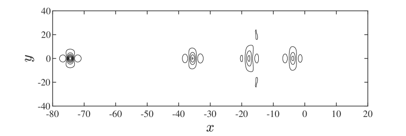
Next, we examine the transient solutions of the forced hydroelastic wave problem in the transcritical regime. Two representative cases of ice responses are shown in Fig. 11 and Fig. 12. For , a time-periodic shedding of lumps occurs, and these lumps propagate along three lines behind the forcing (see Fig. 11). We also check the cases of and , and the same phenomenon can be observed. It is found that if the forcing is moving at speed less than , lumps emerge merely along the negative -axis, and a typical example is shown in Fig. 12 for the forcing moving at . It seems plausible that the shedding routes of lumps vary with the forcing speed. For speeds closer to , say , more energy is accumulated, giving rise to multiple lumps released almost simultaneously. When the load speeds are a bit away from the phase speed minimum, less energy builds up, and only one lump forms at a time. Finally, Fig. 13 demonstrates the comparisons of - and -cross-sections between the resultant lump located at the leftmost edge of Fig. 12 and the exact solution, which show a remarkable agreement and validate our numerical codes as well.


4 Conclusion
In this paper, we are concerned with hydroelastic solitary waves on the surface of a three-dimensional fluid. The long-wave approximation is made, and a Benney-Luke-type equation possessing a Hamiltonian structure has been derived via the explicit non-local formulation of water waves introduced by Ablowitz et al. [23]. For the newly developed model, the associated BRDS system governing the envelope dynamics of a quasi-monochromatic plane wave has been established and numerically solved to help understand the existence, asymptotic behavior, and stability properties of solitary waves in the Benney-Luke-type equation.
For the unforced problem, three types of solitary waves, which can be predicted by a one-parameter family of solutions in the associated BRDS system, have been numerically computed in the Benney-Luke-type equation. We then discussed the asymptotic behavior of lumps based on the envelope equation, and it was shown that these lumps featured algebraically decaying tails in the far field. The transverse instability and subsequent evolution of plane solitary waves have been thoroughly explored. We proved that plane solitary waves were unstable subject to long-wavelength transverse perturbations and specified the critical perturbation wavenumber for the onset of instability, which coincided with the dimension-breaking bifurcation point. Numerical experiments have been conducted to verify these results, which showed that the transverse instability of plane solitary waves resulted in the emergence of depression lumps. Besides, interactions between lumps, including the head-on, overtaking, and oblique collisions, have also been investigated via numerical time integrations.
When a constant-moving load forces the problem, it has been found that there is a transcritical range of forcing speed where no permanent wave solutions can exist. Several numerical experiments have been carried out to study the transient responses to the forcing in the transcritical regime. The periodic shedding of lumps behind the forcing has been observed, indicating another generation mechanism of lumps. The shedding routes of lumps are qualitatively different for and , which should be relevant to the amount of accumulated energy during the period.
Finally, we should point out that our model can be extended by including the bottom topography and viscoelasticity of the plate. Therefore the Bernoulli equation can be rewritten as
The impermeability boundary condition at the bottom becomes
where the factor in the damping term is assumed to be constant, and is the bottom topography with . Following the same derivation procedure presented in §2, one can obtain
where the dimensionless damping coefficient is assumed to be .
Acknowledgement
This work was supported by the Key Research Program of Frontier Sciences of CAS (No. QYZDB-SSW-SYS015) and the Strategic Priority Research Program of CAS (No. XDB22040203).
References
- Squire et al. [1988] V. A. Squire, W. H. Robinson, P. J. Langhorne, and T. J. Haskell. Vehicles and aircraft on floating ice. Nature, 333:159–161, 1988.
- Takizawa [1985] T. Takizawa. Deflection of a floating sea ice sheet induced by a moving load. Cold Reg. Sci. Tech., 11(2):171–180, 1985.
- Van der Sanden and Short [2017] J. J. Van der Sanden and N. H. Short. Radar satellites measure ice cover displacements induced by moving vehicles. Cold Reg. Sci. Tech., 133:56–62, 2017.
- Părău and Dias [2002] E. I. Părău and F. Dias. Nonlinear effects in the response of a floating ice plate to a moving load. J. Fluid Mech., 460:281–305, 2002.
- Milewski et al. [2011] P. A. Milewski, J.-M. Vanden-Broeck, and Z. Wang. Hydroelastic solitary waves in deep water. J. Fluid Mech., 679:628–640, 2011.
- Milewski et al. [2013] P. A. Milewski, J.-M. Vanden-Broeck, and Z. Wang. Steady dark solitary flexural gravity waves. Proc. R. Soc. A, 469:20120485, 2013.
- Toland [2007] J. F. Toland. Heavy hydroelastic travelling waves. Proc. R. Soc. A, 463:2371–2397, 2007.
- Guyenne and Părău [2012] P. Guyenne and E. I. Părău. Computations of fully nonlinear hydroelastic solitary waves on deep water. J. Fluid Mech., 713:307–329, 2012.
- Wang et al. [2013] Z. Wang, J.-M. Vanden-Broeck, and P. A. Milewski. Two-dimensional flexural-gravity waves of finite amplitude in deep water. IMA J. Appl. Math., 78:750–761, 2013.
- Gao et al. [2016] T. Gao, Z. Wang, and J.-M. Vanden-Broeck. New hydroelastic solitary waves in deep water and their dynamics. J. Fluid Mech., 788:469–491, 2016.
- Gao and Vanden-Broeck [2014] T. Gao and J.-M. Vanden-Broeck. Numerical studies of two-dimensional hydroelastic periodic and generalised solitary waves. Phys. Fluids, 26(8):087101, 2014.
- Davys et al. [1985] J. W. Davys, R. J. Hosking, and A. D. Sneyd. Waves due to a steadily moving source on a floating ice plate. J. Fluid Mech., 158:269–287, 1985.
- Milinazzo et al. [1995] F. Milinazzo, M. Shinbrotand, and N. W. Evans. A mathematical analysis of the steady response of floating ice to the uniform motion of a rectangular load. J. Fluid Mech., 287:173–197, 1995.
- Părău and Vanden-Broeck [2011] E. I. Părău and J.-M. Vanden-Broeck. Three-dimensional waves beneath an ice sheet due to a steadily moving pressure. Phil. Trans. R. Soc. A, 369:2973–2988, 2011.
- Dinvay et al. [2019] E. Dinvay, H. Kalisch, and E. I. Părău. Fully dispersive models for moving loads on ice sheets. J. Fluid Mech., 876:122–149, 2019.
- Milewski and Wang [2013] P. A. Milewski and Z. Wang. Three dimensional flexural-gravity waves. Stud. Appl. Math., 131:135–148, 2013.
- Wang et al. [2014] Z. Wang, P. A. Milewski, and J.-M. Vanden-Broeck. Computation of three-dimensional flexural-gravity solitary waves in arbitrary depth. Procedia IUTAM, 11:119–129, 2014.
- Trichtchenko et al. [2018] O. Trichtchenko, E. I. Părău, J. M. Vanden-Broeck, and P. A. Milewski. Solitary flexural-gravity waves in three dimensions. Phil. Trans. R. Soc. A, 376(2129):20170345, 2018.
- Guyenne and Părău [2015] P. Guyenne and E. I. Părău. Asymptotic modeling and numerical simulation of solitary waves in a floating ice sheet equations of motion. In International Ocean and Polar Engineering Conference, 2015.
- Benney and Luke [1964] D. J. Benney and J. Luke. Interactions of permanent waves of finite amplitude. J. Math. Phys., 43(1-4):309–313, 1964.
- Pego and Quintero [1999] R. L. Pego and J. R. Quintero. Two-dimensional solitary waves for a Benney-luke equation. Physica D, 132:476–496, 1999.
- Berger and Milewski [2000] K. M. Berger and P. A. Milewski. The generation and evolution of lump solitary waves in surface-tension-dominated flows. SIAM J. Appl. Math., 61:731–750, 2000.
- Ablowitz et al. [2006] M. J. Ablowitz, A. S. Fokas, and Z. H. Musslimani. On a new non-local formulation of water waves. J. Fluid Mech., 562:313–343, 2006.
- Hărăgus-Courcelle and Andrej [1998] M. Hărăgus-Courcelle and I. Andrej. Three-dimensional solitary waves in the presence of additional surface effects. Eur. J. Mech. B-Fluid, 17(5):739–768, 1998.
- Xia and Shen [2002] X. Xia and H. T. Shen. Nonlinear interaction of ice cover with shallow water waves in channels. J. Fluid Mech., 467:259–268, 2002.
- Kim and Akylas [2005] B. Kim and T. R. Akylas. On gravity–capillary lumps. J. Fluid Mech., 540:337–351, 2005.
- Cipolatti [1992] R. Cipolatti. On the existence of standing waves for a davey-stewartson system. Commun. Part. Diff. Eq., 17(5-6):967–988, 1992.
- Alfimov et al. [1990] G. L. Alfimov, V. M. Eleonsky, N. E. Kulagin, L. M. Lerman, and V. P. Silin. On the existence of non-trivial solutions for the equation . Physica D, 44(1-2):168–177, 1990.
- Milewski and Wang [2014] P. A. Milewski and Z. Wang. Transversally periodic solitary gravity-capillary waves. Proc. R. Soc. A, 470:20130537, 2014.
- Wang and Milewski [2012] Z. Wang and P. A. Milewski. Dynamics of gravity-capillary solitary waves in deep water. J. Fluid Mech., 780:480–501, 2012.
- Petviashvili [1976] V. I. Petviashvili. Equation of an extraordinary soliton. Sov. J. Plasma Phys., 2:257–258, 1976.
- Kim and Akylas [2007] B. Kim and T. R. Akylas. Transverse instability of gravity-capillary solitary waves. J. Eng. Math., 58:167–175, 2007.
- Rypdal and Rasmussen [1989] K. Rypdal and J. J. Rasmussen. Stability of solitary structures in the nonlinear schrdinger equation. Physica Scripta, 40(2):192–201, 1989.
- Akers and Milewski [2009] B. Akers and P. A. Milewski. A model equation for wavepacket solitary waves arising from capillary-gravity flows. Stud. Appl. Math., 122:249–274, 2009.
- Wang and Vanden-Broeck [2015] Z. Wang and J.-M. Vanden-Broeck. Multi-lump symmetric and non-symmetric gravity-capillary solitary waves in deep water. SIAM J. Appl. Math., 75:978–998, 2015.
- Milewski and Tabak [1999] P. A. Milewski and E. G. Tabak. A pseudospectral procedure for the solution of nonlinear wave equations with examples from free-surface flows. SIAM J. Sci. Comput., 21:1102–1114, 1999.
- Wu [1987] T. Y. Wu. Generation of upstream advancing solitons by moving disturbances. J. Fluid Mech., 184:75–99, 1987.
- [38] J. Zhu. Internal solitons generated by moving disturbances. Ph.D. thesis, California Institute of Technology, Pasadena, CA.