Hybrid Quantum-Classical Eigensolver Without Variation or Parametric Gates
Abstract
The use of near-term quantum devices that lack quantum error correction, for addressing quantum chemistry and physics problems, requires hybrid quantum-classical algorithms and techniques. Here we present a process for obtaining the eigenenergy spectrum of electronic quantum systems. This is achieved by projecting the Hamiltonian of a quantum system onto a limited effective Hilbert space specified by a set of computational bases. From this projection an effective Hamiltonian is obtained. Furthermore, a process for preparing short depth quantum circuits to measure the corresponding diagonal and off-diagonal terms of the effective Hamiltonian is given, whereby quantum entanglement and ancilla qubits are used. The effective Hamiltonian is then diagonalized on a classical computer using numerical algorithms to obtain the eigenvalues. The use case of this approach is demonstrated for ground sate and excited states of BeH2 and LiH molecules, and the density of states, which agrees well with exact solutions. Additionally, hardware demonstration is presented using IBM quantum devices for H2 molecule.
I Introduction
Quantum computers offer the ability to address problems in quantum many-body chemistry and physics by quantum simulation or in a hybrid quantum-classical approach. The latter method is considered the most promising approach for noisy-intermediate scale quantum (NISQ) devices Preskill (2018). The prospect and benefits of quantum algorithms, along with suitable hardware, is in overcoming the complexity of the wave-function of a quantum system as it scales exponentially with system size McArdle et al. (2020). Therefore developing techniques and algorithms for NISQ era devices that may prove to have some computational advantage themselves, or establish a path towards ideas and foundations that provide advantage for future error-corrected quantum devices, is a worthwhile pursuit.
The leading algorithms intended to be executed on NISQ devices, which aim to determine solutions to an electronic Hamiltonian, are variational in nature Yuan et al. (2019). One specific algorithm is the variational quantum eigensolver (VQE), which has been tremendously successful in addressing chemistry and physics problems on quantum hardware and NISQ devices Peruzzo et al. (2014); McClean et al. (2016); Kandala et al. (2017); Barkoutsos et al. (2018); Jones et al. (2019); Nakanishi et al. (2019); Parrish et al. (2019a); Higgott et al. (2019); Jouzdani et al. (2019). However, the restriction or challenge that exist with VQE is the need for prior insight with regard to selecting the trial quantum state, i.e., ansatz circuit. Furthermore, the classical optimization of the ansatz parameters may be a poorly converging problem McClean et al. (2018); Parrish et al. (2019b) and therefore limiting the applicability of VQE for obtaining results accurate enough for chemical or physical interpretation. Finally, the realization of ansatz circuits that are motivated by domain knowledge, for example the unitary coupled cluster ansatz for chemistry problems Romero et al. (2017), may not be directly applicable on NISQ hardware and therefore requires clever modification to obtain hardware efficient ansätze Kandala et al. (2017); Barkoutsos et al. (2018); Herasymenko and O’Brien (2019).
In this work, we present a pragmatic hybrid quantum-classical approach for calculating the eigenenergy spectrum of a quantum system within an effective model. Firstly, an effective Hamiltonian is obtained through measurement of short-depth quantum circuits. The effective Hamiltonian is essentially the projection of the quantum system Hamiltonian onto a limited set of computational bases. The basis set is prepared with the intent of ensuring the dimensions of the corresponding matrix does not grow exponentially with the system size. In order to evaluate the matrix elements of the effective Hamiltonian, suitable non-parametric quantum circuits are specified. The quantum circuits are designed, executed, and measured. From the result of the measurements, the diagonal and off-diagonal terms of the effective Hamiltonian matrix are obtained. On the classical side, the effective Hamiltonian matrix, with suitable dimensions, is diagonalized numerically using a classical computer.
The paper is organized as follows: A short background is presented in Section II. In Section III the steps taken in our hybrid quantum-classical approach are explained in detail. In Section IV we demonstrate the application of this hybrid approach on simple chemical molecules BeH2 and LiH. In Section V the approach is demonstrated on the IBMQ 5-qubit Valencia quantum processor IBM-Q team (2020a) for H2 molecule. Finally, we discuss the integration of VQE and the proposed approach in Section VI.
II Background
Consider a quantum many-body system of electrons with the second quantized Hamiltonian:
| (1) |
and are the creation and annihilation operators, respectively. The anticommutator for the creation and annihilation are given by: and . These rules enforce the non-abelian group statistics for fermions, that is, under exchange of two fermions the wave-function yields a minus sign.
The indices in Eq. (1) refer to single-electron states. The coefficients and are the matrix integrals
| (2) |
and
| (3) |
where and operators correspond to one- and two-body interactions respectively. Since and can depend on other parameters, such as the distance between nuclei, the Hamiltonian in Eq. (1) represents a class of problems. However, this class of problems has the common property that the number of fermions is a conserved value. Strictly speaking, the terms in the Hamiltonian act on fixed-particle-number Hilbert spaces, , that have the correct fermionic antisymmetry, with denoting the number of electrons. In this paper, we consider this class of electronic systems where the Hamiltonian is assumed to be in the form of Eq. (1). The coefficients expressed in Eqs. (2–3) can be obtained using software packages developed for quantum chemistry calculations that perform efficient numerical integration Reine et al. (2012).
II.1 Mapping to qubits & computational basis
The Hamiltonian as written in Eq. (1) can be expressed in the form of qubit operations (i.e., Pauli matrices). This requires a transformation that preserves the anticommutation of the annihilation and creation operators. One transformation that satisfies the criteria, and is based on the physics of spin-lattice models, is the Jordan-Wigner (JW) transformation Fradkin (1989). The JW-transformed Hamiltonian takes the form
| (4) |
in which ’s are scalar and a Pauli string operator is defined as
| (5) |
acts on the -th qubit, are the three Pauli matrices Nielsen and Chuang (2002) and is the identity matrix with the number of qubits denoted as .
If the number of operators in the tensor product of is , we call a -local Pauli string operator. Upon the JW transformation of the Hamiltonian, a Fock basis of the second quantization representation is in one-to-one correspondence with a computational basis of the qubits Steudtner and Wehner (2019). In other words, a computational basis of
| (6) |
with qubits, where , is equivalent to a an antisymmetric Fock basis.
Within the finite, but exponentially large, Hilbert space spanned by computational basis set, an effective matrix representation of the Hamiltonian may be possible, specifically, if one can efficiently evaluate the matrix elements for an arbitrary computational basis and . Furthermore, assuming that the dimensions of the resulting effective matrix are relatively small, the matrix can be diagonalized on a classical computer, where its eigenvalues approximate the spectrum of the original Hamiltonian.
In this paper, we show how to evaluate a matrix element for arbitrary computational basis and , using a quantum circuit that has a circuit depth . We do so by using ancilla qubits, and thus physical resources are needed. In addition, we discuss how to choose an effective subspace for a given electronic Hamiltonian, with a dimension , based on physical motivations (see Section III.3). The condition makes it possible to diagonalize the Hamiltonian on a classical computer. In Section IV, we numerically demonstrate this method for simple quantum chemistry systems, focusing on ground state energy and the density of state calculations of the low-energy spectrum. Furthermore, in Section V we use the IBMQ 5-qubit Valencia device to measure the terms for H2 in the complete computational basis of 4 qubits.
III Constructing An Effective Matrix Representation for a Hamiltonian by Qubit Measurement
III.1 Effective Hamiltonian and circuit representation
We first consider a Hamiltonian that is expressed in terms of Pauli strings as in Eq. (4). Additionally, a subspace , with corresponding computational bases, is considered such that . Let us define the effective Hamiltonian matrix as the projection of onto this subspace; that is
| (7) |
The next step is to define a simple quantum circuit that utilizes one ancillary qubit to measure matrix element.
The dimension of depends on the choice of the subspace in . The choice of the subspace, intuitively, depends on the physics of the problem. However, the focus of this paper is towards quantum chemistry problems, which are a primary application for NISQ devices. For this class of Hamiltonians there is a systematic way to select the appropriate subspace. This is discussed in Section III.3.
The evaluation of diagonal terms in , e.g., , is trivially performed by preparing qubits as a bit string of and measuring . The measurement of the total Hamiltonian is obtained by measuring every individual Pauli string, , in Eq. (5). The diagonal terms are then given by
| (8) |
The off-diagonal matrix elements, e.g., , which are generally complex numbers, can be evaluated using a single ancillary qubit. This can be done by considering the quantum circuits as shown in Fig. 1. The two circuits shown in Fig. 1(a) and (b) are used to calculate the real and imaginary parts of the matrix element, respectively. In both circuits the qubits are initially prepared in state. The qubits are assumed to be enumerated linearly from to , where the -th qubit is the control qubit.


After applying the first Hadamard gate on the ancillary qubit, from left to right as shown in the circuits in Fig. 1(a–b), the quantum state of all the qubits is
| (9) |
which, after a sequence of controlled- gates, becomes entangled as
| (10) |
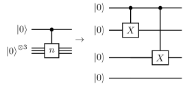
Here, control gates (controlled- and controlled-) flip qubits (corresponding to the occupied electronic states) and prepares the target qubits in the computational basis (), conditioned on the state of the control qubit is ().
An example of a controlled- gate that prepares target qubits in state is shown in Fig. 1(c). In practice, this part of the circuit requires two-qubit gates (e.g., CNOT) and perhaps the need for full connectivity of qubits in order to operate on any two qubits. Full connectivity of qubits could potentially be realized with ion-trapped devices Wright et al. (2019). See Section VI for further discussion.
Depending on whether the real part or the imaginary part is calculated, the last gates acting on the control qubit changes. With regard to the real part, after applying the last Hadamard gate on the control qubit in Fig. 1(a), the quantum state is
| (11) |
Using this prepared quantum state, one can measure
| (12) |
at the end of the circuit and have
Thus, after substituting for the diagonal elements and , using Eq. (8), one obtains the real part of the off-diagonal matrix element . The value in Eq. (LABEL:eq:subsec:idea:measurement-theory) is measured on a quantum device using the identity , by
| (14) | |||||
The imaginary part can be obtained in a similar fashion as done for the real part, but with a slight modification to the circuit as shown in Fig. 1(b). The key addition is a phase-gate, , before the execution of the last Hadamard gate on the control qubit. This yields the quantum state
| (15) |
that now includes a phase factor before . After the last Hadamard gate in Fig. 1(b), and following the same steps, Eqs. (12)-(14), the imaginary part is obtained.
Our approach differs from the typical hybrid quantum-classical paradigm used in ground state chemistry electronic structure calculations in that the quantum hardware is used as a coprocessor to measure these matrix elements. Therefore, no parameterized ansatz or variational optimization is required. In this approach, the depth of the quantum circuit is significantly reduced, however, our method is based on the assumption that the dimensions of in Eq. (7) are reasonable enough such that it can be diagonalized using classical numerical algorithms.
III.2 Implementing Measurements
As shown in Eq. (14), the expectation value of the Hamiltonian becomes the weighted sum of expectations for the set of Pauli string operators with respect to the output quantum state of the circuit. Since these operators are not in general commuting, one needs to setup and run a number of different quantum circuits. This number can be up-to all Pauli string operators in the Hamiltonian. Each circuit is then executed many times and every time the qubits are measured, the results are realized in different computational bases. The sampled realization provides a probability distribution and is used to estimate the expectation value of the Pauli string.
Generally, measurements are done either directly or indirectly. In the case of direct measurements, single-qubit rotations are applied to a subset of qubits at the end of the circuit. This subset is identified based on the locations in the tensor-product of the operator that are not identity . This set of rotations essentially changes the computational bases in which the given operator is diagonal. The direct measurement is commonly used in the experimental demonstration of quantum hardware and VQE Kandala et al. (2017).
The indirect measurement approach Knill et al. (2007) requires a series of controlled gates that are applied to the target qubits, using one ancillary control qubit. The indirect measurement method is used in iterative quantum phase estimation algorithms Dobšíček et al. (2007).
Although the two types of measurement approaches are theoretically equivalent Nielsen and Chuang (2002), experimentally, there are differences. The benefits and drawbacks of direct and indirect measurements are discussed for example in Mitarai and Fujii (2019). The main difference is the number of times the circuit is to be executed to achieve a desired precision , which is and for direct and indirect measurements respectively. The implementation of a general control- gate in the indirect measurement is a challenging task Knill et al. (2007). However, in regards to our purposed approach, where the operator is a single Pauli string, the indirect measurement implementation is straightforward.
The indirect measurement can be adapted as shown in quantum circuit in Fig. 2. An additional control qubit is added to this circuit. The Pauli operators are applied on the locations of when the control is in state . It is straightforward to follow the quantum state of the qubits throughout the circuit. The final state reads as:
| (16) |
Upon measuring , at the end of this circuit, using Eq. (16), and steps discussed in sec. III.1, the real part of the off-diagonal matrix element is obtained. The imaginary part is determined under same steps, while an additional phase gate is applied to the last ancillary qubit, similar to the situation in Fig. 1(b).
In terms of Pauli strings, the value of is obtained from the expectations , , and , similar to Eq. (14).

Finally, using the state preparation and measurements outlined through Sections III.1–III.2, all the matrix elements of the effective Hamiltonian in Eq. (7) can be evaluated, by repeating the execution of the quantum circuits as discussed in Figs. 1-2, for all the possible combinations of a chosen set of bases.
Note that the approach for evaluating the real and imaginary parts of a matrix element is similar to the interference method introduced in ref. Parrish et al. (2019a), with the difference being that our approach uses an ancillary qubit in order to realize the interference.
III.3 Preparing the computational basis
The computational basis set with , needs to be specified in practice. These bases serve as the row and columns of in Eq. (7). The process and motivation for how to choose this set should be based on the underlying nature and physics of the problem.
In theory, one established approach to approximate the ground states of quantum many-body systems is mean-field theory Jensen (2017). In this approach, the true ground state is constructed by perturbing a reference mean-field quantum state. The quantum chemistry field has established theories and techniques for treating such problems. One particularly successful theory and numerical method is coupled cluster (CC), typically referred to as the gold-standard in computational quantum chemistry Bartlett and Musiał (2007). In CC one assumes a wave-function ansatz
| (17) |
for the ground state. Here is a reference quantum state (e.g., Hartree-Fock) and is considered to be anti-symmetric under exchange of two fermions. The operator is a sum over different possible excitation operators with respect to the reference state. Typically, the set of excitation operators in includes single and double terms (i.e., CCSD), which enables a series representation of the Taylor expansion of , but high-order terms can also be added. The coefficients for the excitation operators inside are determined by variational methods; that is, by minimizing the expectation of the Hamiltonian with respect to the ansatz Bartlett and Musiał (2007).
Since the exponential operator in the CC ansatz, Eq. (17), is non-unitary, it cannot be directly implemented on gate-based quantum computers, where gates correspond to unitary operators. Thus, a unitary version of the CC ansatz has been introduced and is known as Unitary Coupled Cluster (UCC) Romero et al. (2017); Wecker et al. (2015). Ideally, the implementation of UCC ansatz should be constructed such that the number of gates is minimized so that the circuit depth does not exhaust the current coherence times of NISQ devices. As a result of the this concern, hardware efficient anstaz have been proposed Kandala et al. (2017) as a substitute.
In the numerical demonstration of this work (see Section IV), we consider a simplified ansatz for the ground state as:
| (18) | |||||
where refer to the unoccupied levels, and , refer to occupied levels with respect to single (S), double (D), and higher order excitation operators. The ansatz in Eq. (18) implies that the true many-body ground state is a superposition of the reference state and all possible S , D , up-to excitations, where in is finite and independent of .
In particular, assuming that it is possible to truncate the series at some low-excitation level such as the D or triples (T), the number of eigenstates in the expansion of the above ansatz remains a polynomial function in .
Taking the ansatz in Eq. (18), we specify the set in the following way. (1) Pick a computational basis as the reference quantum state, that is . (2) Identify computational bases corresponding to a finite number of excitations such as S and D. These are bases and polynomial function in .
In step (1), we identify the initial computational basis by minimizing the , in which, for example, a classical Monte Carlo process from spin lattice models Janke (1996) can be used. This computational basis is essentially the qubits’ configuration that has the lowest energy expectation. Since this step is a classical one, it is performed effectively even for a large number of qubits.
In step (2), once the state is determined, one can rearrange the configuration of the qubits by swapping ’s and ’s within the state . The swapping is done so that the configurations corresponding to S, D, up-to are fully realized. The energy expectation corresponding to these configurations (the diagonal elements in the ) are stored on a classical register. The final result is obtained among the set of configurations whereby of are the lowest energies; these are the configurations that are selected. The above steps are demonstrated numerically which is discussed in the next section (see Section IV).
IV Numerical Demonstration: LiH and BeH2
The application of the methodology discussed in Section III is focused on BeH2 and LiH molecules due to thier relatively small number of electrons and molecular orbital footprint. The number of electrons in BeH2 and LiH is six and four, respectively. The single-electron molecular spin-orbitals in the second quantized Hamiltonian are constructed using the minimal atomic STO-3G basis set Kandala et al. (2017); McArdle et al. (2020). For BeH2 there are a total of spin-orbital, and thus corresponds to qubits; LiH contains spin orbitals and hence qubits. For the purpose of measuring the matrix elements of the effective Hamiltonian, Eq. (7), one additional ancillary qubit is required, as illustrated in the quantum circuits shown in Fig. 1. Therefore, the total number of qubits for the simulation of BeH2 and LiH is and , respectively.
To obtain the coefficients in the Hamiltonian of Eq. (1) — more specifically as defined in Eqs. (2) and (3) — we make use of the Psi4 quantum chemistry package Parrish et al. (2017). The second quantized Hamiltonian is further transfomed onto a set of Pauli strings and their corresponding weights, Eq. (1), via JW transform using OpenFermion package McClean et al. (2017a).
In order to construct the potential energy surface for each inter-nuclear distance, , the steps indicated in the previous paragraph are repeated. The distance corresponds to the bond length between Be–H or Li–H in a given molecule; both LiH and BeH2 are linear molecules. We note that these calculations are assuming the total Hamiltonian can be represented using the Born-Oppenheimer approximation, where the dynamics of the core nuclei are neglected. This is standard practice in quantum chemistry calculations Jensen (2017) and thus at every distance , the nuclear-nuclear repulsion energy is treated classically and is added to the Hamiltonian as a constant.
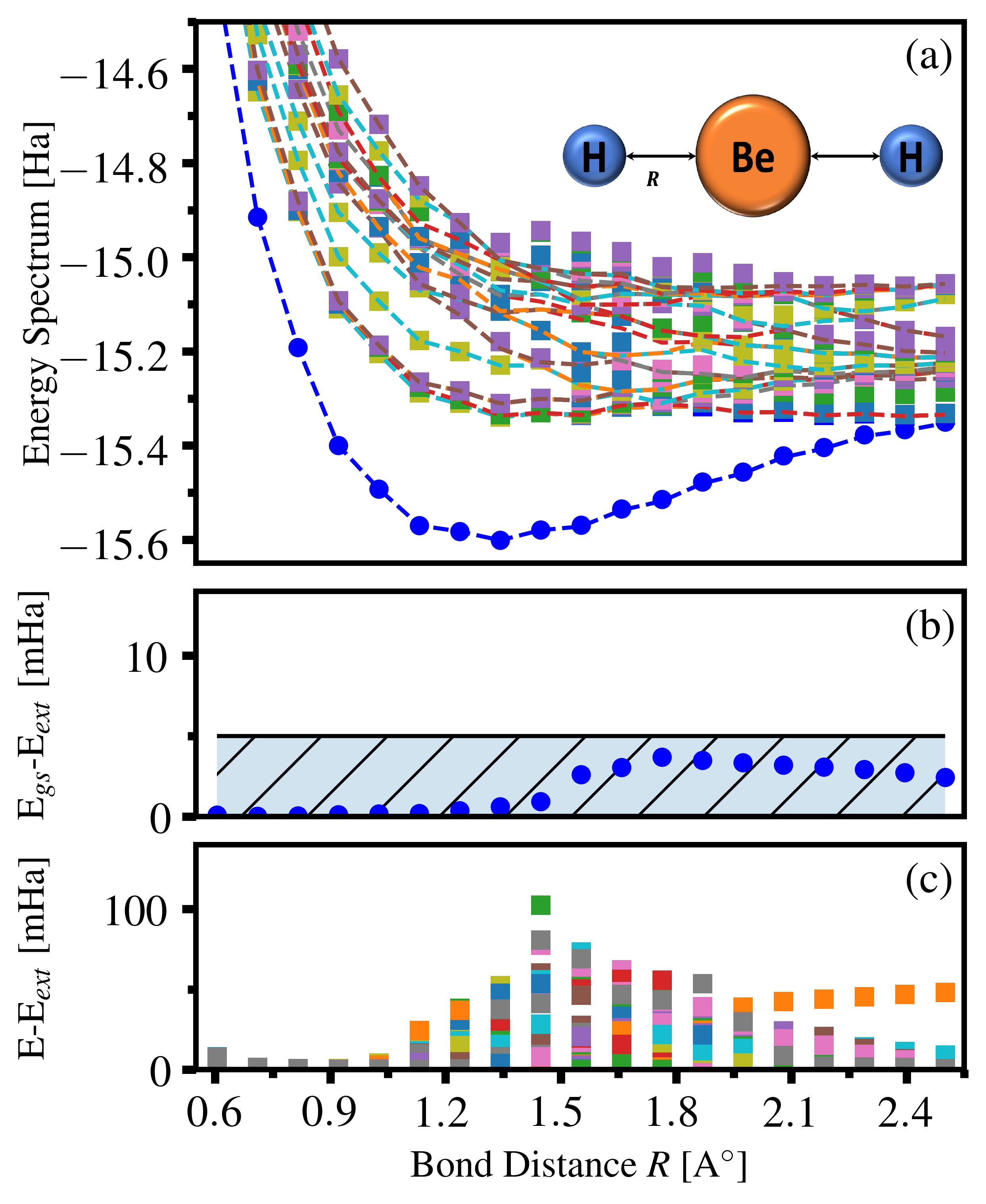
For every distance , a set of computational bases is chosen. This set includes the basis with the lowest energy expectation (the reference configuration) and computational bases that correspond to the low-order excitations (i.e., S, D, etc.) with respect to the reference configuration. In the case of BeH2, we construct the effective Hamiltonian matrix by keeping the S, D, and T excitations, and thus the total number of computational bases for BeH2 is . The low dimension of the effective Hamiltonian matrix makes it possible to diagonalize the matrix on a classical computer using standard numerical techniques Virtanen et al. (2020). Thus, the lowest energies, including the ground state energy, are obtained at every . The results for this process are shown in Fig. 3.
Fig. 3(a) shows the ground state energy as well as a few low-lying excited states for BeH2 of the effective Hamiltonian. The exact energies are given by the dashed curves in Fig. 3(a). In Fig. 3(b), the difference between the exact and obtained ground state energy is shown. An error within the hatched area indicates results that are within chemical accuracy. Chemical accuracy is typically identified as Hatrees. Figure 3(c) shows the same energy difference for all other excited-state energies. The same process is done for LiH where only S and D configurations are used. The total number of permutations of fermions () is reduced to , and the results are shown in Fig. 4.

The total number of configurations can be approximated by the highest excitation considered. For -electron excitation the number of configurations is . Thus, the total number of configurations is less than when . Of course, this argument is valid as long as can be assumed to be finite and independent of the size of the system or the number of electrons . Under these assumptions, the dimensions of the effective Hamiltonian, , remains polynomial if one replaces the minimal STO-3G with the extended atomic basis.
IV.1 Density of States
Knowledge of density of states (DOS) can be important in analyzing the thermodynamic behaviour of a system at finite temperature and in the analysis of transition states important in chemical reactions Truhlar et al. (1996). One advantage of the method proposed in this paper is the insights provided into the low-energy spectrum of the quantum system, more precisely, the degeneracy of the energy levels. To illustrate this, in Fig. 5, the unnormalized DOS of the LiH obtained via the effective Hamiltonian is compared with the exact density, which shows qualitatively good agreement.

V Hardware Demonstration: H2
In this section, we demonstrate the feasibility of the hybrid quantum-classical approach discussed in this paper on a IBMQ hardware device. Specifically, we calculate the eigenenergy spectrum of H2 molecule using STO-3G minimal basis-set.
Within STO-3G basis set, the total number of spin-orbitals for H2 is four. In contrast to the numerical demonstration, where the computational basis was prepared using the UCC ansatz, here we employ the complete computational basis with conserved number of electrons for H2 (). The number of computational basis set with conserved electron number, is , and the bases are:
| (19) | |||||
The number of bases is not further reduced; that is, the effective Hamiltonian constructed here is equal to the full Hamiltonian within the electron number. The above set can be interpreted as the collection of all the S and D exciations, as introduced in sub-section III.3, above a classical configuration such as .
The Hamiltonian of the problem, stated as a weighted sum of Pauli string operators, as in Eq. (4), has a total of fifteen operators, which can be grouped as:
| (20) | |||||
and
| (21) |
Here, a Pauli string operator such as is a shorthand for , as introduced in Eq. (5).
Our goal is to use the quantum hardware to evaluate the values for , where belongs to or , and and can be any of the bases listed in Eq. (19).
Note that this task is not a difficult one for a classical computer. However, the objective of the paper and hardware demonstration is to establish a hybrid quantum-classical computational scheme in which the quantum processor performs some of the computational tasks. In the simulations of this paper, the task is the evaluation of the phase associated with the exchange of fermions; since can be understood as exchanging fermions on via the operator , and to arrive at . The output can only take discrete values of , , and .
In each group and , Pauli string operators commute and thus, theoretically, can be measured simultaneously. However, in order to perform simultaneous measurement, one needs to adjust the computational bases, by applying further quantum gates on the target qubits. The appended measurement circuit further increases the circuit depth Gui et al. (2020). Thus, practically, the simultaneous measurement may not be advantageous, and, in contrast, induces further noise and decoherence on NISQ devices. Nevertheless, for , no further circuit depth is required, as they are all measured in the -basis.
We can further reduce the quantum coprocessor computational load by excluding circuits containing terms that are classically efficient to compute. In eqs. (20-21), the operators in do not contribute to off-diagonal matrix element of the Hamiltonian, while operators in contribute only to the off-diagonal matrix elements. This information is used to reduce the essential number of circuits to be run on the hardware.
The evaluation of an element is performed by assigning an appropriate circuit, as introduced in sub-section III.1, to a quantum coprocessor. In this work we make use of the IBMQ cloud open devices.
Once a circuit is loaded onto a quantum coprocessor, each circuit is executed a several times. The number of times a circuit is run is referred to as the number of shots. In this work, each circuit was executed for a total of shots. At each run, the qubits are measured, and the collection of the realized configurations is used to evaluate value of .
The preparation of the circuits is performed using the transpile and assemble routines available in the IBM Qiskit API Abraham et al. (2019), which enables collating individual circuits, corresponding to the diagonal and off-diagonal terms, to prepare each circuit to run as a single job on a target IBMQ device. In this work, we make use of the IBMQ 5-qubit Valencia hardware IBM-Q team (2020a). The number of circuits — for both real and imaginary parts separately — after the transpile and assemble routines for the diagonal and off-diagonal terms corresponds to 66 and 60 circuits, respectively. The execution timings for the IBMQ QASM simulator range between 0.21-1.5 seconds and for the IBMQ Valencia 5 qubit device 274-298 seconds with 8000 shots per circuit. Due to the limited number of qubits available on this processor, direct measurement is used, that is by measuring all the qubits at the end of the circuit.
As a sanity check, we first use IBMQ QASM simulator IBM-Q team (2020b) to perform all steps involved as outlined in III. The calculations are shown in Fig. 6(a). The results perfectly match the exact values as expected. Furthermore, in Fig. 6(b) the off-diagonal terms in the Hamiltonian are evaluated using IBMQ Valencia device, while the diagonal elements are evaluated using the IBMQ QASM simulator. In both cases, upon diagonalization of the obtained Hamiltonian, the energy spectrum is in good agreement with the exact values. We observe in Fig. 6(b) that there is a slight lifting of the double degeneracy of H2, which we associate to the device noise. This is due to the occurance of non-zero values in the measured off-diagonal terms when in fact the exact value should be zero.
Finally, all the matrix elements, that is, diagonal and off-diagonal elements, are evaluated using IBMQ Valencia device. The results are shown in Fig. 7-(a), which was done with and without measurement error mitigation. The use of measurement error mitigation marginally improves the results. The discrepancy between the exact and hardware values, without and with measurement error mitigation, are shown in 7(b-c).
The effect of noise is ubiquitous in current quantum hardware and is inherently complex and difficult to characterize. However, the result of noise due to the measurement process can be mitigated to some degree by using a calibration matrix Abraham et al. (2019). The resulting calibration matrix is then used to reduce errors of subsequent circuit measurements. The application of measurement error mitigation is demonstrated in Fig. 7(a) with beneficial impact on error shown in Fig. 7(c).
The calculations in Fig. 7, that is construction of the effective Hamiltonian, , are performed through five independent IBMQ job submissions. Each time the energy-surface is slightly different, which can be associated to the inherent device errors and perhaps low number of shots used. The error bars in Fig. 7(b-c) indicate the min/max range in errors of the five different calculation.


VI Discussion and Summary
Recently an abundance of Variational Quantum Algorithms (VQA) have been introduced to solve electronic quantum many-body problems on NISQ devices Peruzzo et al. (2014); Wecker et al. (2015); McClean et al. (2016); Yuan et al. (2019); Parrish et al. (2019a); Higgott et al. (2019); Jones et al. (2019); Nakanishi et al. (2019). These VQA proposals mostly rely on optimization of parametric circuits. In this paper we demonstrate that an alternative approach exists, specifically for quantum chemistry problems, which does not require an optimization procedure and parametric ansatz. In this approach, the quantum hardware is used only to prepare a many-body quantum state and to efficiently measure the expectation values of certain target observables with respect to this quantum state. From the output measurements, one can construct what we refer to as an effective Hamiltonian matrix, . Upon diagonalization of using classical eigen-decomposition numerical methods one obtains the ground state and low-lying excited states of the system.
The approach introduced in this paper is particularly suitable for NISQ devices where short quantum circuit depth is essential due to lack of error-correction protocols on these devices. An additional important aspect of this approach is that it provides access to the low-lying energy spectra of the system and not just the ground state in comparison with the original VQE process.
In the context of VQE and VQE-type algorithms, several attempts have been made to extend the variational approach to excited states Tilly et al. (2020); Santagati et al. (2018); Higgott et al. (2019); McArdle et al. (2019); Somma (2019); Parrish et al. (2019a). Quantum subspace expansion McClean et al. (2017b); Colless et al. (2018) for example constructs a set of non-orthogonal bases out of an optimized ansatz, and performs post-processing to obtain excited states. Deflation techniques as described in ref. Higgott et al. (2019), constructs a pseudo-Hamiltonian in which the ground state is excluded and orthogonality is enforced through regularization. Successful examples are introduced for some low-lying excited states of LiH Jones et al. (2019). In all these previous works, optimization of a parametric ansatz is required therefore necessitates an enormous number of quantum circuit executions and sampling.
The approach introduced in this paper is similar to multistate contracted VQE (MC-VQE) in ref. Parrish et al. (2019a). The main difference is the application of VQE: MC-VQE is obviously a VQE-type algorithm, our approach is distinct in that it does not require a parametric circuit or variational procedure for optimization. In addition, our method differs since it uses supporting quantum circuit resources, i.e., ancilla qubits, in order to perform interference and measurement that is different from the quantum circuit in ref. Diker (2016) and its generalization in ref. Parrish et al. (2019a).
An extension of our approach to VQE type algorithm is possible. This can be done by appending a set of parametric gates that act only on the target qubits to the circuits in Fig. 1. Let us denote this part of the circuit with , where stands for a set of parameters. Then, it can be verified that, given , the final matrix element obtained from the circuit after measurement (see Eq. (2) for example) becomes , compared to . The appended parametric circuit allows one to project the Hamiltonian onto , for a given . This means the effective Hamiltonian is now parametric and depends on the value(s) of . The optimal parameter(s) are then obtained by minimizing the ground-state energy of the effective Hamiltonian matrix. The reference state can be regarded as the contracted reference states introduced in ref. Parrish et al. (2019a).
One possible limitation of the circuits shown in Fig. 1 is the execution of two-qubit gates corresponding to control operations over -qubits (i.e., series of CNOT gates). For NISQ devices with hardware-restricted qubit connectivity, this may require a number of SWAP gate operations and therefore can increase the circuit depth and subsequent error rates Venturelli et al. (2018); Nash et al. (2020). In essence, the implementation of the circuits described in this paper will depend on the ability to limit circuit depth and associated error rates by NISQ hardware circuit optimization (i.e., scheduling). However, significant improvements in qubit connectivity of various modalities (e.g., ion traps) Wright et al. (2019); Hazra et al. (2020) or optimizing quantum circuits against decoherence Zhang et al. (2019); Holmes et al. (2020) may blunt this concern.
VII Acknowledgement
The ideas and methodology discussed in Section III have been supported by General Atomics internal R&D funds. Their application towards quantum chemistry problems as discussed in Section IV and Section V is based upon work supported by the U.S. Department of Energy, Office of Science, Office of Fusion Energy Sciences, under Award Number DE-SC0020249. We thank Mark Kostuk for his guidance and management as PI under this grant. Additionally, we thank David P. Schissel for feedback and guidance at General Atomics.
Circuit diagrams are rendered using the LaTeX Quantikz package Kay (2019), numerical scripts utilize the Python SciPy package Virtanen et al. (2020), and 2D plots are generated with the Python matplotlib package Hunter (2007). We acknowledge use of the IBMQ for this work. The views expressed are those of the authors and do not reflect the official policy or position of IBM or the IBMQ team.
Disclaimer: A portion of this report was prepared as an account of work sponsored by an agency of the United States Government. Neither the United States Government nor any agency thereof, nor any of their employees, makes any warranty, express or implied, or assumes any legal liability or responsibility for the accuracy, completeness, or usefulness of any information, apparatus, product, or process disclosed, or represents that its use would not infringe privately owned rights. Reference herein to any specific commercial product, process, or service by trade name, trademark, manufacturer, or otherwise does not necessarily constitute or imply its endorsement, recommendation, or favoring by the United States Government or any agency thereof. The views and opinions of authors expressed herein do not necessarily state or reflect those of the United States Government or any agency thereof.
References
- Preskill (2018) J. Preskill, Quantum 2, 79 (2018), ISSN 2521-327X, URL https://doi.org/10.22331/q-2018-08-06-79.
- McArdle et al. (2020) S. McArdle, S. Endo, A. Aspuru-Guzik, S. C. Benjamin, and X. Yuan, Reviews of Modern Physics 92, 015003 (2020).
- Yuan et al. (2019) X. Yuan, S. Endo, Q. Zhao, Y. Li, and S. C. Benjamin, Quantum 3, 191 (2019).
- Peruzzo et al. (2014) A. Peruzzo, J. McClean, P. Shadbolt, M.-H. Yung, X.-Q. Zhou, P. J. Love, A. Aspuru-Guzik, and J. L. O’brien, Nature communications 5, 4213 (2014).
- McClean et al. (2016) J. R. McClean, J. Romero, R. Babbush, and A. Aspuru-Guzik, New Journal of Physics 18 (2016), ISSN 13672630, eprint 1509.04279.
- Kandala et al. (2017) A. Kandala, A. Mezzacapo, K. Temme, M. Takita, M. Brink, J. M. Chow, and J. M. Gambetta, Nature 549, 242 (2017).
- Barkoutsos et al. (2018) P. K. Barkoutsos, J. F. Gonthier, I. Sokolov, N. Moll, G. Salis, A. Fuhrer, M. Ganzhorn, D. J. Egger, M. Troyer, A. Mezzacapo, et al., Phys. Rev. A 98, 022322 (2018), URL https://link.aps.org/doi/10.1103/PhysRevA.98.022322.
- Jones et al. (2019) T. Jones, S. Endo, S. McArdle, X. Yuan, and S. C. Benjamin, Phys. Rev. A 99, 062304 (2019), URL https://link.aps.org/doi/10.1103/PhysRevA.99.062304.
- Nakanishi et al. (2019) K. M. Nakanishi, K. Mitarai, and K. Fujii, Phys. Rev. Research 1, 033062 (2019), URL https://link.aps.org/doi/10.1103/PhysRevResearch.1.033062.
- Parrish et al. (2019a) R. M. Parrish, E. G. Hohenstein, P. L. McMahon, and T. J. Martínez, Phys. Rev. Lett. 122, 230401 (2019a), URL https://link.aps.org/doi/10.1103/PhysRevLett.122.230401.
- Higgott et al. (2019) O. Higgott, D. Wang, and S. Brierley, Quantum 3, 156 (2019), ISSN 2521-327X, URL https://doi.org/10.22331/q-2019-07-01-156.
- Jouzdani et al. (2019) P. Jouzdani, S. Bringuier, and M. Kostuk, A method of determining excited-states for quantum computation (2019), eprint arXiv:1908.05238.
- McClean et al. (2018) J. R. McClean, S. Boixo, V. N. Smelyanskiy, R. Babbush, and H. Neven, Nature communications 9, 1 (2018).
- Parrish et al. (2019b) R. M. Parrish, J. T. Iosue, A. Ozaeta, and P. L. McMahon, A jacobi diagonalization and anderson acceleration algorithm for variational quantum algorithm parameter optimization (2019b), eprint arXiv:1904.03206.
- Romero et al. (2017) J. Romero, R. Babbush, J. R. McClean, C. Hempel, P. Love, and A. Aspuru-Guzik, Strategies for quantum computing molecular energies using the unitary coupled cluster ansatz (2017), eprint arXiv:1701.02691.
- Herasymenko and O’Brien (2019) Y. Herasymenko and T. E. O’Brien, A diagrammatic approach to variational quantum ansatz construction (2019), eprint 1907.08157.
- IBM-Q team (2020a) IBM-Q team, IBM-Q 5 Qubit Valencia backend, specification v1.3.1 (2020a), retrieved from https://quantum-computing.ibm.com.
- Reine et al. (2012) S. Reine, T. Helgaker, and R. Lindh, Wiley Interdisciplinary Reviews: Computational Molecular Science 2, 290 (2012).
- Fradkin (1989) E. Fradkin, Physical review letters 63, 322 (1989).
- Nielsen and Chuang (2002) M. A. Nielsen and I. Chuang, Quantum computation and quantum information (American Association of Physics Teachers, 2002).
- Steudtner and Wehner (2019) M. Steudtner and S. Wehner, Phys. Rev. A 99, 022308 (2019), URL https://link.aps.org/doi/10.1103/PhysRevA.99.022308.
- Wright et al. (2019) K. Wright, K. M. Beck, S. Debnath, J. M. Amini, Y. Nam, N. Grzesiak, J.-S. Chen, N. C. Pisenti, M. Chmielewski, C. Collins, et al., Nature Communications 10 (2019), ISSN 2041-1723, URL http://dx.doi.org/10.1038/s41467-019-13534-2.
- Knill et al. (2007) E. Knill, G. Ortiz, and R. D. Somma, Phys. Rev. A 75, 012328 (2007), URL https://link.aps.org/doi/10.1103/PhysRevA.75.012328.
- Dobšíček et al. (2007) M. Dobšíček, G. Johansson, V. Shumeiko, and G. Wendin, Phys. Rev. A 76, 030306 (2007), URL https://link.aps.org/doi/10.1103/PhysRevA.76.030306.
- Mitarai and Fujii (2019) K. Mitarai and K. Fujii, Phys. Rev. Research 1, 013006 (2019), URL https://link.aps.org/doi/10.1103/PhysRevResearch.1.013006.
- Jensen (2017) F. Jensen, Introduction to computational chemistry (John wiley & sons, 2017).
- Bartlett and Musiał (2007) R. J. Bartlett and M. Musiał, Reviews of Modern Physics 79, 291 (2007).
- Wecker et al. (2015) D. Wecker, M. B. Hastings, and M. Troyer, Phys. Rev. A 92, 042303 (2015), URL https://link.aps.org/doi/10.1103/PhysRevA.92.042303.
- Janke (1996) W. Janke, Monte Carlo Simulations of Spin Systems (Springer Berlin Heidelberg, Berlin, Heidelberg, 1996), pp. 10–43, ISBN 978-3-642-85238-1, URL https://doi.org/10.1007/978-3-642-85238-1_3.
- Parrish et al. (2017) R. M. Parrish, L. A. Burns, D. G. A. Smith, A. C. Simmonett, A. E. DePrince, E. G. Hohenstein, U. Bozkaya, A. Y. Sokolov, R. Di Remigio, R. M. Richard, et al., Journal of Chemical Theory and Computation 13, 3185 (2017), URL https://doi.org/10.1021/acs.jctc.7b00174.
- McClean et al. (2017a) J. R. McClean, K. J. Sung, I. D. Kivlichan, Y. Cao, C. Dai, E. S. Fried, C. Gidney, B. Gimby, P. Gokhale, T. Häner, et al., Openfermion: The electronic structure package for quantum computers (2017a), eprint 1710.07629.
- Virtanen et al. (2020) P. Virtanen, R. Gommers, T. E. Oliphant, M. Haberland, T. Reddy, D. Cournapeau, E. Burovski, P. Peterson, W. Weckesser, J. Bright, et al., Nature Methods (2020).
- Truhlar et al. (1996) D. G. Truhlar, B. C. Garrett, and S. J. Klippenstein, The Journal of physical chemistry 100, 12771 (1996).
- Gui et al. (2020) K. Gui, T. Tomesh, P. Gokhale, Y. Shi, F. T. Chong, M. Martonosi, and M. Suchara, Term grouping and travelling salesperson for digital quantum simulation (2020), eprint 2001.05983.
- Abraham et al. (2019) H. Abraham, AduOffei, R. Agarwal, I. Y. Akhalwaya, G. Aleksandrowicz, T. Alexander, M. Amy, E. Arbel, A. Asfaw, A. Avkhadiev, et al., Qiskit: An open-source framework for quantum computing (2019).
- IBM-Q team (2020b) IBM-Q team, IBM-Q QASM backend, specification v0.1.547 (2020b), retrieved from https://quantum-computing.ibm.com.
- Tilly et al. (2020) J. Tilly, G. Jones, H. Chen, L. Wossnig, and E. Grant (2020), eprint arXiv:2001.04941.
- Santagati et al. (2018) R. Santagati, J. Wang, A. A. Gentile, S. Paesani, N. Wiebe, J. R. McClean, S. Morley-Short, P. J. Shadbolt, D. Bonneau, J. W. Silverstone, et al., Science Advances 4 (2018), eprint arXiv:1611.03511.
- McArdle et al. (2019) S. McArdle, T. Jones, S. Endo, Y. Li, S. C. Benjamin, and X. Yuan, npj Quantum Information 5 (2019), ISSN 2056-6387, URL http://dx.doi.org/10.1038/s41534-019-0187-2.
- Somma (2019) R. D. Somma, Quantum eigenvalue estimation via time series analysis (2019), eprint 1907.11748.
- McClean et al. (2017b) J. R. McClean, M. E. Kimchi-Schwartz, J. Carter, and W. A. de Jong, Physical Review A 95 (2017b), ISSN 2469-9934, URL http://dx.doi.org/10.1103/PhysRevA.95.042308.
- Colless et al. (2018) J. I. Colless, V. V. Ramasesh, D. Dahlen, M. S. Blok, M. E. Kimchi-Schwartz, J. R. McClean, J. Carter, W. A. de Jong, and I. Siddiqi, Phys. Rev. X 8, 011021 (2018), URL https://link.aps.org/doi/10.1103/PhysRevX.8.011021.
- Diker (2016) F. Diker, Deterministic construction of arbitrary states with quadratically increasing number of two-qubit gates (2016), eprint arXiv:1606.09290.
- Venturelli et al. (2018) D. Venturelli, M. Do, E. Rieffel, and J. Frank, Quantum Science and Technology 3, 025004 (2018), URL https://doi.org/10.1088%2F2058-9565%2Faaa331.
- Nash et al. (2020) B. Nash, V. Gheorghiu, and M. Mosca, Quantum Science and Technology 5, 025010 (2020), URL https://doi.org/10.1088%2F2058-9565%2Fab79b1.
- Hazra et al. (2020) S. Hazra, K. V. Salunkhe, A. Bhattacharjee, G. Bothara, S. Kundu, T. Roy, M. P. Patankar, and R. Vijay, Applied Physics Letters 116, 152601 (2020), eprint https://doi.org/10.1063/1.5143440, URL https://doi.org/10.1063/1.5143440.
- Zhang et al. (2019) Y. Zhang, H. Deng, Q. Li, H. Song, and L. Nie, in 2019 International Symposium on Theoretical Aspects of Software Engineering (TASE) (IEEE, 2019), pp. 184–191.
- Holmes et al. (2020) A. Holmes, M. R. Jokar, G. Pasandi, Y. Ding, M. Pedram, and F. T. Chong, arXiv preprint arXiv:2004.04794 (2020), eprint 2004.04794.
- Kay (2019) A. Kay (2019), URL https://royalholloway.figshare.com/articles/Quantikz/7000520.
- Hunter (2007) J. D. Hunter, Computing in Science & Engineering 9, 90 (2007).