Hybrid Feedback for Global Tracking on Matrix Lie Groups and
Abstract
We introduce a new hybrid control strategy, which is conceptually different from the commonly used synergistic hybrid approaches, to efficiently deal with the problem of the undesired equilibria that precludes smooth vectors fields on from achieving global stability. The key idea consists in constructing a suitable potential function on involving an auxiliary scalar variable, with flow and jump dynamics, which keeps the state away from the undesired critical points while, at the same time, guarantees a decrease of the potential function over the flows and jumps. Based on this new hybrid mechanism, a hybrid feedback control scheme for the attitude tracking problem on , endowed with global asymptotic stability and semi-global exponential stability guarantees, is proposed. This control scheme is further improved through a smoothing mechanism that removes the discontinuities in the input torque. The third hybrid control scheme, proposed in this paper, removes the requirement of the angular velocity measurements, while preserving the strong stability guarantees of the first hybrid control scheme. This approach has also been applied to the tracking problem on to illustrate its advantages with respect to the existing synergistic hybrid approaches. Finally, some simulation results are presented to illustrate the performance of the proposed hybrid controllers.
Index Terms:
Attitude control, Hybrid feedback, Rigid body system, Velocity-free feedback, Matrix Lie group,I Introduction
The attitude tracking control problem of rigid body systems has been widely investigated in the literature with many applications related to robotics, aerospace and marine engineering, for instance [2, 3, 4, 5, 6, 7]. In particular, geometric control design on Lie groups and , has generated a great deal of research work [8, 9, 10, 11, 6, 12, 13]. It is well known that achieving global stability results with feedback control schemes designed on Lie groups such as and , is a fundamentally difficult task due to the topological obstruction of the motion space induced by the fact that these manifolds are not homeomorphic to and that there is no smooth vector field that can have a global attractor [8]. To achieve almost global asymptotic stability (AGAS), a class of suitable “navigation functions” has been introduced in [8]. In [9], the Riemannian structure of the configuration manifold for a class of mechanical systems, is used to derive a local exponential control law, while in [11], an almost global tracking controller has been proposed for a general class of Lie groups via intrinsic globally-defined error dynamics. It is well known that for any smooth potential function on , there exist at least four critical points where its gradient vanishes [14], and as such, almost global stability is the strongest result that one can achieve in this case.
Using the hybrid dynamical systems framework of [15, 16], a unit-quaternion based hybrid control scheme for global attitude tracking was first proposed in [17], which led thereafter to other variants such as [18, 19, 20]. The use of a “synergistic” family of potential functions to overcome the topological obstruction to global asymptotic stability (GAS) on has been introduced in [21]. A family of potential functions is “centrally” synergistic, if the identity is the common critical point of all the potential functions in the family. This synergistic hybrid approach was successfully applied to the rigid body attitude control problem in [22], where a hysteresis-based switching mechanism was introduced to avoid all the undesired critical points and ensure some robustness to measurement noise. However, only numerical examples were provided to construct such a synergistic family of potential functions via angular warping on . Inspired by this, a number of hybrid controllers and observers on Lie groups , and have been proposed in the literature [23, 24, 25, 26, 27, 28, 29, 30, 31]. The work in [26], provides a systematic and comprehensive procedure for the construction of synergistic potential functions on , which is then applied to design velocity-free hybrid attitude stabilization and tracking control schemes [26, 27]. Moreover, a hybrid attitude control scheme on using an “exp-synergistic” family of potential functions, leading to global exponential stability, has been proposed in [28]. Alternatively, a “non-central” synergistic family of potential functions has been considered in [23] to relax the centrality condition. A similar idea can be found in [25]. Recently, a hybrid control approach on smooth manifolds, relying on a switching logic between local coordinates, has been proposed in [32].
Contributions: In this paper, we propose new hybrid feedback control strategies for the tracking problems on matrix Lie groups and , leading to GAS guarantees. Some extensions are also proposed to smooth out the discontinuities induced by the control input switching, and to handle the lack of angular velocity measurements. The main novelty and strength of our approach is the fact that it can overcome the compactness condition required in the synergistic hybrid approaches. Therefore, it can be applied to a general class of non-compact matrix Lie groups to generate globally asymptotically stabilizing hybrid feedback laws as demonstrated through the design of a geometric hybrid tracking control scheme on the non-compact manifold . The key idea of our hybrid attitude control strategy consists in using a suitable potential function on involving an auxiliary scalar variable with hybrid dynamics. This scalar variable is governed by some appropriately designed flow dynamics when the state in is away from the undesired critical points, and is governed by an appropriately designed jump strategy when the state is in the neighborhood of the undesired critical points. The flow and jump strategies are designed to ensure a decrease of the potential function over the flows and jumps. In contrast with the synergistic hybrid approaches where a synergistic family of potential functions on is used [22, 21, 23, 26, 27], our hybrid approach relies on a single potential function on parameterized by the hybrid auxiliary scalar variable. As it is going to be shown later, our approach on top of the hybrid control design simplification, allows to overcome the set compactness assumption (stemming from the diffeomorphism condition of the transformation map) required in the synergistic hybrid approaches. This important advantage, makes our approach a good candidate for the design of hybrid controllers on non-compact manifold such as where the existing hybrid approaches (for instance, [22, 21, 25, 26, 28, 27, 32]) are not applicable in a straightforward manner. A preliminary version of this work has been presented in [1] without the semi-global exponential stability proof, the control smoothing mechanism and the velocity-free hybrid tracking scheme presented in the present paper.
Organization: The remainder of this paper is organized as follows: Section II provides the preliminaries that will be used throughout this paper. In Section III, we formulate our attitude tracking control problem. In Section IV, a new hybrid mechanism using a potential function on is presented. In Sections V-VII, we present our three hybrid attitude tracking controllers. In Section VIII, we provide a systematic procedure for the construction of the potential function on satisfying all the requirements for the design of our hybrid attitude tracking controllers. In Section IX, our hybrid control strategy is extended to the pose tracking problem on the non-compact Lie group . Simulation results are presented in Section X.
II Preliminaries
II-A Notations and Definitions
The sets of real, non-negative real and natural numbers are denoted by , and , respectively. We denote by the -dimensional Euclidean space, and by the set of unit vectors in . Given two matrices, , their Euclidean inner product is defined as . The Euclidean norm of a vector is denoted by , and the Frobenius norm a matrix is denoted by . For a given symmetric matrix , we define as the set of all the unit-eigenvectors of , as the -th pair of eigenvalue and eigenvector of , and and as the minimum and maximum eigenvalue of , respectively. Let be a smooth manifold embedded in and be the tangent space on at point . The gradient of a differentiable real-valued function at point , denoted by , relative to the Riemannian metric is uniquely defined by for all . A point is called a critical point of if its gradient at varnishes (i.e., ). A continuously differentiable function is said to be a potential function on with respect to the set if for all and for all .
The 3-dimensional Special Orthogonal group is defined by , and the Lie algebra of is defined by . The tangent space of at any base point is defined by . The inner product in the tangent space defines the left invariant metric on as for all and . For any , we define as the normalized Euclidean distance on with respect to the identity , which is given by . Let the map represent the well-known angle-axis parameterization of the attitude, which is given by with denoting the rotation angle and denoting the rotation axis. For a given vector , we define as the skew-symmetric matrix given by
and as the inverse operator of the map , such that . For a matrix , we denote as the anti-symmetric projection of . Define the composition map such that, for a matrix , one has For any , one can verify that
II-B Hybrid Systems Framework
Consider a smooth manifold embedded in and its tangent bundle denoted by . A general model of a hybrid system is given as [15]:
| (1) |
where denotes the state, denotes the state after an instantaneous jump, the flow map describes the continuous flow of on the flow set , and the jump map (a set-valued mapping from to ) describes the discrete jumps of on the jump set . A solution to is parameterized by , where denotes the amount of time passed and denotes the number of discrete jumps that have occurred. A subset is a hybrid time domain if for every , the set, denoted by , is a union of finite intervals of the form with a time sequence . A solution to is said to be maximal if it cannot be extended by flowing nor jumping, and complete if its domain is unbounded. Let denote the distance of a point to a closed set , and then the set is said to be: stable for if for each there exists such that each maximal solution to with satisfies for all ; globally attractive for if every maximal solution to is complete and satisfies for all ; globally asymptotically stable if it is both stable and globally attractive for . Moreover, the is said to be (locally) exponentially stable for if there exist such that, for any , every maximal solution to is complete and satisfies for all [33]. We refer the reader to [15, 16] and references therein for more details on hybrid dynamical systems.
III Problem Formulation
The dynamical equations of motion of a rigid body on are given by
| (2) |
where the rotation matrix denotes the attitude of the rigid body, is the body-frame angular velocity, is the inertia matrix (constant and known), and is the control torque to be designed.
Let and let be a compact (closed and bounded) subset. Let the desired reference trajectory be generated by the following dynamical system [23]:
| (6) |
where and are the desired rotation and angular velocity, and is the closed ball in . As shown in [23], every maximal solution to (6) is complete, and any possible solution component of (6) is Lipschitz continuous with Lipschitz constant , but not necessarily differentiable.
Let us consider the left-invariant attitude tracking error and the angular velocity tracking error . From (2)-(6), one obtains the following error dynamics [23]:
| (7a) | ||||
| (7b) | ||||
where the functions and are given by
| (8a) | ||||
| (8b) | ||||
Note that is skew-symmetric, and as such, for each one has . It is clear that is known, and if is constant.
IV A new Hybrid Mechanism Using a Single Potential Function on
Let be a potential function on with respect to . Let denote the gradient of at point . According to Lusternik-Schnirelmann theorem [34] and Morse theory [14], a smooth vector field on can not have a global attractor, and any smooth potential function on must have at least four critical points. Let the set of all critical points of be denoted by , and the set of all undesired critical points be denoted by .
One possible way to make the desired critical point a global attractor, consists in generating a non-smooth gradient-based vector field on through a switching mechanism between a family of potential functions as done in [22, 21, 26]. The potential functions are constructed using a modified trace function and a transformation map such that all the potential functions share only the desired critical point . For instance, a transformation map with , known as the “angular warping”, is considered in [21]. As shown in [21, Theorem 8], is required to be a diffeomorphism, and to be as such, has to be chosen sufficiently small in magnitude (i.e., for all ). A similar design of the central synergistic family of potential functions can be found in [26], where a different transformation map with and sufficiently small, has been considered. Note that the existence of the parameter in [22, 21, 26] is guaranteed mainly due to the fact that is compact. Alternatively, in [23], a non-central synergistic family of potential functions has been designed based on a modified trace function through constant translation, scaling and biasing. Unfortunately, it is not straightforward to explicitly construct such a family of potential functions, especially when dealing with systems evolving on non-compact manifolds.
To overcome the above mentioned problems, we propose a new approach that does not require the generation of a family of potential functions via a diffeomorphism map, leading to a much simpler design of hybrid control systems on or other non-compact manifolds. The key idea consists in using a single potential function , with respect to the , parameterized by a scalar variable that has flow and jump dynamics. In contrast with the previously mentioned synergistic potential functions approaches, where the potential functions are parameterized by a discrete variable, our single potential function is adjusted through the continuous flows and the discrete jumps of the auxiliary variable such that the resulting non-smooth gradient-based vector field yields a single attractor . The details of the construction of the potential function and its properties will be presented later. Let us define the set of all the critical points of as
| (9) |
with and denoting the gradients of with respect to and , respectively. Let be a nonempty and finite real set, and consider the following basic assumption for our potential function :
Assumption 1 (Basic Assumption).
There exist a potential function on with respect to and a nonempty finite set such that and
| (10) |
with some constant and the map is given by
| (11) |
Remark 1.
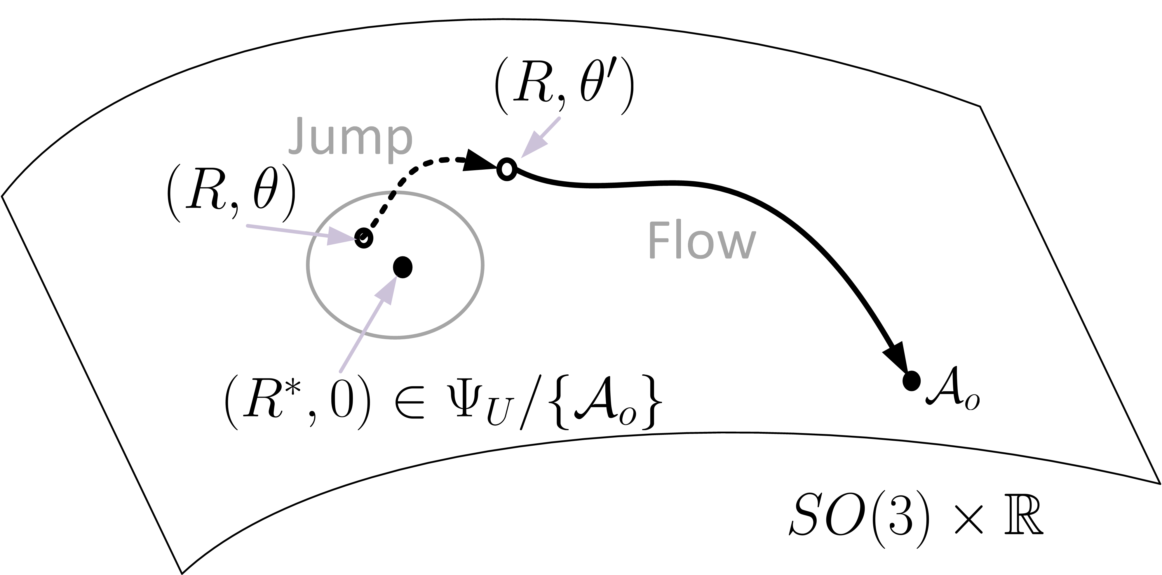
From the definitions of sets and , the set denotes the set of all the undesired critical points of . Assumption 1 implies that for any undesired critical point , there exists another state with such that the value of is lower than the value of by a constant gap . Hence, one can reset (at each jump) to the one leading to the minimum value of with a strict decrease such that the state after jump is away from the undesired critical points. This property, together with an appropriately designed feedback over the flows, will guarantee global asymptotic stability of desired equilibrium point (see an example in Fig. 1). This basic assumption is motivated from the synergistic family of potential functions on proposed in [22, 21, 23].
Once a nonempty finite set and a potential function satisfying the basic Assumption 1 are constructed, as it will be shown later, the flow and jump dynamics governing the evolution of and in turn of will be designed to avoid the undesired critical points, leaving as the unique attractor. In fact, flows when the state is away from the set , and jumps to some leading to minimum value of ) when the state is in the neighborhood of the set . We propose the following hybrid dynamics for :
| (12) |
with . The flow and jump sets are defined as
| (13a) | ||||
| (13b) | ||||
with defined in (11), and the flow map and jump map are defined as
| (14) | ||||
| (15) |
with constant scalar . By Assumption 1, the design of the jump set implies that all the undesired critical points are located in the jump set, i.e., . Note that the flow map in (14) is nothing else but the negative gradient of with respect to contributing to driving the state towards the critical points of . The jump map in (15) is designed to drive (through jumps) the state away from the undesired critical points. From the definitions of the jump set and jump map , it is clear that every , one has , which guarantees a minimum decrease of the potential function by , after each jump.
V Hybrid Feedback Design
We propose the following hybrid feedback tracking control scheme:
| (21) |
where function is defined in (8a), the flow and jump sets and are defined in (13a) and (13b), respectively, the function is given by
| (22) |
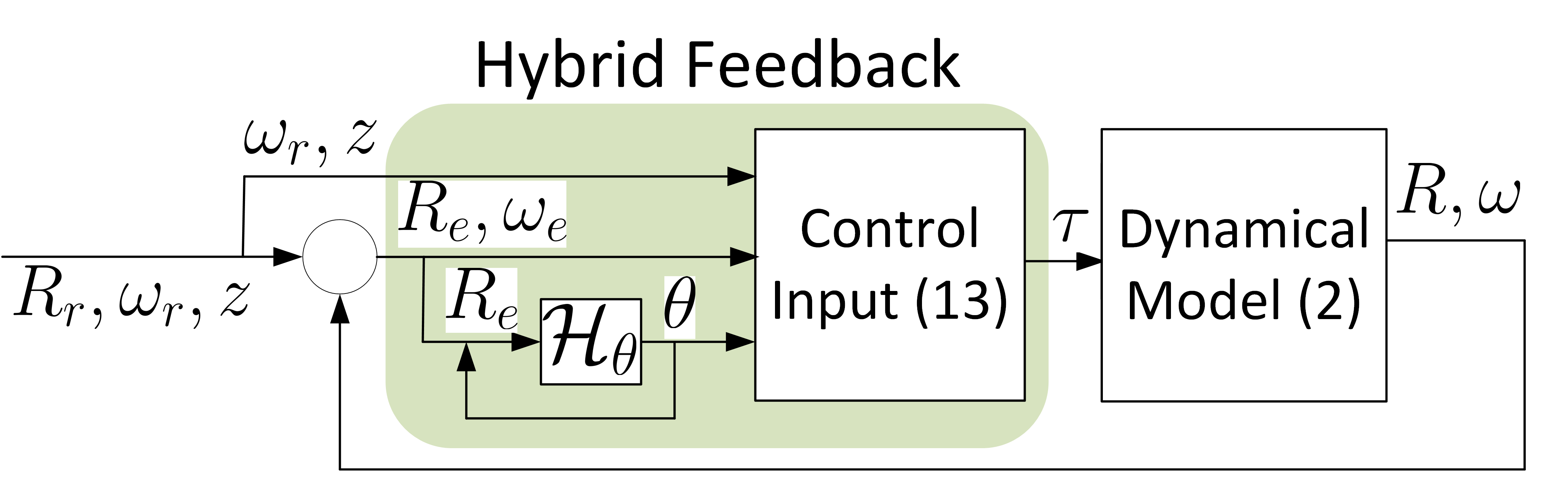
with constant scalars , and the maps and (in terms of and ) are defined in (14) and (15), respectively. The main difference between the proposed hybrid feedback (21)-(22) with respect to the ones proposed in [23, 27] is the extended hybrid dynamics of the auxiliary variable which modifies (continuously) the potential function in the flow set and modifies (through jumps) the potential function in the jump set (i.e., in the neighborhood of the undesired critical points of ). The gradient of the potential function , with the extended hybrid dynamics of , is used in the control to force to be a global attractor. Fig. 2 illustrates the proposed hybrid feedback strategy.
Define the new state space and the new state . In view of (7), (12)-(13) and (21), one has the following hybrid closed-loop system:
| (23) |
where the flow and jump maps are given by
| (24) | ||||
| (25) |
with and defined in (8b), (14), (15) and (22), respectively. One can verify that , and are closed, and the hybrid closed-loop system (23) is autonomous and satisfies the hybrid basic conditions [16, Assumption 6.5]. Now, one can state one of our main results:
Theorem 1.
Proof.
See Appendix -A. ∎
Remark 2.
As shown in the proof of Theorem 1, Assumption 1 is the key to avoid the undesired equilibrium points and ensure GAS for the closed-loop system (23). Without a strict decrease of the potential function over the jumps, the trajectories may converge to a level set containing one of the undesired equilibrium points.
Now, under the following additional assumptions on the potential function , we will show that the proposed hybrid controller achieves exponential stability.
Assumption 2.
Assumption 3.
Assumptions 2 and 3 impose some bounds on the gradients of the potential function and the time derivative of . This assumptions are not very restrictive as it is going to be shown later once we present the construction of the potential function in Section VIII.
Let
. Since is a potential function on with respect to , it follows from the definitions of and that for all , and for all .
Now, one can state the following result:
Proposition 1.
Proof.
See Appendix -B. ∎
Remark 3.
Proposition 1 shows that the tracking error converges exponentially to the set for each initial condition in the compact set satisfying (Note that is compact by assumption). It is important to mention that the exponential stability proved in Proposition 1 is referred to as semi-global exponential stability, since the parameters depend on the initial conditions which are restricted to an arbitrary compact subset . Since the number of jumps is finite, the hybrid exponential stability can be viewed as the exponential stability in the classical sense (exponential convergence over time). This situation is sometimes referred to as exponentially stability in the -direction [35].
VI Hybrid Feedback With Torque Smoothing Mechanism
In order to remove the discontinuities in the control input (caused by the discrete jumps of ), we propose the following modified hybrid feedback tracking scheme:
| (37) |
where , constants , the maps and are defined in (14) and (15), the function is defined in (8a), and the function is given by
| (38) |
with constant . In this case, the flow and jump sets are given by
| (39) | ||||
| (40) |
where , and
| (41) | ||||
| (42) |
with some to be designed later. The main difference between this hybrid control scheme and the previous one in (21), is the use of an dynamical variable that bears the hybrid jumps of resulting in a jump-free control signal. As shown in (37)-(38), the dynamics of allow to relocate the jumps one integrator away from the control torque. This mechanism leads to a continuous torque input since is continuous (not necessary differentiable due to the discrete jumps of in the gradient-based term).
Since is a potential function on with respect to and as , one can show that defined in (42) is a potential function on with respect to , and the set of its critical points is given by . To ensure that all the undesired critical points of are located in the jump set in (40), we consider the following assumption:
Assumption 4.
There exists a constant such that for all .
The proof of Lemma 1 is given in Appendix -C. From the definition of in (40), Lemma 1 implies that all the undesired critical points of in (42) are located in the jump set (i.e., ) under Assumption 1, 4 and some small enough positive constant .
Define the new state space and the new state . In view of (7), (12)-(13) and (37)-(38), one has the following hybrid closed-loop system:
| (44) |
where the flow and jump maps are given by
| (45) | ||||
| (46) |
with and defined in (8b), (14) and (15), respectively. One can verify that , and are closed, and the hybrid closed-loop system (44) satisfies the hybrid basic conditions [16, Assumption 6.5]. The properties of the set for the closed-loop system (44) are stated in the following theorem:
Theorem 2.
Proof.
See Appendix -D. ∎
Following similar steps as in the proof of Proposition 1, one can also show that, under the additional Assumption 2, the proposed hybrid feedback, with the torque smoothing mechanism, guarantees semi-global exponential stability. Note that the high gain condition on in Theorem 2 can be relaxed by considering the following dynamics for :
| (47) |
where with some constants and . With this modification, global asymptotic stability is also guaranteed as in Theorem 2, and the proof is omitted here.
VII Hybrid Feedback Without Velocity Measurements
Inspired by the work in [36, 37, 27], we propose a new hybrid feedback for global attitude tracking without using the measurements of angular velocity . In practice, obviating the need of the angular velocity measurements is of great interest in applications relying on expensive and prone-to-failure gyroscopes. In the case where gyroscopes are available, this velocity-free tracking controller can also be used as a backup scheme triggered by gyro failure.
Consider the auxiliary state and the following hybrid auxiliary system:
| (52) |
where , , the flow and jump sets and are defined in (13a) and (13b), respectively, and is given by
| (53) |
with a symmetric positive definite matrix . The dynamics of the auxiliary variable are inspired from [37, 27], and the maps and are given in (14) and (15), respectively.
We propose the following velocity-free hybrid feedback tracking scheme:
| (59) |
where the hybrid dynamics of the auxiliary state are given in (52), and the function is given by
| (60) |
with constants . The flow and jump sets and are defined in (13a) and (13b), respectively.
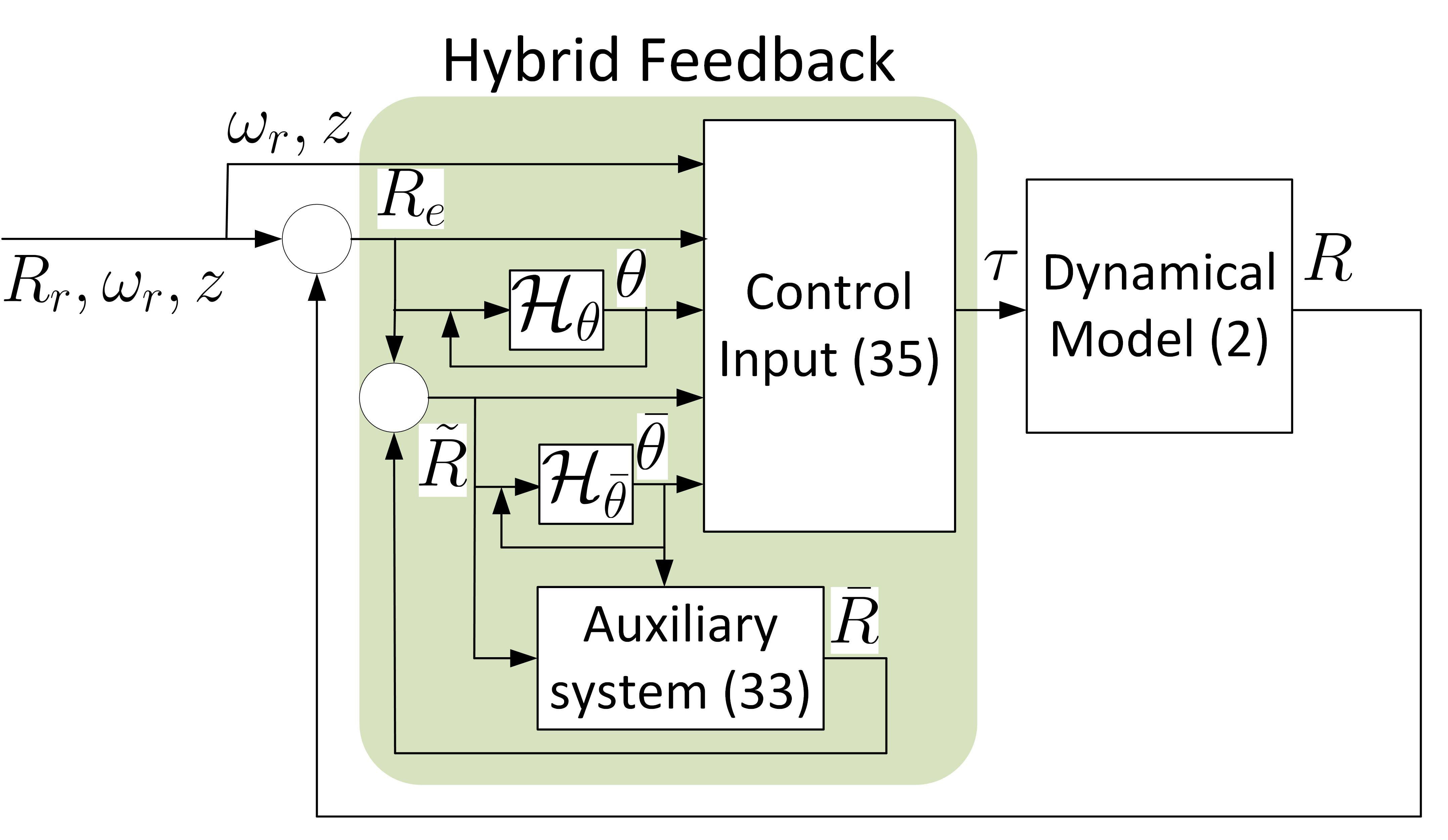
Instead of using the angular velocity tracking error as in the hybrid controllers (21) and (37), a new term generated from the gradient of is considered in the design of the control input in (59). This term, relying on the output of the auxiliary system (52)-(53), allows to generate the necessary damping in the absence of the angular velocity measurements. In fact, an appropriate design of the input of the auxiliary system, ensures the convergence of to as , which consequently leads to and . Fig. 3 illustrates the proposed velocity-free hybrid feedback strategy.
Define the new state space and the new state . In view of (7), (12)-(13) and (52)-(59), one has the following closed-loop system:
| (61) |
where and , and the flow and jump maps are given by
| (62) | ||||
| (63) |
with and defined in (8b), (14) and (15), respectively. The function is defined as: if (i.e., ) otherwise , and the function is defined as: if (i.e., ) otherwise . One can verify that , sets and are closed, and the hybrid system (61) satisfies the hybrid basic conditions [16, Assumption 6.5]. Now, one can state the following result:
Theorem 3.
Proof.
See Appendix -E. ∎
Remark 4.
Following similar steps as in the proof of Proposition 1, one can also show that, under the additional Assumptions 2 and 3, the proposed velocity-free hybrid tracking controller guarantees semi-global exponential stability. Moreover, similar to Section VI, the proposed velocity-free hybrid attitude tracking controller (59) can be further extended with a torque smoothing mechanism by filtering the terms and as in Section VI to obtain a jump-free torque input.
VIII Construction of The Potential Function on
Our proposed designs in the previous sections rely on the existence of a potential function on with respect to , satisfying Assumptions 1-4. In this section, we will provide a systematic procedure for the construction of such potential function using the angular warping techniques inspired by [21].
Consider the following transformation map :
| (64) |
where , is a constant unit vector and is a real-valued variable with hybrid dynamics specified in Section IV. From (64), applies a rotation by an angle to about the unit vector . The main difference compared to the transformation maps considered in [21, 22, 23, 26, 28], is that the angular warping angle considered in (64) is an independent real-valued variable with hybrid flows and jumps.
Consider a modified trace function with being a positive definite matrix. It follows from [23, 38] that the set of all the critical points of is given by with denoting the set of unit eigenvectors of . Let us introduce the following real-valued function on as
| (65) |
with some constant to be designed. The first term of is modified from the potential function inspired by [22, 21], and the second term is a quadratic term in . From the definition of in (64), one can easily verify that for all , and if and only if . Hence, is a potential function on with respect to . The following lemma provides useful properties of the potential function .
Lemma 2.
Let be a positive definite matrix. Consider the potential function defined in (65), and the trajectories generated by and with . Then, for all the following statements hold:
| (66a) | ||||
| (66b) | ||||
| (66c) | ||||
| (66d) | ||||
| (66e) | ||||
where with , and .
Proof.
See Appendix -F. ∎
Remark 5.
Note that in (66a), we obtain a different form of the time derivative of the transformation map on compared to [21, Theorem 6] and [26, Lemma 1]. As mentioned before, the transformation map in [21] and [26] needs to be a (local) diffeomorphism to obtain the new set of critical points of the potential functions after transformation. In our approach, the set of critical points of the potential function on with respect to , denoted by in (66d), can be easily obtained from (66b) and (66c) without any additional conditions. Moreover, from (66d), the set is given by a simple extension of the set with . This property allows us to set the state away from the undesired critical points in by resetting the variable to some non-zero values, which is the key of our reset mechanism proposed in Section IV.
We define the set of parameters with a finite non-empty real-valued set , a matrix , a unit vector , and constant scalars . The following proposition verifies all the conditions in Assumption 1-4 required by Section V-VII.
Proposition 2.
Consider the potential function defined in (65). Then, Assumptions 2-4 hold for any and being positive definite. Moreover, the basic Assumption 1 holds given the set defined as follows:
| (72) |
where scalars and are given as per one of the following three cases:
-
1)
if , and .
-
2)
if , and .
-
3)
if , and
with denoting the -th pair of eigenvalue-eigenvector of matrix .
Proof.
See Appendix -G ∎
Remark 6.
As shown in the proof of Proposition 2, Assumption 1 holds if there exists a unit vector such that one has , where . Proposition 2 provides a design option for the potential function through the choice of the set given in (72). Inspired by [26], the unit vector is designed in terms of the eigenvalues and eigenvectors of the matrix with . The choice of the unit vector in Proposition 2 is optimal in terms of (see [26, Proposition 2] for more details).
Remark 7.
Note that a decrease in the value of results in an increase of the gap (strengthening the robustness to measurement noise). However, it may slow down the convergence of as per (14), leading to lower convergence rates for the overall closed-loop system. Hence, the parameter needs to be carefully chosen via a trade-off between the robustness to measurement noise and the convergence rates of the overall closed-loop system. The performance of the closed-loop system, in terms of convergence rates, with different choices of is illustrated in the simulation section.
IX Extension to Global Pose Tracking on
In this section, we extend our previous hybrid control strategy on to the 3-dimensional Special Euclidean group , defined as
with and denoting the rotation and position, respectively. The Lie algebra of , denoted by , is defined as
with and denoting the angular and linear velocities, respectively. The definitions of the maps , , the adjoint action map and the adjoint operator , and their properties are given in Appendix -H.
We consider the following fully actuated system on
| (73) |
where denotes the pose of a rigid body system, denotes the group velocity, denotes the inertia matrix, and with and denoting the force and torque inputs, respectively. Similar to (6), the desired reference trajectory is generated by the following dynamical system:
| (77) |
where , denotes a compact subset of , and and are the desired pose and group velocity, respectively.
Define the pose tracking error and the group velocity tracking error . From (73)-(77), one obtains the following error dynamics:
| (78a) | ||||
| (78b) | ||||
where the functions and are given by
| (79a) | ||||
| (79b) | ||||
Note that the error dynamics in (78) have similar structure as in (7), and the equality holds. Let be a potential function on with respect to . Hence, given the following smooth gradient-based feedback
| (80) |
the equilibrium point of the closed-loop system (78)-(80) can be shown to be AGAS.
Now, we will illustrate the difficulty of the application of the synergistic hybrid approach on . Applying the “angular-warping” technique from [21] directly on , one has the transformation map as with and . Repeating the results in [21, Theorem 6], one obtains with . To guarantee that is a diffeomorphism as in [21, Theorem 8], one way is to show that matrix is invertible on , i.e., for all . However, the choice of the scalar is difficult due to the fact that is non-compact and the upper bound of cannot be a priori determined. To avoid this issue, an alternative design for hybrid feedback on with GAS guarantees has been proposed in [24], which combines a hybrid attitude feedback relying on a synergistic family of potential functions on and a smooth linear feedback for the vector states. The key of this approach is that it separates the non-compact Lie group into a compact Lie group and a linear space and, as such, the control is designed on rather than on directly. Our approach, however, is not restricted to compact manifolds and can handle the design of geometric hybrid control schemes directly on .
Let be a potential function on with respect to and be a nonempty finite set. We propose the following hybrid feedback tracking scheme:
| (88) |
where , is defined in (79b), the flow map and the jump map are defined as
| (89) | ||||
| (90) |
with , and the flow and jump sets are given as
| (91a) | ||||
| (91b) | ||||
with some and the map given as
| (92) |
The proposed hybrid feedback (88) is modified from (21) and designed on , in terms of the geometric tracking errors and a general potential function on . Now, one can state the following result:
Theorem 4.
Let and suppose that there exist a potential function on with respect to and a nonempty finite set such that with denoting the set of all critical points of and
| (93) |
with some constant and defined in (92). Then, the set is globally asymptotically stable for the closed-loop system (78) with the hybrid feedback (88), and the number of jumps is finite.
The proof of Theorem 4 can be conducted by following the same steps as in the proof of Theorem 1, and therefore is omitted here. It is important to point out that the key condition of Theorem 4 is that the basic Assumption 1 holds for (i.e., inequality (93)). To complete the hybrid feedback design on , we need to construct a potential function on such that inequality (93) holds.
Consider the following transformation map :
| (94) |
where , is a constant vector and is a real-valued variable with hybrid dynamics specified in (88)-(90). For the sake of simplicity, let . Let us introduce the following potential function on with respect to
| (95) |
with a symmetric positive definite matrix and a constant to be designed. Let denote the set of critical points of potential function on , which can be computed as per [30, Lemma 5]. The following proposition provides some useful properties of the potential function on :
X Simulation
In this section, numerical simulations are presented to illustrate the performance of the proposed hybrid feedback controllers. We make use of the HyEQ Toolbox in Matlab [39]. The hybrid controller (21) is referred to as ‘Basic Hybrid’, the hybrid controller with torque smoothing mechanism in (37) is referred to as ‘Smooth Hybrid’, and the velocity-free hybrid controller in (59) is referred to as ‘Velocity-Free Hybrid’. For comparison purposes, we also consider the following classical smooth non-hybrid controller, referred to as ‘Non-Hybrid’:
| (97) |
which is modified from the hybrid controller (21) by taking . The inertia matrix of the system is taken as obtained from a quadrotor UAV in [40]. The reference rotation and angular velocity are generated by (6) with , and . For the set in Proposition 2, we choose with , , , , and as per case 2) in Proposition 2 (i.e., ).
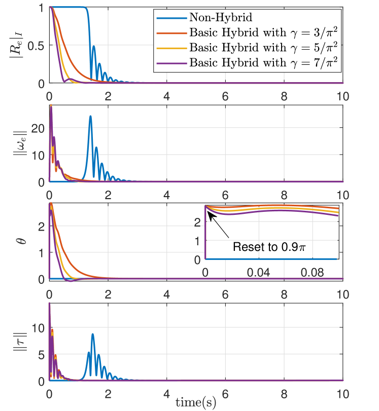
In our first simulation, three different choices of such as are considered in the hybrid controller (21). For each , the constant gap is chosen as . Moreover, the gain parameters are chosen as , and the initial conditions are chosen as , with and , which ensures that initial is close to one of the undesired critical points of . Same gains and initial conditions are considered in the non-hybrid controller (97). The simulation results are given in Fig. 4. As one can see, for the basic hybrid feedback, the variable in (12) jumps from 0 to at and then converges to zero as . Moreover, the tracking errors of both controllers converge to zero as . One can also see that the hybrid controller (21) improves the convergence rate as compared to the non-hybrid controller (97), and an increase in the value of leads to an increase in the convergence rate of the tracking errors.
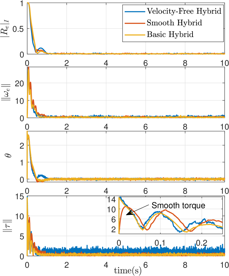
Our second simulation presents a comparison between the three proposed hybrid controllers in the presence of measurements noise. The noisy measurements of attitude and angular velocity are given as with zero-mean Gaussian noise , and with zero-mean Gaussian noise . Same initial conditions for and are chosen as in the previous simulation, and in addition , and are considered. We choose and for , and and for defined in (42). Moreover, the gain parameters are chosen as follows:
|
Note that and are chosen such that . The simulation results are given in Fig. 5. For all controllers, the tracking errors and converge to zero, after one second. Through an appropriate gain tuning, the three hybrid tracking controllers exhibit a quite similar performance. Note that the velocity-free hybrid controller is more sensitive to noise as shown in the plot of the control torque, which is mainly due to the large gain involved in the an auxiliary system (52) to overcome the lack of angular velocity measurements.
XI Conclusion
Three different hybrid feedback control schemes for the attitude tracking problem on , leading to global asymptotic stability, have been proposed. As an instrumental tool in our design, a new potential function on , involving a potential function on and a scalar variable , has been proposed. The scalar variable is governed by hybrid dynamics designed to prevent the extended state in from reaching the undesired critical points, while guaranteeing a decrease of the potential function after each jump. In fact, embedding the manifold in the higher dimensional space allows to modify the critical points on by tying them to . This embedding mechanism provides an easier handling of the critical points on the extended manifold through the hybrid dynamics of the scalar variable .
A global hybrid attitude tracking controller is designed from the gradient of the potential function with the full knowledge of the system state. For practical purposes, two extensions have been proposed: A hybrid attitude tracking controller with jump-free control torque and a velocity-free hybrid attitude tracking controller. The proposed hybrid strategy, involving a single potential function on , on top of being simpler than the existing hybrid approaches involving a synergistic family of potential functions, shows a great potential for other applications involving non-compact manifolds where the synergistic hybrid approaches may not be applicable. This fact has been demonstrated through the design of a globally asymptotically stabilizing (geometric) hybrid feedback for the tracking control problem on the non-compact manifold .
-A Proof of Theorem 1
Consider the following Lyapunov function candidate:
| (98) |
Since is a potential function on with respect to , and is positive definite, one can verify that is positive definite on with respect to . The time derivative of along the flows of (23) is given by
| (99) |
where we used . From (7a) and (12), one obtains
| (100) |
where we made use of the property . Substituting (22) and (100) into (99), one can further show that
| (101) |
for all . Thus, is non-increasing along the flows of (23). Moreover, in view of (23) and (98), for any , one has and
| (102) |
where we made use of the fact for all . Thus, is strictly decreasing over the jumps of (23). From (101) and (102), one concludes that the set is stable as per [15, Theorem 23], and every maximal solution to (23) is bounded. Moreover, in view of (101) and (102), one obtains and for all with . Hence, it is clear that for all , which leads to where denotes the ceiling function. This shows that the number of jumps is finite and depends on the initial conditions.
Next, we will show the global attractivity of . Applying the invariance principle for hybrid systems given in [41, Theorem 4.7], one concludes from (101) and (102) that any solution to the hybrid system (23) must converge to the largest invariant set contained in For each , from one has . It follows from (7b), (21) and (22) that . Using this fact, together with , one can show that with defined in (9). Thus, any solution to the hybrid system (23) must converge to the largest invariant set contained in By Assumption 1, one has and as . It follows from (10) and (13a)-(13b) that and . Then, applying simple set-theoretic arguments, one obtains It follows from and that . Consequently, from the definitions of and , it follows that .
Note that the closed-loop system (23) satisfies the hybrid basic conditions [16, Assumption 6.5], for any with denoting the tangent cone to at the point , , and every maximal solution to (23) is bounded. Therefore, by virtue of [16, Proposition 6.10], it follows that every maximal solution to (23) is complete. Finally, one can conclude that the set is globally asymptotically stable for the hybrid system (23). This completes the proof.
-B Proof of Proposition 1
Consider the following Lyapunov function candidate:
| (103) |
where and is given in (98). From (26), one has , and consequently, one can show that
| (104) |
where matrices and are given as
To guarantee that and are positive definite, it is sufficient to choose .
Since the set is compact by assumption, there exists a constant scalar such that . We define the following compact set It is clear that and . As shown in the proof of Theorem 1, is non-increasing in both flow and jump sets. Hence, for any , one has for all and the number of jumps is bounded by . Using the facts and , it follows that there exist constants such that and for all . Let since is compact by assumption. Hence, from (8b), (22)-(24) and (28), for all one obtains
| (105) |
where , and the following facts , , and , were used.
| (106) |
for all . Let with denoting the -th element of the vector . From (106) and the definition of in (105), one has
To ensure that is positive definite, it is sufficient to choose From (27), one can show that for any , with . Hence, from the definition of and (106), the time derivative of can be rewritten as
| (107) |
Thus, has an exponential decrease over the flows of (23).
On the other hand, from (25), (102) and (103) one obtains
| (108) |
where is chosen as , and we made use of the facts and . Thus, is strictly decreasing over the jumps of (23). Using similar arguments as the ones used at the end of the proof of Theorem 1, it follows that every maximal solution to (23) is complete. In view of (104), (107) and (108), one can show that for all and with and denoting the maximum number of jumps. Letting and making use of (104), one concludes that for all . This completes the proof.
-C Proof of Lemma 1
From the definitions of and , one has and . By Assumption 1, it follows from (10) that for all . In view of the definitions of and in (41)-(42), for any one can show that
| (109) |
where we made use of the facts for all and for all thanks to Assumption 4. By choosing , one concludes (43). This completes the proof.
-D Proof of Theorem 2
Consider the following Lyapunov function candidate:
| (110) |
where in (42) is a potential function on with respect to . For the sake of simplicity, we will use the following notations and . From Assumption 1, it follows that for all . Hence, one can verify that is positive definite on with respect to . In view of (8b), (28), (38) and (45), the time derivative of along the flows of (44) is given by
| (111) |
where and
Similar to the matrix in (106), to guarantee that the matrix is positive definite, it is sufficient to choose Hence, the time derivative of along the flows of (44) can be rewritten as
| (112) |
Thus, is non-increasing along the flows of (44). Moreover, in view of (42)-(44) and (110), for any , one has with , and
| (113) |
where we made use of (43) in Lemma 1. Thus, is strictly decreasing over the jumps of the hybrid system (44). It follows from (112) and (113) that the set is stable as per [15, Theorem 23], and the maximum number of jumps is given by . Moreover, applying the invariance principle in [41, Theorem 4.7], any maximal solution to (44) must converge to the largest invariant set contained in From , one has , which in view of (7b) and (37), implies that . Then, it follows from that . Thus, any solution to (44) must converge to the largest invariant set contained in . Similar to the proof of Theorem 1, applying simple set-theoretic arguments, one obtains and . Moreover, following similar arguments as the ones used at the end of the proof of Theorem 1, one can show that every maximal solution to (44) is complete. Finally, one can conclude that the set is globally asymptotically stable for the hybrid system (44). This completes the proof.
-E Proof of Theorem 3
Consider the following Lyapunov function candidate:
| (114) |
Since is a potential function on , one can verify that is positive definite on with respect to . The time derivative of along the flows of (61) is given by
| (115) |
where we made use of the fact . From (7a) and (52), one obtains . From (12), (14) and (52), one obtains
| (116) |
Substituting (53), (60), (100) and (116) into (115), the time derivative of along the flows of (61) can be rewritten as
| (117) |
for all . Since the matrix is symmetric positive definite, is negative semi-definite in the flow set and is non-increasing along the flows of (61). For any , one obtains if , if , or if . Similar to (102), in view of (61) and (114), one can show that
| (118) |
for all with . Thus, is strictly decreasing over the jumps of (61) on . Similar to the proof of Theorem 1, from (117) and (118) one concludes that the set is stable as per [15, Theorem 23], and the number of jumps is bounded by .
Next, we will show the global attractivity of set . Applying the invariance principle for hybrid systems given in [41, Theorem 4.7], one obtains that every solution to (61) must converge to the largest invariant set contained in For each , it follows that and . Similar to the proof of Theorem 1, one has . From one obtains and . Recall the definition of in (53), it follows from that . From , one has . Since and , it follows from (7b), (59) and (60) that . Using this fact, together with , one can show that . Hence, one verifies that from the definitions of and . Using similar arguments as the ones used at the end of the proof of Theorem 1, it follows that every maximal solution to (61) is complete. Finally, one can conclude that the set is globally asymptotically stable for the hybrid system (61). This completes the proof.
-F Proof of Lemma 2
From (64), the time derivative of the transformation map along the trajectories of and is given by
where we made use of the facts: and . The gradients and can be computed from the differential of in an arbitrary tangential direction , which is given as
| (119) |
where we made use of the property . On the other hand, from (65) and (66a) the time derivative of can be directly obtained as
| (120) |
where we made use of the facts: , and and for all . In view of (119) and (120), one can easily obtain (66b) and (66c).
In view of (66b) and (66c), it follows from and that . Recall the definition of in (64), one can further show that since as . Using the fact , one obtains , which implies that from the definition of the map . Applying [21, Lemma 2], one obtains with denoting the set of eigenvectors of . Using this result, together with , one can conclude that the set of all the critical points of in (11) is given as and , which gives (66d).
-G Proof of Proposition 2
For the sake of simplicity, let . From [29, Lemma 2], one has the following properties for any :
| (122) | ||||
| (123) |
where matrices are symmetric positive definite as matrix is symmetric positive definite, and with denoting the angle between two vectors and denoting the axis of the rotation matrix . Using the facts and , one obtains from (122) that
| (124) |
From (66b) and (124), one can show that Assumption 3 holds by choosing since that for all .
Next, we are going to verify the conditions in Assumption 2. From (65), (66b)-(66c) and (122)-(124), one can show that
| (125) |
where , and we made use of the facts , and . On the other hand, from the definition of in (13a), one has for all . This implies that . Hence, one obtains for all . Letting , it follows from (124) that for all . From (65), (66b)-(66c) and (122)-(124), one can show that
| (126) |
where , and we made use of the facts: , . From the definitions of and using the fact , it is clear that .
Now, we are going to verify the conditions in Assumption 4. Applying the definitions of and , for each one can show that and using the facts: , and for any as per [29, Lemma 2]. It follows from (14) and (66e) that
for all . By choosing and , one can conclude that inequality (28) is satisfied for all .
Finally, we are going to verify the conditions in Assumption 1. From (66d) and , one obtains that . Let be the eigenvalue of associated to the eigenvector . For any and , one can show that
| (127) | ||||
| (128) |
where , and we made use of the facts: , and . Let , and . In view of (11), (127) and (128), for any , one can show that
where we made use of the facts , and for all . Given the set in (72), it follows from [26, Proposition 2] that . This completes the proof.
-H Useful properties on
In this subsection, we first introduce some definitions of the maps , , adjoint action map and adjoint operator . For all with , we define the map as
| (129) |
Motivated by [30], we introduce the following map given as:
| (130) |
with . Similar to the map , one has the following identities:
| (131) | ||||
| (132) |
for all . We define the adjoint operator as
| (133) |
and the adjoint map as
| (134) |
One can also verify the following identities:
| (135a) | ||||
| (135b) | ||||
| (135c) | ||||
| (135d) | ||||
| (135e) | ||||
| (135f) | ||||
for all . Moreover, along the trajectories with , one has
| (136) |
References
- [1] M. Wang and A. Tayebi, “A new hybrid control strategy for the global attitude tracking problem,” in Proc. of the IEEE 58th Conference on Decision and Control (CDC), 2019, pp. 7222–7227.
- [2] P. Crouch, “Spacecraft attitude control and stabilization: Applications of geometric control theory to rigid body models,” IEEE Transactions on Automatic Control, vol. 29, no. 4, pp. 321–331, 1984.
- [3] B. Wie, H. Weiss, and A. Arapostathis, “Quaternion feedback regulator for spacecraft eigenaxis rotations,” AIAA J. Guidance Control, vol. 12, no. 3, pp. 375–380, 1989.
- [4] J.-Y. Wen and K. Kreutz-Delgado, “The attitude control problem,” IEEE Transactions on Automatic Control, vol. 36, no. 10, pp. 1148–1162, 1991.
- [5] K. Y. Pettersen and O. Egeland, “Time-varying exponential stabilization of the position and attitude of an underactuated autonomous underwater vehicle,” IEEE Transactions on Automatic Control, vol. 44, no. 1, pp. 112–115, 1999.
- [6] N. A. Chaturvedi, A. K. Sanyal, and N. H. McClamroch, “Rigid-body attitude control,” IEEE control systems magazine, vol. 31, no. 3, pp. 30–51, 2011.
- [7] R. Naldi, M. Furci, R. G. Sanfelice, and L. Marconi, “Robust global trajectory tracking for underactuated VTOL aerial vehicles using inner-outer loop control paradigms,” IEEE Transactions on Automatic Control, vol. 62, no. 1, pp. 97–112, 2017.
- [8] D. E. Koditschek, “The application of total energy as a Lyapunov function for mechanical control systems,” Contemporary mathematics, vol. 97, pp. 131–157, 1989.
- [9] F. Bullo and R. M. Murray, “Tracking for fully actuated mechanical systems: A geometric framework,” Automatica, vol. 35, no. 1, pp. 17–34, 1999.
- [10] S. P. Bhat and D. S. Bernstein, “A topological obstruction to continuous global stabilization of rotational motion and the unwinding phenomenon,” Systems & Control Letters, vol. 39, no. 1, pp. 63–70, 2000.
- [11] D. S. Maithripala, J. M. Berg, and W. P. Dayawansa, “Almost-global tracking of simple mechanical systems on a general class of Lie groups,” IEEE Transactions on Automatic Control, vol. 51, no. 2, pp. 216–225, 2006.
- [12] T. Lee, “Robust adaptive attitude tracking on SO(3) with an application to a quadrotor UAV,” IEEE Transactions on Control Systems Technology, vol. 21, no. 5, pp. 1924–1930, 2012.
- [13] D. Invernizzi, M. Lovera, and L. Zaccarian, “Dynamic attitude planning for trajectory tracking in thrust-vectoring UAVs,” IEEE Transactions on Automatic Control, vol. 65, no. 1, pp. 453–460, 2020.
- [14] M. Morse, The calculus of variations in the large. American Mathematical Soc., 1934, vol. 18.
- [15] R. Goebel, R. G. Sanfelice, and A. R. Teel, “Hybrid dynamical systems,” IEEE Control Systems, vol. 29, no. 2, pp. 28–93, 2009.
- [16] ——, Hybrid Dynamical Systems: modeling, stability, and robustness. Princeton University Press, 2012.
- [17] C. G. Mayhew, R. G. Sanfelice, and A. R. Teel, “Quaternion-based hybrid control for robust global attitude tracking,” IEEE Transactions on Automatic Control, vol. 56, no. 11, pp. 2555–2566, 2011.
- [18] R. Schlanbusch, E. I. Grøtli, A. Loria, and P. J. Nicklasson, “Hybrid attitude tracking of rigid bodies without angular velocity measurement,” Systems & Control Letters, vol. 61, no. 4, pp. 595–601, 2012.
- [19] R. Schlanbusch and E. I. Grøtli, “Hybrid certainty equivalence control of rigid bodies with quaternion measurements,” IEEE Transactions on Automatic Control, vol. 60, no. 9, pp. 2512–2517, 2014.
- [20] H. Gui and G. Vukovich, “Global finite-time attitude tracking via quaternion feedback,” Systems & Control Letters, vol. 97, pp. 176–183, 2016.
- [21] C. G. Mayhew and A. R. Teel, “Synergistic potential functions for hybrid control of rigid-body attitude,” in Proceedings of American Control Conference (ACC), 2011. IEEE, 2011, pp. 875–880.
- [22] ——, “Hybrid control of rigid-body attitude with synergistic potential functions,” in Proceedings of American Control Conference (ACC), 2011. IEEE, 2011, pp. 287–292.
- [23] ——, “Synergistic hybrid feedback for global rigid-body attitude tracking on SO(3),” IEEE Transactions on Automatic Control, vol. 58, no. 11, pp. 2730–2742, 2013.
- [24] P. Casau, R. G. Sanfelice, R. Cunha, and C. Silvestre, “A globally asymptotically stabilizing trajectory tracking controller for fully actuated rigid bodies using landmark-based information,” International Journal of Robust and Nonlinear Control, vol. 25, no. 18, pp. 3617–3640, 2015.
- [25] T. Lee, “Global exponential attitude tracking controls on SO(3),” IEEE Transactions on Automatic Control, vol. 60, no. 10, p. 2837–2842, 2015.
- [26] S. Berkane and A. Tayebi, “Construction of synergistic potential functions on SO(3) with application to velocity-free hybrid attitude stabilization,” IEEE Transactions on Automatic Control, vol. 62, no. 1, pp. 495–501, 2017.
- [27] S. Berkane, A. Abdessameud, and A. Tayebi, “Hybrid output feedback for attitude tracking on SO(3),” IEEE Transactions on Automatic Control, vol. 63, no. 11, pp. 3956–3963, 2018.
- [28] ——, “Hybrid global exponential stabilization on SO(3),” Automatica, vol. 81, pp. 279–285, 2017.
- [29] ——, “Hybrid attitude and gyro-bias observer design on SO(3),” IEEE Transactions on Automatic Control, vol. 62, no. 11, pp. 6044–6050, 2017.
- [30] M. Wang and A. Tayebi, “Hybrid pose and velocity-bias estimation on SE(3) using inertial and landmark measurements,” IEEE Transactions on Automatic Control, vol. 64, no. 8, pp. 3399–3406, 2019.
- [31] ——, “Hybrid nonlinear observers for inertial navigation using landmark measurements,” IEEE Transactions on Automatic Control, vol. 65, no. 12, pp. 5173–5188, 2020.
- [32] P. Casau, R. Cunha, R. G. Sanfelice, and C. Silvestre, “Hybrid control for robust and global tracking on smooth manifolds,” IEEE Transactions on Automatic Control, vol. 65, no. 5, pp. 1870–1885, 2020.
- [33] A. R. Teel, F. Forni, and L. Zaccarian, “Lyapunov-based sufficient conditions for exponential stability in hybrid systems,” IEEE Transactions on Automatic Control, vol. 58, no. 6, pp. 1591–1596, 2013.
- [34] L. Ljusternik and L. Schnirelmann, Méthodes topologiques dans les problèmes variationnels. Paris, France: Hermann, 1934.
- [35] P. Casau, C. G. Mayhew, R. G. Sanfelice, and C. Silvestre, “Robust global exponential stabilization on the n-dimensional sphere with applications to trajectory tracking for quadrotors,” Automatica, vol. 110, p. 108534, 2019.
- [36] A. Tayebi, “Unit quaternion observer based attitude stabilization of a rigid spacecraft without velocity measurement,” in Proc. of the 45th IEEE Conference on Decision and Control (CDC), 2006, pp. 1557–1561.
- [37] ——, “Unit quaternion-based output feedback for the attitude tracking problem,” IEEE Transactions on Automatic Control, vol. 53, no. 6, pp. 1516–1520, 2008.
- [38] R. Mahony, T. Hamel, and J.-M. Pflimlin, “Nonlinear complementary filters on the special orthogonal group,” IEEE Transactions on automatic control, vol. 53, no. 5, pp. 1203–1218, 2008.
- [39] R. Sanfelice, D. Copp, and P. Nanez, “A toolbox for simulation of hybrid systems in Matlab/Simulink: Hybrid Equations (HyEQ) Toolbox,” in Proc. of the 16th international conference on Hybrid systems: computation and control, 2013, pp. 101–106.
- [40] M. Wang, “Attitude control of a quadrotor UAV: Experimental results:,” Master’s thesis, Lakehead University, 2015.
- [41] R. G. Sanfelice, R. Goebel, and A. R. Teel, “Invariance principles for hybrid systems with connections to detectability and asymptotic stability,” IEEE Transactions on Automatic Control, vol. 52, no. 12, pp. 2282–2297, 2007.