Hybrid explicit-implicit learning for multiscale problems with time dependent source
Abstract
The splitting method is a powerful method for solving partial differential equations. Various splitting methods have been designed to separate different physics, nonlinearities, and so on. Recently, a new splitting approach has been proposed where some degrees of freedom are handled implicitly while other degrees of freedom are handled explicitly. As a result, the scheme contains two equations, one implicit and the other explicit. The stability of this approach has been studied. It was shown that the time step scales as the coarse spatial mesh size, which can provide a significant computational advantage. However, the implicit solution part can be expensive, especially for nonlinear problems. In this paper, we introduce modified partial machine learning algorithms to replace the implicit solution part of the algorithm. These algorithms are first introduced in ‘HEI: Hybrid Explicit-Implicit Learning For Multiscale Problems’, where a homogeneous source term is considered along with the Transformer, which is a neural network that can predict future dynamics. In this paper, we consider time-dependent source terms which is a generalization of the previous work. Moreover, we use the whole history of the solution to train the network. As the implicit part of the equations is more complicated to solve, we design a neural network to predict it based on training. Furthermore, we compute the explicit part of the solution using our splitting strategy. In addition, we use Proper Orthogonal Decomposition based model reduction in machine learning. The machine learning algorithms provide computational saving without sacrificing accuracy. We present three numerical examples which show that our machine learning scheme is stable and accurate.
1 Introduction
Many physical problems vary at multiple space and time scales. The solutions of these problems are difficult to compute as we need to resolve the time and space scales. For example, porous media flow and transport occur over many space and time scales. Many multiscale and splitting algorithms have been proposed to solve these problems [28, 18, 41]. In this paper, we would like to combine machine learning and splitting/multiscale approaches to predict the dynamics of complex forward problems. Our goal is to perform machine learning on a small part of the solution space, while computing “the rest” of the solution fast. Our proposed splitting algorithms allow doing it, which we will describe below.
Our approaches use multiscale methods in their construction to achieve coarser time stepping. Multiscale methods have extensively been studied in the literature. For linear problems, homogenization-based approaches [23, 39, 40], multiscale finite element methods [23, 31, 35], generalized multiscale finite element methods (GMsFEM) [12, 13, 14, 17, 21], Constraint Energy Minimizing GMsFEM (CEM-GMsFEM) [15, 16, 7], nonlocal multi-continua (NLMC) approaches [19], metric-based upscaling [44], heterogeneous multiscale method [20], localized orthogonal decomposition (LOD) [30], equation-free approaches [45, 46], multiscale stochastic approaches [33, 34, 32], and hierarchical multiscale methods [5] have been studied. Approaches such as GMsFEM and NLMC are designed to handle high-contrast problems. For nonlinear problems, we can replace linear multiscale basis functions with nonlinear maps [26, 27, 22].
Splitting methods are introduced when solving dynamic problems [3, 47, 29]. There is a wide range of applications for splitting methods, e.g. splitting physics, scales, and so on. Splitting methods allow simplifying the large-scale problem into smaller-scale problems. We couple them and obtain the final solution after we solve the smaller-scale problems. Recently, a partially explicit splitting method [28, 18, 24] is proposed for linear and nonlinear multiscale problems. In this approach, we treat some solution parts implicitly while treating the other parts explicitly. The stability analysis shows that the time step only depends on the explicit part of the solution. With the careful splitting of the space, we are able to make the time step scale as the coarse mesh size and independent of contrast.
To illustrate the main idea of our methods, we consider
In this paper, we combine machine learning and splitting approaches (such as the partially explicit method). In the splitting algorithm, we write the solution as , where is computed implicitly and is computed explicitly. In our previous work, the Transformer has been used to solve this kind of problem in [25, 11]. In [25], we consider zero source term and use the Transformer to predict the future dynamics of the solution. In our current paper, we consider full dynamics and time-dependent source terms. The latter occurs in porous media applications and represents the rates of wells, which vary in time. The goal in these simulations is to compute the solutions at all time steps for a given time-dependent source term in an efficient way, which is not addressed before.
Many machine learning and multiscale methods are designed for solving multiscale parametric PDEs [11, 48, 49, 9, 43, 42]. The advantage of machine learning is that it treats PDEs as an input-to-output map. By training, and possibly, using the observed data, machine learning avoids computing solutions for each input (such as parameters in boundary conditions, permeability fields or sources). In this paper, we use machine learning to learn the difficult-to-compute part of the solution that is, in general, computed implicitly. This is a coarse-grid part of the solution, which can also be observed given some dynamic data. The splitting algorithm gives two coupled equations. The first equation for is implicit while the second equation for is explicit. We design a neural network to predict the first component of the solution. Then, we calculate the second component using the discretized equations. The inputs of our neural network are the parameters that characterize the source term of the equation. The outputs are the whole history of , i.e. at all time steps. The output dimension of our neural network is the dimension of times the number of time steps, which is considerably large. Therefore, we use Proper Orthogonal Decomposition (POD) [48, 10, 38] to reduce the dimension of the solution space. We concatenate all solution vectors of every training input together to generate a large-scale matrix. After doing the singular value decomposition, we select several dominant eigenvectors to form the POD basis vectors. Thus, the output becomes the coordinate vectors based on the POD basis vectors and its dimension is greatly reduced, so is the number of parameters inside the neural networks.
In this paper, we show several numerical examples to illustrate our learning framework which is based on the partially explicit scheme. In our numerical examples, the diffusion term is and the reaction term is . is a source term that is nonzero on several coarse blocks and is zero elsewhere. We choose such as it simulates the wells in petroleum applications. By comparing with the solution which is obtained using fine grid basis functions, we find that the relative error is small and similar to the scheme where we calculate both components. Thus, the learning scheme can achieve similar accuracy while saving computation.
2 Problem Setting
We consider the following parabolic partial differential equation
| (2.1) |
Let be a Hilbert space. In this equation, with being the variational derivative of energy . In this paper, we use to denote for simplicity. We assume that is contrast dependent (linear or nonlinear). Here, is a time dependent source term with parameters. The weak formulation of Equation (2.1) is the following. We want to find such that
| (2.2) |
The is the inner product. We assume that
| (2.3) |
Example 1.
The standard approach to solving this problem is the finite element method. Let be the finite element space and is the numerical solution satisfying
| (2.4) |
The Backward Euler (implicit) time discretization for this Equation is
| (2.5) |
The Forward Euler (explicit) time discretization for Equation (2.4) is
| (2.6) |
One can find details about the stability analysis of the Backward and Forward Euler method in [18].
2.1 Partially Explicit Scheme
In this paper, we use the partially explicit splitting scheme introduced in [18]. We split the space to be the direct sum of two subspaces and , i.e. . Then the solution with and satisfies
We use the partially explicit time discretization for this problem. Namely, we consider finding (with ) such that
| (2.7) | |||
| (2.8) |
We refer to [28, 18] for the details of convergence assumptions and stability analysis of the above scheme.
2.1.1 Construction of and
In this section, we present how to construct the two subspaces for our partially explicit splitting scheme. We will first present the CEM method which is used to construct . Next, with the application of eigenvalue problems, we build . In the following discussion, let and then we define .
CEM method
We introduce the CEM finite element method in this section. Let be a coarse grid partition of . For , we need to construct a collection of auxiliary basis functions in . We assume that are basis functions that form a partition of unity, e.g., piecewise linear functions, see [4]. We first find and such that the following equation holds:
where
With rearrangement if necessary, we select the eigenfunctions of the corresponding first smallest eigenvalues. We define
Define a projection operator
with and being the number of coarse elements. We denote an oversampling domain which is several coarse blocks larger than as [15]. For every auxiliary basis , we solve the following two equations and find and
Then we can define the CEM finite element space as
We define and we will need it when we construct in the next subsection.
Construction of
We build the second subspace based on and . Similarly, we first have to construct the auxiliary basis functions by solving the eigenvalue equations. For every coarse element , we search for such that
| (2.9) |
We choose the eigenfunctions corresponding to the smallest eigenvalues. The second type of auxiliary space is defined as . For every auxiliary basis , we look for a basis function such that for some , , we have
| (2.10) | ||||
| (2.11) | ||||
| (2.12) |
We define
3 Machine Learning Approach
In Equation (2.1), we consider as a source term with varying parameters representing temporal changes. For every parameter, we want to find the corresponding solution . For the traditional finite element methods, we need to construct meshes and basis functions, assemble the stiffness and mass matrices and solve the matrices equations, which makes the computation cost large, especially for the nonlinear PDEs as we have to assemble the stiffness matrix at every time step. Designing machine learning algorithms for the partially explicit scheme can alleviate this problem. Once the neural network is trained, the computation of solution becomes the multiplication of matrices and applying activation functions, which is more efficient in contrast to the finite element methods.
The Equation (2.7) is implicit for , which makes the computations more complicated. We design a machine learning algorithm to predict and then we compute using Equation (2.8).
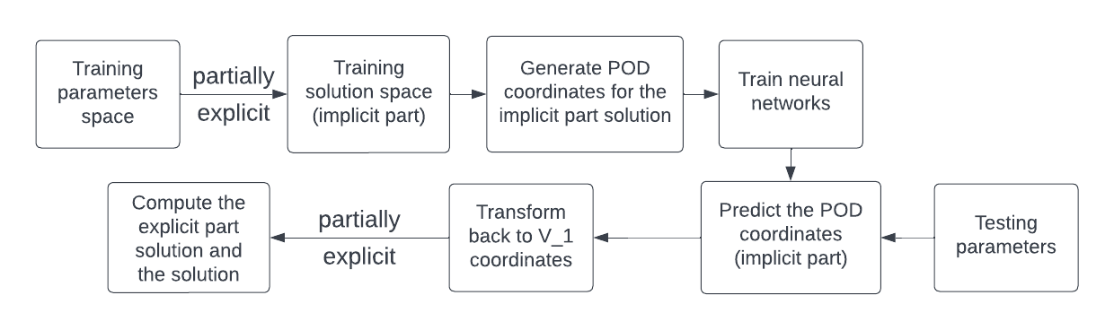
We present a flowchart in Figure 3.1 to show the workflow of our method. We first need to generate the dataset which will be used to train the neural network. Let be the parameters in . We set for with and being the lower bound and upper bound, respectively. We generate the training space by drawing samples from a uniform distribution over the interval . For every in the training space, we calculate its corresponding partially explicit solution using Equations (2.7) and (2.8). Let be the number of time steps and be the size of our training sample space. We denote this solution space as , where . We remark that the reason why starts from is that we need and to compute in the partially explicit scheme. The is computed by the Backward Euler scheme using basis functions from both and . We only need for our machine learning algorithm. Before we move on, we discuss a useful tool called Proper Orthogonal Decomposition [6].
For a given set of vectors with , we want to construct a smaller dimensional vector space that can represent the space spanned by accurately, i.e., we want to find orthonormal vectors that solve
| (3.1) |
where and is the rank of . We apply the singular value decomposition for this. Next, we briefly remind the POD procedure [6]. We first define a matrix whose dimension is . Then and are and dimensional matrices. Consider the eigenvalues and eigenvectors of as well as ,
Next, we define
We now have
where is the diagonal matrix whose main diagonal entries are . After doing rearrangement if necessary, we may assume
The solution of (3.1) is given by the eigenvectors of corresponding to the largest eigenvalues. Thus, the desired dimensional subspace is the subspace spanned by eigenvectors corresponding to the largest eigenvalues.
There are column vectors () in the solution space . We would like to output the solution at the same time so that we don’t have to do the iteration for every time step recursively. In this case, the output dimension is , which is too large ( is in our examples). As a result, the number of parameters in the neural network will also be large, which increases the computation cost. We define
Hence, . After the singular value decomposition to , we define
where is the eigenvector corresponding to the -th largest eigenvalue. We use to get a reduced dimensional coordinate vectors for every ,i.e.
| (3.2) |
Thus, the output dimension is reduced to . In the testing stage, after we get the output , we use to get the coarse grid solution .
As discussed above, in our neural networks, the inputs are the parameters in and outputs are . That is
where is the neural network. To better illustrate,
where , , , and are the output of the first layer, the activation function, inputs, weight matrix and the biased term. Here, , and are row vectors. Similarly,
and
where is the number of layers and . Then, we can obtain by reshaping .
Next, we would like to prove two theoretical results. Under the setting in Section 3, we first define the map from the input to the output of our neural network as
where is a compact subset of with norm . We will show that the neural network is capable of approximating precisely. We then show that when the loss function (mean squared error) goes to zero, the output of the neural network converges to the exact solution (which is computed via the partially explicit scheme). We state the following well-known theorem [36].
Theorem 3.1.
Universal Approximation Theorem. Let be any non-affine continuous function. Also, is continuously differentiable at at least one point and with nonzero derivative at that point. Let be the space of neural networks with inputs, outputs, as the activation function for every hidden layers and the identity function as the activation function for the output layers. Then given any and any function , there exists such that
The universal approximation theorem relies on the continuity assumption of the mapping . More specifically, to apply the universal approximation theorem, we now need to show that is continuous.
Lemma 3.1.
We define and assume is linear. We know . The two subspaces and are finite dimensional subspaces with trivial intersection. By the strengthened Cauchy Schwarz inequality [2], there exists a constant depending on and such that
| (3.3) |
If
| (3.4) |
then is continuous with respect to .
The proof is given in Appendix A. With the continuity of , we have the following theorem.
Theorem 3.2.
For any , there exists such that
The theorem follows from the continuity of and the Universal Approximation Theorem. Finally, we present the estimation of the generalization error.
Theorem 3.3.
Let be the set containing all training samples. Fix . The functions and are uniformly continuous since they are continuous and is compact. It follows that there exists such that
for any and . We assume that for any , there exists such that . Let be the mapping in Theorem 3.2. Then we have
Proof.
For any , we can find such that , it follows that:
As and are arbitrary, we obtain the conclusion. ∎
4 Numerical Results
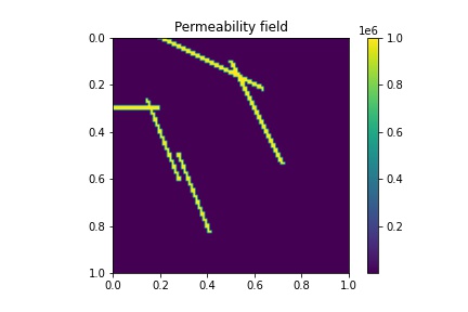
In this section, we present numerical examples. In all cases, the domain is . The permeability field we use is shown in Figure 4.1. Note that there are high contrast channels in the permeability field. The fine mesh size is and the coarse mesh size is .
We define the following notation.
-
•
is obtained by predicting and computing by Equation (2.8).
- •
-
•
is obtained using the fine grid basis functions and Equation (2.5).
We also need to define the following relative error for better illustration. Let be the norm. We know that and .
-
•
, .
-
•
, .
and are used to measure the difference of accuracy between our learning scheme and the scheme in which we compute both and . and are defined to measure how close the learning output is to their target. The neural network is fully connected and is activated by the scaled exponential linear unit (SELU). To obtain the solution of the minimization problem, we use the gradient-based optimizer Adam [37]. The loss function we use is the mean square error (MSE). Our machine learning algorithm is implemented using the open-source library Keras [8] with the Tensorflow [1] backend. The neural network we use is a simple neural network with fully connected layers. We remark that with this neural network, we can obtain high accuracy.
In the first two examples, we consider the following linear parabolic partial differential equations
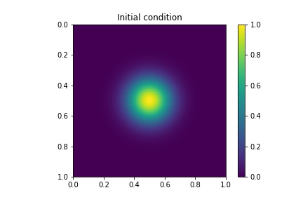
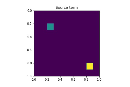
where is the outward normal vector and is the initial condition which is presented it in Figure 4.2. In our first example, the source term is defined as follows,
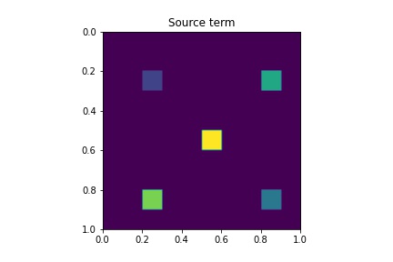
where are parameters. In this case, we let for . We show a simple sketch of in Figure 4.2 to illustrate. This sketch only shows the position of the coarse blocks where the source term is nonzero. We choose this source, which has some similarities to the wells in petroleum engineering. The final time is , there are time steps and the time step size is .
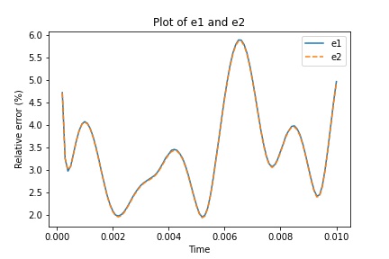
The training space contains samples and the testing space contains samples. Every sample’s parameter is drawn from the uniform distribution over . The number of POD basis vectors is . We choose this based on the eigenvalue behavior in the process of singular value decomposition. We present and defined before in Figure 4.3. The error is calculated at each time step as the average over all samples in the testing space. From the plot in Figure 4.3, we find that the curves for and coincide, which means our learning algorithms can obtain similar accuracy as the scheme in which we compute by Equation (2.7) and (2.8). The average of and over time are and , respectively, which means the output of our learning scheme nearly resembles the corresponding target (the solution we obtain by computing both equations).
In the next case, we test our algorithms using a more complicated source term with more parameters. The source term we use is,
where are parameters. In this case, the parameters of every sample are drawn from the uniform distribution over . We present an easy sketch of in Figure 4.4 to illustrate the positions of the sources. The initial condition is also shown in Figure 4.4. The final time , the number of time steps and the time step size are , and , respectively.

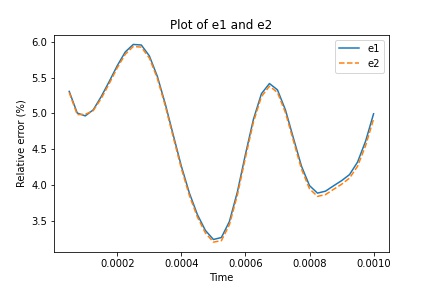
The model is trained using 2000 samples and we test it with 1000 samples. The number of POD basis vectors is . In Figure 4.5, the and are presented. By observing the error plot, we find that and are close to each other, which implies that our learning algorithms can obtain similar accuracy as the scheme where we calculate both and using Equation (2.7) and (2.8). The average of and over time are and , respectively. Such small and indicate that the prediction is accurate.
In the next case, we consider the following equation
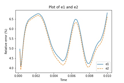
where is the outward normal vector. This equation is nonlinear and its computation cost is much larger than the linear case because we have to assemble the stiffness matrix at every time step. We use the same initial condition and source term as the second example. The final time is , the number of time steps is and the time step size is . We train our neural network using samples and the network is tested using samples. In Figure 4.6, we present and defined before. From the first plot, we find that the curves for and nearly coincide, which implies that our machine learning algorithms can have the same accuracy as we compute the solution by Equations (2.7) and (2.8). The average of and over time are and , respectively, which means our neural network can approximate the target well and achieve a fantastic accuracy.
5 Conclusion
In this paper, we construct neural networks based on the partially explicit splitting scheme. We predict , the implicit part of the solution, while solving for , the explicit part of the solution. The output dimension resulting from is large and we apply the POD to reduce the dimension. The POD transformation greatly reduces the output dimension and at the same time the number of parameters in the neural networks. The POD error is small compared to the overall error. We discuss three numerical examples. We present a theoretical justification. We conclude that our machine learning algorithms can obtain similar accuracy as the partially explicit scheme.
Appendix A Proof of Lemma 3.1
In this section, we prove the Lemma 3.1, i.e., the function
is continuous. We equip with the norm. Let us decompose the mapping as , where
and is the POD transformation defined by (3.2). The map is a projection, thus continuous. We assume that is continuous with respect to and therefore, is continuous. To show that is continuous, we only need to prove is continuous. The proof is given in the next lemma.
Lemma A.1.
Let us assume is linear, and we define a bilinear form and its co-responding norm as . If
| (A.1) |
the function is continuous with respect to the source term .
Proof.
Case I. The solution for is continuous with respect to the source term .
The initial condition is given and the solution at time step is calculated via the fully implicit scheme. Thus, we want to show the continuity from the source term to the solution of the following scheme
where .
In the following proof, we abbreviate the subscript for simplicity.
Let and be different, and let us denote the corresponding sources as and . The discretized solutions and evolved for one time step then satisfy:
It follows immediately that,
Test with , the linearity of then yields,
After rearrangement, we have
Thus,
| (A.2) |
Case II. The solution is continuous with respect to the source term , for .
In the partially explicit scheme, for the source term , the solution satisfies
| (A.3) | |||
| (A.4) |
Similarly, for , the solution satisfies
| (A.5) | |||
| (A.6) |
Let us denote for , and subtract (A.5) from (A.3) and (A.6) from (A.4), it follows that,
The linearity of then yields,
Let and . We get
Sum up these two equations, we have
| (A.7) |
where . The second term of (A.7) on the left hand side can be further estimated as,
where we apply the strenthened Cauchy Schwartz inequality. It follows that,
Note that , we then can estimate the third term of (A.7),
Now (A.7) can be estimated as:
After rearranging, we have
We assume the CFL condition (A.1), specifically,
This yields,
| (A.8) | ||||
where we use (A.2) in the last inequality. Then,
where we apply (A.2) in the last inequality.
With these two inequalities, we can obtain the conclusion.
∎
References
- [1] M. Abadi, A. Agarwal, P. Barham, E. Brevdo, Z. Chen, C. Citro, G. S. Corrado, A. Davis, J. Dean, M. Devin, S. Ghemawat, I. Goodfellow, A. Harp, G. Irving, M. Isard, Y. Jia, R. Jozefowicz, L. Kaiser, M. Kudlur, J. Levenberg, D. Mané, R. Monga, S. Moore, D. Murray, C. Olah, M. Schuster, J. Shlens, B. Steiner, I. Sutskever, K. Talwar, P. Tucker, V. Vanhoucke, V. Vasudevan, F. Viégas, O. Vinyals, P. Warden, M. Wattenberg, M. Wicke, Y. Yu, and X. Zheng. TensorFlow: Large-scale machine learning on heterogeneous systems, 2015. Software available from tensorflow.org.
- [2] J. Aldaz. Strengthened Cauchy-Schwarz and Hölder inequalities. arXiv preprint arXiv:1302.2254, 2013.
- [3] U. M. Ascher, S. J. Ruuth, and R. J. Spiteri. Implicit-explicit Runge-Kutta methods for time-dependent partial differential equations. Applied Numerical Mathematics, 25(2-3):151–167, 1997.
- [4] I. Babuška and J. M. Melenk. The partition of unity method. Int. J. Numer. Meth. Engrg., 40:727–758, 1997.
- [5] D. L. Brown, Y. Efendiev, and V. H. Hoang. An efficient hierarchical multiscale finite element method for stokes equations in slowly varying media. Multiscale Modeling & Simulation, 11(1):30–58, 2013.
- [6] A. Chatterjee. An introduction to the proper orthogonal decomposition. Current Science, 78(7):808–817, 2000.
- [7] B. Chetverushkin, E. Chung, Y. Efendiev, S.-M. Pun, and Z. Zhang. Computational multiscale methods for quasi-gas dynamic equations. Journal of Computational Physics, 440:110352, 2021.
- [8] F. Chollet et al. Keras, 2015.
- [9] E. Chung, Y. Efendiev, W. T. Leung, S.-M. Pun, and Z. Zhang. Multi-agent reinforcement learning accelerated mcmc on multiscale inversion problem. arXiv preprint arXiv:2011.08954, 2020.
- [10] E. Chung, Y. Efendiev, S.-M. Pun, and Z. Zhang. Computational multiscale methods for parabolic wave approximations in heterogeneous media. arXiv preprint arXiv:2104.02283, 2021.
- [11] E. Chung, W. T. Leung, S.-M. Pun, and Z. Zhang. A multi-stage deep learning based algorithm for multiscale model reduction. Journal of Computational and Applied Mathematics, 394:113506, 2021.
- [12] E. T. Chung, Y. Efendiev, and T. Hou. Adaptive multiscale model reduction with generalized multiscale finite element methods. Journal of Computational Physics, 320:69–95, 2016.
- [13] E. T. Chung, Y. Efendiev, and C. Lee. Mixed generalized multiscale finite element methods and applications. SIAM Multiscale Model. Simul., 13:338–366, 2014.
- [14] E. T. Chung, Y. Efendiev, and W. T. Leung. Generalized multiscale finite element methods for wave propagation in heterogeneous media. Multiscale Modeling & Simulation, 12(4):1691–1721, 2014.
- [15] E. T. Chung, Y. Efendiev, and W. T. Leung. Constraint energy minimizing generalized multiscale finite element method. Computer Methods in Applied Mechanics and Engineering, 339:298–319, 2018.
- [16] E. T. Chung, Y. Efendiev, and W. T. Leung. Constraint energy minimizing generalized multiscale finite element method in the mixed formulation. Computational Geosciences, 22(3):677–693, 2018.
- [17] E. T. Chung, Y. Efendiev, and W. T. Leung. Fast online generalized multiscale finite element method using constraint energy minimization. Journal of Computational Physics, 355:450–463, 2018.
- [18] E. T. Chung, Y. Efendiev, W. T. Leung, and W. Li. Contrast-independent partially explicit time discretizations for nonlinear multiscale problems, 2021.
- [19] E. T. Chung, Y. Efendiev, W. T. Leung, M. Vasilyeva, and Y. Wang. Non-local multi-continua upscaling for flows in heterogeneous fractured media. Journal of Computational Physics, 372:22–34, 2018.
- [20] W. E and B. Engquist. Heterogeneous multiscale methods. Comm. Math. Sci., 1(1):87–132, 2003.
- [21] Y. Efendiev, J. Galvis, and T. Hou. Generalized multiscale finite element methods (GMsFEM). Journal of Computational Physics, 251:116–135, 2013.
- [22] Y. Efendiev, J. Galvis, G. Li, and M. Presho. Generalized multiscale finite element methods. nonlinear elliptic equations. Communications in Computational Physics, 15(3):733–755, 2014.
- [23] Y. Efendiev and T. Hou. Multiscale Finite Element Methods: Theory and Applications, volume 4 of Surveys and Tutorials in the Applied Mathematical Sciences. Springer, New York, 2009.
- [24] Y. Efendiev, W. T. Leung, W. Li, S.-M. Pun, and P. N. Vabishchevich. Nonlocal transport equations in multiscale media. modeling, dememorization, and discretizations, 2022.
- [25] Y. Efendiev, W. T. Leung, G. Lin, and Z. Zhang. Hei: hybrid explicit-implicit learning for multiscale problems, 2021.
- [26] Y. Efendiev and A. Pankov. Numerical homogenization of monotone elliptic operators. SIAM J. Multiscale Modeling and Simulation, 2(1):62–79, 2003.
- [27] Y. Efendiev and A. Pankov. Homogenization of nonlinear random parabolic operators. Advances in Differential Equations, 10(11):1235–1260, 2005.
- [28] W. T. L. Eric Chung, Yalchin Efendiev and P. N. Vabishchevich. Contrast-independent partially explicit time discretizations for multiscale flow problems. arXiv:2101.04863.
- [29] J. Frank, W. Hundsdorfer, and J. Verwer. On the stability of implicit-explicit linear multistep methods. Applied Numerical Mathematics, 25(2-3):193–205, 1997.
- [30] P. Henning, A. Målqvist, and D. Peterseim. A localized orthogonal decomposition method for semi-linear elliptic problems. ESAIM: Mathematical Modelling and Numerical Analysis, 48(5):1331–1349, 2014.
- [31] T. Hou and X. Wu. A multiscale finite element method for elliptic problems in composite materials and porous media. J. Comput. Phys., 134:169–189, 1997.
- [32] T. Y. Hou, D. Huang, K. C. Lam, and P. Zhang. An adaptive fast solver for a general class of positive definite matrices via energy decomposition. Multiscale Modeling & Simulation, 16(2):615–678, 2018.
- [33] T. Y. Hou, Q. Li, and P. Zhang. Exploring the locally low dimensional structure in solving random elliptic pdes. Multiscale Modeling & Simulation, 15(2):661–695, 2017.
- [34] T. Y. Hou, D. Ma, and Z. Zhang. A model reduction method for multiscale elliptic pdes with random coefficients using an optimization approach. Multiscale Modeling & Simulation, 17(2):826–853, 2019.
- [35] P. Jenny, S. Lee, and H. Tchelepi. Multi-scale finite volume method for elliptic problems in subsurface flow simulation. J. Comput. Phys., 187:47–67, 2003.
- [36] P. Kidger and T. Lyons. Universal Approximation with Deep Narrow Networks. In J. Abernethy and S. Agarwal, editors, Proceedings of Thirty Third Conference on Learning Theory, volume 125 of Proceedings of Machine Learning Research, pages 2306–2327. PMLR, 09–12 Jul 2020.
- [37] D. P. Kingma and J. Ba. Adam: A method for stochastic optimization, 2017.
- [38] K. Kunisch and S. Volkwein. Galerkin proper orthogonal decomposition methods for parabolic problems. Numerische Mathematik, 90:117–148, 2001.
- [39] C. Le Bris, F. Legoll, and A. Lozinski. An MsFEM type approach for perforated domains. Multiscale Modeling & Simulation, 12(3):1046–1077, 2014.
- [40] W. T. Leung, G. Lin, and Z. Zhang. Nh-pinn: Neural homogenization based physics-informed neural network for multiscale problems. arXiv preprint arXiv:2108.12942, 2021.
- [41] W. Li, A. Alikhanov, Y. Efendiev, and W. T. Leung. Partially explicit time discretization for nonlinear time fractional diffusion equations. arXiv preprint arXiv:2110.13248, 2021.
- [42] G. Lin, C. Moya, and Z. Zhang. Accelerated replica exchange stochastic gradient langevin diffusion enhanced bayesian deeponet for solving noisy parametric pdes. arXiv preprint arXiv:2111.02484, 2021.
- [43] G. Lin, Y. Wang, and Z. Zhang. Multi-variance replica exchange stochastic gradient mcmc for inverse and forward bayesian physics-informed neural network. arXiv preprint arXiv:2107.06330, 2021.
- [44] H. Owhadi and L. Zhang. Metric-based upscaling. Comm. Pure. Appl. Math., 60:675–723, 2007.
- [45] A. Roberts and I. Kevrekidis. General tooth boundary conditions for equation free modeling. SIAM J. Sci. Comput., 29(4):1495–1510, 2007.
- [46] G. Samaey, I. Kevrekidis, and D. Roose. Patch dynamics with buffers for homogenization problems. J. Comput. Phys., 213(1):264–287, 2006.
- [47] H. Shi and Y. Li. Local discontinuous galerkin methods with implicit-explicit multistep time-marching for solving the nonlinear cahn-hilliard equation. Journal of Computational Physics, 394:719–731, 2019.
- [48] Y. Yang, M. Ghasemi, E. Gildin, Y. Efendiev, and V. Calo. Fast Multiscale Reservoir Simulations With POD-DEIM Model Reduction. SPE Journal, 21(06):2141–2154, 06 2016.
- [49] Z. Zhang, E. T. Chung, Y. Efendiev, and W. T. Leung. Learning algorithms for coarsening uncertainty space and applications to multiscale simulations. Mathematics, 8(5):720, 2020.