Hybrid Attention Model Using Feature Decomposition and Knowledge Distillation for Glucose Forecasting
Abstract.
The availability of continuous glucose monitors (CGMs) as over-the-counter commodities have created a unique opportunity to monitor a person’s blood glucose levels, forecast blood glucose trajectories, and provide automated interventions to prevent devastating chronic complications that arise from poor glucose control. However, forecasting blood glucose levels (BGL) is challenging because blood glucose changes consistently in response to food intake, medication intake, physical activity, sleep, and stress. It is particularly difficult to accurately predict BGL from multimodal and irregularly sampled data and over long prediction horizons. Furthermore, these forecasting models need to operate in real-time on edge devices to provide in-the-moment interventions. To address these challenges, we propose GlucoNet 111Code base is available here: https://github.com/shovito66/GlucoNet, an AI-powered sensor system for continuous monitoring of behavioral and physiological health and robust forecasting of blood glucose patterns. GlucoNet devises a feature decomposition-based lightweight transformer model that incorporates patients’ behavioral and physiological data (e.g., blood glucose, diet, medication) and transforms sparse and irregular patient data (e.g., diet and medication intake data) into continuous features using a mathematical model, facilitating better integration with the BGL data. Given the non-linear and non-stationary nature of blood glucose signals, we propose a decomposition method to extract both low-frequency (long-term) and high-frequency (short-term) components from the BGL signals, thus providing accurate forecasting. To reduce the computational complexity of transformer-based predictions, we propose to employ knowledge distillation (KD) to compress the transformer model. Our extensive analysis using real patient data shows that, compared to existing models, GlucoNet achieves a 60% improvement in RMSE and a 21% reduction in the number of parameters while improving mean RMSE and MAE by 51% and 57%, respectively, using data obtained involving 12 participants with type-1 diabetes. These results underscore GlucoNet’s potential as a compact and reliable tool for real-world diabetes prevention and management.
1. Introduction
Glucose control (i.e., maintaining blood glucose within a normal range such as 70–180 mg/dL) is not only central to managing diabetes but is also important in preventing cardiovascular disease, stroke, and cancer. Additionally, glucose control has been shown to be effective in losing weight, optimizing mental health, suppressing food cravings, and improving sleep. Sensor technologies that can monitor a person’s blood glucose levels can play a crucial role in glucose control. Until recently, the utility of continuous glucose monitoring was solely limited to patients with diabetes. However, continuous glucose monitoring is rapidly becoming pervasive, with continuous glucose monitors (CGMs) becoming available to the general public as over-the-counter commodities. This development has created enormous opportunities to improve health and wellness and to prevent the various physical and mental health problems that arise from poor glucose control.
Forecasting blood glucose levels based on various behavioral factors such as diet, physical activity, and medication will enable patients and providers to take preventive actions against abnormal glucose events such as hyperglycemia and hypoglycemia. Hyperglycemia, characterized by blood glucose levels (BGL) exceeding , can lead to complications affecting the cardiovascular system, eyes, kidneys, and nerves. On the other hand, precise medication dosing (e.g., insulin in patients with diabetes) is crucial, as excessive amounts can lead to hypoglycemia. A blood glucose level (BGL) below , defined as Hypoglycemia, is a dangerous condition that can lead to fainting, coma, or even death in severe cases (Shuvo and Islam, 2023). Therefore, accurately predicting future glucose levels helps determine optimal insulin dosages, plan meals, and organize exercise regimens. This allows for proactive measures to reduce the risk of dangerous glycemic events.
Traditional machine learning algorithms such as ARIMA models (Shanthi, 2011) and Random Forests (Georga et al., 2015) have investigated methods for predicting BGLs. However, deep learning models have demonstrated significant advantages over traditional machine learning algorithms in classification (Azghan et al., 2023; Kargar-Barzi et al., 2024) and prediction tasks (Armandpour et al., 2021) by effectively addressing complex, nonlinear problems. In recent years, these models have shown high-performance levels in blood glucose forecasting, demonstrating the potential to improve diabetes management and reduce long-term complications associated with the condition. However, despite all these advancements in technologies and prediction modeling, many patients still experience abnormal glucose events (hyper and hypo events). Therefore, a more accurate modeling is needed.
BGL fluctuations depend on multiple factors such as carbohydrate intake, insulin injection, mental stress, sleep quality, and physical exercise. Therefore, relying solely on CGM measurements as input may not provide sufficient information to fully capture and learn these intricate dynamics. Some researchers identified that the combination of CGM data with some of these variables improves the performance of the forecasting blood glucose model (Shuvo and Islam, 2023). However, these deep learning models cannot provide acceptable accuracy for forecasting due to the high fluctuations in blood glucose time series data. Moreover, these models can be affected by data distribution irregularities and noise, potentially distorting outcomes (Xue et al., 2024). To address these issues, recent researchers used the transformer model, which utilizes self-attention mechanisms to forecast BGL (Chen et al., 2024). Transformer is a powerful deep learning model that has the ability to simultaneously process information across the entire input sequence and effectively capture temporal dependencies (Xue et al., 2024). However, implementing transformers in wearable devices poses challenges due to their high computational demands and complex configuration requirements.
Predicting BGL directly from raw CGM data can reduce forecasting accuracy due to the BGL’s non-linear and non-stationary patterns. Recent research indicates that employing multi-scale decomposition techniques can effectively mitigate the impact of non-stationary on prediction outcomes (ur Rehman and Aftab, 2019; Yousefi et al., 2023; Kaur et al., 2021). The decomposition method breaks down the complex time series into more manageable components, potentially improving the overall accuracy of forecasting models (Wang et al., 2020).
Key Limitations and Associated Challenges: The following points highlight the key limitations of state-of-the-art works and also present the associated challenges blood glucose prediction faces.
-
•
Unable to accurately predict abnormal events, such as hyperglycemia and hypoglycemia, which are critical in blood glucose prediction.
-
•
Blood glucose levels are influenced by numerous variables, including carbohydrate intake, insulin dosage, stress levels, sleep patterns, and physical activity. Notably, these data are generated at varying rates and sampling frequencies, creating significant sampling irregularities across the multi-modal inputs.
-
•
Blood glucose time series data exhibits strong time-varying characteristics, with non-linear and non-stationary properties that make direct prediction challenging using raw CGM data.
Some recent works using modern deep learning models aim to address the limitation of forecasting blood glucose. These models include Martinsson et al. (Martinsson et al., 2020), CNN-RNN (Freiburghaus et al., 2020), GlySim (Arefeen and Ghasemzadeh, 2023), CNN-RNN (Daniels et al., 2021), and MTL-LSTM (Shuvo and Islam, 2023). Although these models offer forecasting models for blood glucose, their efficiency in terms of total parameters drastically increases as accuracy requirements increase, which negatively impacts resource demand. Fig 1 presents the design space of the accuracy-efficiency of these models. The figure highlights that as the accuracy requirements increase, the cost of the optimal design in terms of total parameters increases drastically. Thus, a novel sophisticated forecasting model is required that can offer improved accuracy-efficiency trade-offs.

To address these challenges, we proposed GlucoNet, a multimodal attention model that outperforms state-of-the-art methods in forecasting accuracy over longer prediction horizons. The proposed model incorporates LSTM and transformer models to forecast future blood glucose levels in diabetes patients, utilizing data from continuous glucose monitoring (CGM) devices, carbohydrate intake, and insulin administration. The framework extends Variational Mode Decomposition (VMD) to decompose BGL into low-fluctuation and high-fluctuation signal modes. The LSTM is used to forecast low-fluctuation signals. Furthermore, the Transformer’s attention mechanism is specifically employed to predict high-fluctuation signals. Finally, we used the knowledge distillation (KD) method (Hinton, 2015) to reduce the complexity and size of the transformer model. Knowledge distillation is a compression technique that is drawn from the transfer of knowledge between teachers and students. The following summarizes the novel contributions of our work.
-
•
Combined VMD-Decomposed Data with Effective Insulin and Carbohydrate Values: Leveraging VMD to decompose CGM data and combining it with effective values rather than discrete values of insulin and carbohydrate.
-
•
Enhanced Predictive Accuracy via VMD-based Decomposition: Demonstrating that VMD-based decomposition provides a clearer segmentation of frequency components, results in more accurate forecasting of blood glucose levels.
-
•
Using Hybrid architecture with LSTM and Transformer Models: Proposed a hybrid architecture that applies LSTM for low-frequency features and transformers for high-frequency features of VMD, which improves adaptability to varied signal characteristics in time series data.
-
•
Knowledge Distillation for Model Complexity Reduction: Using knowledge distillation techniques to streamline model complexity without sacrificing performance, optimizing the model for more efficient deployment and interpretation in real-world applications.
| Study | Method | Input Features | Technique | Attributes and Limitation |
| (Wenbo et al., 2021; Wang et al., 2020) | Deep Learning (LSTM) | BGL and Intrinsic Mode Functions (IMFs) | Decomposes BG using VMD into IMFs for enhanced predictive accuracy | Large number of LSTM memory cells, Not considering sampling irregularities for input features |
| (Dragomiretskiy and Zosso, 2013) | Deep Learning (LSTM) | BGL | Adaptive, noise-resilient decomposition of non-linear signals using VMD | Computationally intensive, Not Suitable for potential edge deployment, Not considering the effect of other features on BGL |
| (Jaloli and Cescon, 2023) | Deep Learning (CNN, LSTM) | BGL, Carbs, insulin | Using the deep learning model and combined data to capture spatial and temporal glucose patterns | Computationally intensive, Not considering sampling irregularities for input features |
| (Li et al., 2019a) | Deep Learning (CNN, LSTM) | BGL | Integrates CNN (high-frequency) and LSTM (long-term dependencies) | Not considering the effect of other features on BGL, Requires high computational resources |
| GlucoNet | Deep Learning (CNN, LSTM, and Transformer) | BGL, Carbs, insulin | Decomposes BGL using VMD into high and low frequency and integrate 1D CNN, LSTM, and Transformer for glucose forecasting | Transform input features for regulating sampling rate, Using Knowledge Distillation to compress models, Suitable for potential edge deployment, Accuracy-Efficiency tradeoffs |
2. Related Work
In recent years, blood glucose (BG) forecasting research has focused on addressing the challenges of non-linear, non-stationary time series data in diabetes management. This section reviews relevant approaches, the use of deep learning models, focusing on the application of variational mode decomposition (VMD) in BG prediction, and efforts to improve prediction accuracy and robustness against sensor noise and modeling limitations.
A deep learning model that has recently been used to predict BGLs is Recurrent Neural Networks (RNNs), which incorporate temporal sequencing into their architectural design, enhancing their capability to analyze time series data (Martinsson et al., 2020). Long Short-Term Memory (LSTM) model (Hochreiter, 1997) refined the network unit structure of RNNs. The LSTM architecture addresses several limitations of traditional RNNs, such as the vanishing and exploding gradient problems and its challenge in retaining long-term information. The LSTM design can extract features from extended temporal sequences. Therefore, the LSTM model has been successfully applied to forecast blood glucose levels. An LSTM model is proposed in (van Doorn et al., 2021) by using multiple data variables such as CGM and accelerometer signals to forecast blood glucose levels. The method applied a moving average on blood glucose and accelerometer signals to preprocess them and then passed these data to LSTM to predict the blood glucose levels. Asiful et al. presented a stacked 1DCNN-LSTM model called GlySim to forecast blood glucose levels based on multi-modal data from continuous glucose monitors, insulin pumps, and carbohydrate intake (Arefeen and Ghasemzadeh, 2023).
Variational Mode Decomposition (VMD) has been widely applied in time series analysis to enhance predictive accuracy by decomposing complex signals into distinct frequency components, known as intrinsic mode functions (IMFs). Proposed by Dragomiretskiy and Zosso, VMD offers a more adaptive and noise-resilient alternative to earlier methods like Empirical Mode Decomposition (EMD) (Dragomiretskiy and Zosso, 2013). In blood glucose (BG) prediction, VMD has been used to preprocess signals and address non-stationarity. For instance, Wang et al. introduced a VMD-KELM-AdaBoost model, which first decomposes BG signals into IMFs and then predicts each IMF using a kernel extreme learning machine combined with AdaBoost, achieving improved prediction accuracy across various time horizons (Wenbo et al., 2021; Wang et al., 2020).
Hybrid neural networks, especially those combining convolutional and recurrent layers, have shown promising results in BG prediction by capturing complex spatial and temporal patterns. In (Jaloli and Cescon, 2023), authors proposed a CNN-LSTM hybrid model that uses historical glucose data, meal intake, and insulin information, achieving accurate forecasts across multiple horizons. Similarly, Li et al. developed a Convolutional Recurrent Neural Network (CRNN) that integrates convolutional layers to capture high-frequency variations and recurrent LSTM layers for long-term dependencies, yielding high accuracy in both simulated and real datasets (Li et al., 2019a). However, these hybrid architectures are often computationally demanding and less interpretable, limiting their practicality for integration with multiple data sources.

To improve accuracy and reliability, several studies have introduced preprocessing or model refinements to counter sensor noise and enhance robustness. Rabby et al. implemented a stacked LSTM with Kalman smoothing to correct CGM sensor errors, thereby enhancing accuracy even with noisy data (Rabby et al., 2021). Lee et al. highlighted the limitations of conventional evaluation metrics in BG forecasting, especially in closed-loop systems where accuracy metrics may not align with effective control performance. They stressed the need for alternative evaluation methods beyond standard error metrics to better gauge model effectiveness (Lee et al., 2024). While these enhancements improve forecasting, they also increase preprocessing requirements and computational costs, which can hinder real-time deployment on resource-limited devices (Mamun et al., 2022b, a).
Knowledge Distillation, implemented by Hinton et al. (Hinton, 2015), is a compression technique drawn from the knowledge transfer between teachers and students. The main idea is to assist the small student models in emulating the behavior of massive and over-parameterized teacher models. This approach enhances the training of student models and achieves significant compression and acceleration, enabling the student model to occasionally surpass the teacher model in effectiveness. Self-distillation, introduced in (Zhang et al., 2019), allows a single neural network to act as both teacher and student, where deeper layers guide the learning of shallower ones. This method reduces model size and computational demands without sacrificing accuracy, making it ideal for resource-limited environments.
In blood glucose level prediction, knowledge distillation has been effectively employed to transfer learned representations from large datasets to smaller, curated datasets. Hameed et al. (Hameed and Kleinberg, 2020) demonstrated that pre-training a teacher model on a large, noisy dataset and applying it to a smaller dataset can improve multi-step prediction accuracy, though direct training on the target dataset often yields better single-step performance. This approach complements progressive self-distillation techniques by enhancing prediction accuracy without increasing model size, making it suitable for resource-constrained environments.
Despite the advancements, these approaches face key limitations: VMD models struggle with computational demands, hybrid neural networks require high resource use, and enhanced methods depend on extensive preprocessing. To address these gaps, this study integrates VMD with a streamlined neural network model that balances accuracy, efficiency, and interpretability, aiming for practical deployment in diabetes management settings.
A summary of the related works and their comparison with the contribution of this paper, i.e., GlucoNet, is presented in Table 1.
3. GlucoNet Architecture
GlucoNet model framework for glucose prediction is explained in this section. An overview of our proposed method is presented in Fig. 2. Our proposed GlucoNet framework is made up of a) sensing module, b) Sparse signal construction module, which is used for extracting the effective carbohydrate intake (Carb) and insulin values, c) Feature decomposition module to break down the time series data into several physically meaningful modes (features). d) Data stratification module, and e) forecasting module. An overview of our proposed method is presented in Fig. 2. We adopted LSTM and Transformer models to forecast the future blood glucose levels of diabetic patients using BGL data, carbohydrate intake (Carbs), and insulin dosage. We extended the Variational Mode Decomposition (VMD) to decompose the BGLs and divided them into low-fluctuated signals and high-fluctuated signals. The attention mechanism in the Transformer will help predict the high-fluctuated signals. Furthermore, to decrease the complexity and compression of the Transformer model, we developed the knowledge distillation (KD) method. The effectiveness of GlucoNet is demonstrated using the publicly available OhioT1DM dataset (Marling and Bunescu, 2020). We will explain each module in detail in the following sections.
3.1. Sensing Module
The task of blood glucose forecasting with multi-modal input data can be formalized as a time series prediction problem. Let represent the set of feature/sensor observations in the Sensing module. The feature observation represent the feature vector of sensor’s output up to time . In (Shuvo and Islam, 2023) identified that BGL from CGM devices, insulin, and Carbohydrate (Carbs) intake features have prominent effects on forecasting blood glucose levels. However, combinations of other features, such as skin temperature and heart rate, either have no improvement or are sometimes overfitting for forecasting BGLs. Therefore, Our proposed method (GlucoNet) aims to utilize combinations of these measurements, i.e. BGL data, carbohydrate (Carbs) intake, and insulin dosage, to develop a forecasting model for blood glucose prediction. The corresponding output time series for multi-output forecasting is denoted as , assuming sensor is CGM, which represents multiple future blood glucose levels values across a given prediction horizon (PH). The prediction horizon refers to the length of time into the future for which predictions are made based on past data. In our evaluation, we test our approach using a prediction horizon of , , and minutes. Given that CGM data is usually recorded at -minute intervals, a PH of minutes corresponds to samples, a PH of minutes corresponds to samples, while a PH of minutes corresponds to samples.
To ensure consistent evaluation across both output settings, we calculate the error metrics, such as root mean square error (RMSE), by comparing the actual future glucose level with the predicted values in the estimated multi-output sequence. Mathematically, we can express the forecasting task as , where and represent the forecasting model and predicted future glucose values, respectively.

3.2. Sparse Signal Reconstruction (SSR) Module
To improve the accuracy of our proposed forecasting of blood glucose, we combined raw CGM values, which are time-series features, with event-based features (e.g., carbohydrate and insulin intake). We proposed transforming event-based features into continuous time-series data. This transformation aims to better represent the physiological effects of carbohydrate intake and insulin on blood glucose levels over time and decrease the effect of sampling irregularities of these data.
We transformed the sparse meal events into a continuous ‘operative carbohydrate’ feature that represents the ongoing effect of the intake of carbohydrates on blood glucose (Kraegen et al., 1981). The carbohydrate intake is transformed from an event-based feature to continuous time series data by Eq. 1. The transformation assumes that carbohydrates begin affecting blood glucose minutes after the meal, peak at minutes, and gradually decrease over hours.
| (1) |
Here, , , and present the sampling time, time when the meal is taken, and time when reaches its maximum value, respectively. is the effective carbohydrates at any given time, and is the total amount of carbohydrates in the meal. Based on the (Kraegen et al., 1981), is the increasing rate, which is set to , and is the decreasing rate set to .
The other variable significantly impacting blood glucose levels is insulin dosage. Similar to meal carbohydrates, we transform insulin dosage into a continuous active insulin feature. This transformation extended from (Boiroux et al., 2010), based on the insulin activity curve. This transformation accounts for insulin activity’s gradual onset, peak, and decay, providing a more accurate representation of insulin’s effect on blood glucose over time. The active insulin at any given time is modeled using Eq. 2.
| (2) |
Where is the sampling time, is the total duration of insulin activity, is the time constant of exponential decay, is the rise time factor, is the auxiliary scale factor
the other terms of Eq. 2 are calculated as follows, , , and
.
Fig. 3 shows an example of transforming the event-based features (e.g., Carb intake and insulin dosage) to the continuous active features using the SSR module. By converting meal and insulin events into continuous values, we aim to capture the dynamic relationships between these factors and blood glucose levels to improve the accuracy of our prediction model.
3.3. Feature Decomposition Module (VMD)
Variational Mode Decomposition (VMD) is an adaptive, non-wavelet multi-resolution decomposition technique that decomposes a complex signal into a set of band-limited intrinsic mode functions. VMD is an improved version of Empirical Mode Decomposition (EMD) and does not decompose the time series data with fixed functions. However, unlike EMD, VMD is a non-recursive algorithm that concurrently extracts multiple modes, with the number of modes () determined by the user based on the complexity of the problem (Liu et al., 2022). These modes are identified by signal peaks in the frequency domain. Each mode is centered around a specific pulsation frequency (), which is essential for accurate analysis (Dragomiretskiy and Zosso, 2014).
For a time series where is a vector of size , VMD decomposes the time series into modes, resulting in a new matrix of size , where presents the number of modes. we extend the VMD decomposition technique proposed in (Dragomiretskiy and Zosso, 2014) to decompose the blood glucose time-series data to decrease the complexity of this signal. The VMD formulation for a single time series can be expressed as:
| (3) |
subject to , where represents the decomposed modes, are the center frequencies for each mode, is the Dirac distribution, and denotes convolution.
To solve this optimization problem, it is converted into an unconstrained Lagrangian form:
| (4) | ||||
where is the Lagrangian function, represents the Lagrange multipliers, and is the balancing parameter for the data-fidelity constraint.
The Alternate Direction Method of Multipliers (ADMM) is employed to solve this problem iteratively. The updates for each mode, center frequency, and Lagrange multiplier are performed in the frequency domain as follows (Dragomiretskiy and Zosso, 2014):
| (5) | ||||
Detailed explanations of VMD are presented in (Dragomiretskiy and Zosso, 2014). Note that, in our proposed method, we apply the VMD to the training dataset and testing dataset separately to avoid information leakage from the test dataset to the training dataset. After applying VMD on data, the decomposed blood glucose signals are divided into two groups. The first group has less fluctuation and includes the trend of the signal, while the second group has higher fluctuation. The first group’s modes are summed up to generate a new signal with a trend and low fluctuation of blood glucose values called low-frequency BGL (). The second group’s modes are also summed up to generate a new signal with high fluctuation of blood glucose features called high-frequency BGL (). Both and are then combined with effective carbs intake () and insulin dosage (), which are computed in our SSR module (Section 3.2), to create two new datasets. These two datasets are called low-frequency features dataset () and high-frequency features dataset (), respectively.
3.4. Forecasting Module
Both and are then fed to the forecasting models separately to predict the blood glucose levels. The forecasting employs a one-step model for various ranges of prediction horizons (PHs) such as Short-range (), medium-range (), and long-range (). A CNN-LSTM model is used for forecasting . The reason behind selecting this model is that the has lower fluctuation compared to . Therefore, forecasting these data is possible using a model such as CNN-LSTM. This model is called the low-frequency forecasting model. The low-frequency forecasting model architecture consists of a series of layers designed to process and analyze time-series data for blood glucose prediction. The input to the model is a windowed sample of past data with a length of minutes, which is determined to be the optimal input length for all prediction horizons. The input data first passes through a stack of one-dimensional convolutional and pooling layers. This initial stage is designed to extract relevant features from the time-series data. We used two groups of two back-to-back convolutional layers to extract important features based on their relevance to the prediction task. Following the convolutional layers, the extracted features are flattened into a single vector. This vector is then fed into an LSTM (Long Short-Term Memory) block, which can made up of different LSTM layers with different numbers of memory cells or units. These settings offer multiple implementation configurations for the low-frequency forecasting model. Therefore, considering a set of numbers of memory cells can provide flexibility in adapting GlucoNet to various accuracy requirements and computational constraints. In our low-frequency forecasting model of GlucoNet, each configuration of the model has LSTM layers. Each layer is defined using an input number of memory cells and an output number of memory cells configuration vector, . Here, represents the input number of memory cells and the output number of memory cells in the LSTM layer. Hence, the generic low-frequency forecasting model of GlucoNet representation, GlucoNet , defines some possible low-frequency forecasting model of GlucoNet configuration. Note that we considered two layers for our convolutional layers and two fully connected layers in the low-frequency model to decrease the size of design space and make it feasible to explore our model’s configuration. For instance, one of our low-frequency forecasting models of GlucoNet configurations has an LSTM layer with a input number of memory cells and output number of memory cells represented by GlucoNet . Then, the LSTM block output is fed into two fully connected layers. The number of neurons in these layers varies depending on the prediction horizon, e.g., for and neurons. The low-frequency model architecture is able to progressively refine the extracted features and forecast BGL accurately for different time horizons.
Due to high fluctuations in , we need to propose a complex model to forecast high-frequency blood glucose levels. The Transformer, developed by Google, introduced a novel approach to sequence modeling by replacing the traditional RNN structure with self-attention (Vaswani, 2017). By considering self-attention, Transformers addresses the potential issues in RNN regarding long-sequence dependencies and inefficiencies in backpropagation through time. In order to maintain the order of elements in a sequence, the Transformer uses positional encoding, especially for time-dependent tasks. Therefore, this adaptation makes it suitable for time series applications such as blood glucose monitoring, where tracking important temporal features can enhance the detection of irregular glucose levels (Lee et al., 2023). The Transformer is made up of the encoder and the decoder. The encoder transforms input data into a set of contextual representations using self-attention followed by a multi-layered feed-forward network to capture complex relationships across the sequence. Afterward, the output from the encoder is fed to the decoder, which generates an output sequence. This process involves self-attention to identify relevant aspects of the generated output. Taking advantage of these capabilities, in this study, we used the Transformer to forecast high-frequency fluctuations in blood glucose, which is hard to predict due to the rapid and unpredictable changes in glucose levels. However, the complexity of transformers makes these models unsuitable for real-time applications such as forecasting blood glucose.
Knowledge Distillation (KD) is a technique that facilitates the transfer of knowledge from one model, typically a larger teacher model, to another, usually a smaller student model. We used the benefit of using knowledge distillation approaches for training deep learning models, particularly in forecasting tasks. Knowledge distillation allows a student model to learn from a more complex teacher network. This process allows the student to learn from more informative sources, such as the predictive probabilities provided by the teacher. Hence, the student can achieve performance levels comparable to the teacher despite being a more compact model. In some cases, when the student and teacher have similar capacities, the student may even outperform the teacher (Hinton, 2015). Therefore, we extended Knowledge Distillation (KD) to compact the large Transformer (Teacher model) to the small Transformer (Student model) to achieve more accurate forecasting of blood glucose levels for high-frequency features.
For an input and a -dimensional target , a model generates a vector logits , which is then converted into predicted probabilities using a softmax function. Hinton et al. (Hinton, 2015) proposed temperature scaling to soften these probabilities for improved distillation using Eq. 6.
| (6) |
where is the temperature parameter. By adjusting the softmax output of the teacher and of the student, the student is trained using a combination of teacher probabilities and ground truth labels. Eq. 7 presents the loss function () used for training the student model.
| (7) | ||||
where denotes Mean Squared Error (MSE) loss and is a hyperparameter.
Knowledge distillation techniques address the issues related to using a complex model to achieve an acceptable performance in forecasting blood glucose model. In this regard, we proposed a large teacher model as a Transformer and a small student model to forecast blood glucose levels. The overall architecture of the teacher and student model is illustrated in Fig. 4.

We conducted a series of experiments to optimize the Transformer model architecture. For the teacher model, the best-performing configuration consisted of a single encoder layer, input dimensions, attention heads, and feed-forward units. Moreover, for the student model, the optimal configuration differed slightly. It utilized a single encoder layer, input dimensions, attention heads, and feed-forward units. These setups demonstrated superior performance compared to other configurations. Also, the high-frequency model of the proposed GlucoNet offers multiple implementation configurations. It can be deployed with or without knowledge distillation (KD) and implemented with the large Transformer (teacher Transformer) or the small transformer (student Transformer) . These options provide flexibility in adapting GlucoNet to various accuracy requirements and computational constraints. Thus, the generic GlucoNet representation, GlucoNet (KD,) , defines some possible GlucoNet configuration. For example, GlucoNet KD refers to a model that is made up of one LSTM layer with 32 input numbers of memory cells and 64 output numbers of memory cells, and implemented by KD with small Transformer as a student model and GlucoNet refers to a model that is made up of one LSTM layer with 32 input numbers of memory cells and 64 output numbers of memory cells, followed by large Transformer (without KD).
Eventually, the outputs of the CNN-LSTM model and the Transformer are added to construct the forecasted blood glucose levels.
In summary, accurate forecasting of blood glucose levels for different ranges of PHs by GlucoNet is presented by Algorithm 1. First, CGM time series data are decomposed by using the VMD technique to low-frequency and high-frequency features (line of the Algorithm 1), and then the event-based features, such as carbohydrate intake and insulin dosage, are transformed into continuous time series data (line of the Algorithm 1). Then, the continuous time series data are combined by low frequency and high-frequency features and generate two sets of features. The are fed to the LSTM model to predict the low frequency of blood glucose levels (line of the Algorithm 1), and are fed to the knowledge distillation transformer-based model to forecast the high-frequency blood glucose levels (lines and of the Algorithm 1). Finally, the predicted blood glucose levels for a PH are obtained by combining the low-frequency and high-frequency blood glucose levels (line of the Algorithm 1).
4. Results and Discussion
In this section, we compare the accuracy of GlucoNet with different state-of-the-art forecasting blood glucose levels in order to highlight the significance of GlucoNet for providing better accuracy. We compare GlucoNet in terms of error metrics (e.g. RMSE) and the number of parameters with several state-of-the-art forecasting BGLs, such as (Martinsson et al., 2020) proposed an LSTM model, (Freiburghaus et al., 2020) proposed a Convolutional network and RNN (CNN-RNN), GlySim proposed a 1D CNN-LSTM (Arefeen and Ghasemzadeh, 2023), (Daniels et al., 2021) proposed a CNN-RNN, and MTL-LSTM (Shuvo and Islam, 2023). We also discuss the accuracy-efficiency of our proposed model for forecasting blood glucose. In the following section, we will explain the dataset used for comparison.
4.1. Dataset
The dataset that we used to demonstrate our proposed method is OhioT1DM (2018 and 2020 versions) (Marling and Bunescu, 2020). This is a clinical dataset with heterogeneous data, including diverse age, gender, and device variability, that reduces the risks of underfitting to deal with unseen data. Each version consists of comprehensive data on six individuals, which are a total of 12 participants (7 male, 5 female) with type 1 diabetes over an eight-week period. The cohort comprised two male and four female participants. Data collection was facilitated through Medtronic 530G insulin pumps and Medtronic Enlite CGM sensors, which were employed consistently throughout the study duration. The dataset encompasses various measurements such as Continuous Glucose Monitoring (CGM) readings at 5-minute intervals, insulin administration, including both bolus and basal doses, and self-reported data on meal times with estimated carbohydrate intake information. Moreover, other information includes exercise (E), sleep, work, stress, and illness. A summary of the dataset is provided in Table 2. Note that the missing values, especially for CGM values, are imputed with interpolation or extrapolation.
| Year | Gender | PID | # Training | # Testing | Age |
| Samples | Samples | (years) | |||
| 2018 | Female | 591 | 10847 | 2760 | 40–60 |
| 588 | 12640 | 2791 | |||
| 575 | 11866 | 2590 | |||
| 559 | 10796 | 2514 | |||
| Male | 570 | 10982 | 2745 | ||
| 563 | 12124 | 2570 | |||
| 2020 | Male | 544 | 10623 | 2704 | |
| 584 | 12150 | 2653 | |||
| 569 | 10877 | 2731 | 60–80 | ||
| 540 | 11947 | 2884 | 20–40 | ||
| 552 | 9080 | 2352 | |||
| Female | 567 | 10947 | 2377 |
4.2. Comparison with State-of-the-Art (SOTA)
In this work, we used (1) Root Mean Square Error (RMSE) (Arefeen and Ghasemzadeh, 2023), (2) Mean Absolute Error (MAE) (Arefeen and Ghasemzadeh, 2023), and (3) Square (Syafrudin et al., 2022; Khadem et al., 2023) as the error metrics for comparing the accuracy of the different forecasting model. The definitions of these error metrics are presented below. Root Mean Square Error (RMSE) of forecasted values of blood glucose levels for specific Prediction Horizons (PHs) is defined as . Here, and refer to the actual value and the predicted value, respectively. refers to the number of test samples.
Mean Absolute Error (MAE) of forecasted values of blood glucose levels for specific Prediction Horizons (PHs) is defined as .
of forecasted values of blood glucose levels for specific Prediction Horizons (PHs) is defined as . Here, presents the mean of the actual BGL.

| Prediction Horizon (PH) | 30 min | 60 min | ||||
| Dataset | Study | Input Features | RMSE | MSE | RMSE | MSE |
| 2018 | LSTM (Martinsson et al., 2020) | BGL | 18.86 | - | 31.40 | - |
| GluNet (Li et al., 2019b) | BGL, Insulin, Carbs | 19.28 | - | 31.82 | - | |
| MTL-LSTM (Shuvo and Islam, 2023) | BGL, Insulin, Carbs | 15.73 | 10.43 | 30.01 | 21.36 | |
| GlucoNetKD, | BGL, Insulin, Carbs | 9.30 | 5.28 | 12.74 | 7.45 | |
| 2020 | CNN-RNN (Freiburghaus et al., 2020) | BGL, Insulin, Carbs | 17.54 | 11.22 | 33.67 | 23.25 |
| Deep Residual (Rubin-Falcone et al., 2020) | BGL, FG, BI, ToD, Carbs | 18.22 | 12.83 | 31.66 | 23.60 | |
| Knowledge Distillation (Hameed and Kleinberg, 2020) | BGL, Insulin, Carbs | 19.21 | 13.08 | 31.77 | 23.09 | |
| MTL-LSTM (Shuvo and Islam, 2023) | BGL, Insulin, Carbs | 16.39 | 10.86 | 31.78 | 22.77 | |
| GlucoNetKD, | BGL, Insulin, Carbs | 7.88 | 4.65 | 10.80 | 6.67 | |
| Combined two dataset | Recurrent Self-Attention (Cui et al., 2021) | BGL, Insulin, Carbs | 17.82 | - | 28.54 | - |
| CNN-RNN (Daniels et al., 2021) | BGL, Insulin, Carbs, Exercise | 18.8 | 13.2 | 31.8 | 23.4 | |
| MTL-LSTM (Shuvo and Islam, 2023) | BGL, Insulin, Carbs | 16.06 | 10.64 | 30.89 | 22.07 | |
| GlySim (Arefeen and Ghasemzadeh, 2023) | BGL, Insulin, Carbs | 17.5 | 12.3 | 24.2 | 16.5 | |
| GlucoNetKD, | BGL, Insulin, Carbs | 8.59 | 4.97 | 11.77 | 7.06 | |
We evaluated our proposed GlucoNet model compared with state-of-the-art models by implementing each model on the OhioT1DM dataset and comparing their performance using error metrics. The OhioT1DM dataset is divided into training and testing datasets for each participant. The models are trained on the training dataset. Prediction metrics are computed using the test dataset for each participant. The model’s input consists of a three-hour ( minutes) sliding window of historical data, providing sufficient information for making good predictions for the next prediction horizon (PH). Various PHs are considered for comparison, which are minutes, minutes, and minutes. The LSTM model was trained for 300 epochs, repeated over 5 separate runs to ensure consistency and reliability of results. Moreover, our teacher model is trained for 500 epochs; then, the student model is trained by the knowledge distillation loss method for 500 epochs as well.
The training process began with an initial learning rate of . The adaptive moment estimation (Adam) optimizer is chosen to minimize the linear combination of the MSE loss function in both LSTM and teacher models. The student model used the Adam optimizer to minimize the knowledge distillation loss function. Adam optimizer is selected due to its suitability for learning in non-stationary data, such as blood glucose. A minibatch training approach was adopted, using a batch size of 64. The model building and hyperparameter tuning were implemented using Python as the programming language and the Pytorch package.
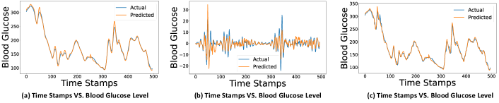
Fig. 5 highlights a demonstration of forecasting the blood glucose model with minutes for low-frequency, high-frequency, and blood glucose levels for a participant of the Ohio dataset. In Fig. 5, we can observe that the GlucoNet model forecasts the blood glucose levels accurately when PH is minutes.
We evaluate GlucoNet with three types of forecasting horizons - short (5 minutes), medium (30 minutes), and long-term (60 minutes). The average value of error metrics for different configurations of our GlucoNet compared to the baseline model is shown in Table 4. The configurations of GlucoNet that we considered are GlucoNet with or without knowledge distillation (KD) and implemented with the large transformer (teacher transformer) or the small transformer (student transformer). These configurations are GlucoNet , GlucoNet , and GlucoNet KD . Moreover, the baseline model architecture is 1D-CNN, followed by LSTM. The 1D-CNN consists of two 1D convolution layers, each with a kernel size of 3. The layers have configurations of and , respectively. The LSTM has two layers, which include and . Then, the output of LSTM is fed to three fully connected layers.
| RMSE | MAE | Square | |||||||||||||||||||||||||
| Total | 2018 | 2020 | Total | 2018 | 2020 | Total | 2018 | 2020 | |||||||||||||||||||
| PH | 5 | 30 | 60 | 5 | 30 | 60 | 5 | 30 | 60 | 5 | 30 | 60 | 5 | 30 | 60 | 5 | 30 | 60 | 5 | 30 | 60 | 5 | 30 | 60 | 5 | 30 | 60 |
| Baseline | 8.03 | 14.17 | 16.46 | 8.41 | 15.35 | 16.91 | 7.66 | 13.00 | 16.01 | 5.07 | 9.69 | 10.92 | 5.19 | 10.53 | 11.47 | 4.94 | 8.84 | 10.37 | 0.97 | 0.91 | 0.89 | 0.96 | 0.89 | 0.86 | 0.98 | 0.94 | 0.92 |
| GlucoNet | 6.31 | 9.75 | 11.68 | 7.61 | 11.32 | 13.29 | 5.00 | 8.18 | 10.07 | 3.50 | 5.12 | 7.15 | 4.17 | 5.52 | 8.00 | 2.84 | 4.73 | 6.30 | 0.98 | 0.96 | 0.94 | 0.98 | 0.94 | 0.93 | 0.99 | 0.97 | 0.96 |
| GlucoNet | 6.08 | 8.84 | 11.89 | 7.03 | 9.81 | 13.24 | 5.13 | 7.89 | 10.55 | 3.42 | 5.05 | 7.16 | 3.90 | 5.57 | 7.70 | 2.95 | 4.54 | 6.61 | 0.98 | 0.97 | 0.94 | 0.98 | 0.96 | 0.93 | 0.99 | 0.97 | 0.95 |
| GlucoNetKD | 5.89 | 8.59 | 11.77 | 6.51 | 9.30 | 12.74 | 5.28 | 7.88 | 10.80 | 3.34 | 4.97 | 7.06 | 3.79 | 5.28 | 7.45 | 2.89 | 4.65 | 6.67 | 0.99 | 0.97 | 0.95 | 0.98 | 0.97 | 0.94 | 0.99 | 0.97 | 0.95 |
Table 4 shows that GlucoNet deployed with knowledge distillation achieves efficient models without compromising performance metrics compared to GlucoNet without KD and implemented with the large Transformer.
Moreover, The average values of RMSE, MAE, and Square for different PHs (5 minutes, 30 minutes, 60 minutes) and configurations of our GlucoNet are shown in Fig. 6. In this figure, different configurations are considered different LSTMs with different numbers of memory cells or units. The configurations that are considered for comparison are GlucoNet KD , }, GlucoNet KD ,GlucoNet KD , and GlucoNet KD .
By noting Fig. 6, we can conclude that the accuracy of the model optimized for configurations of GlucoNet KD is evident. It is noteworthy that increasing the size or number of layers in the LSTM may lead to overfitting, which results in a decrease in the model’s accuracy.
Furthermore, we compared Gluconet with state-of-the-art models. Table 3 presents a comparison of GlucoNet with other state-of-the-art papers in terms of RMSE, MAE, and Square for PHs of 30 minutes and 60 minutes. The configuration of GlucoNet for this comparison is defined as GlucoNet KD . In this table, the error metrics values are reported as average for comparison. This table highlights the performance of our proposed forecasting model.
The state-of-the-art models that we compared in Table 3 included deep learning models such as long short-term memory (LSTM), 1D CNN-LSTM (GlySim), deep residual network, recurrent self-attention, and convolutional recurrent neural networks (CNN-RNN). we can note that when minutes, GlucoNet with KD achieved the lowest RMSE of and MAE of . This outperformed the next best model, MTL-LSTM, which had an RMSE of and MAE of . Also, when minutes, it achieved an RMSE of and MAE of , which is better than the GlySim, which had RMSE of and MAE of . Therefore, the GlucoNet showed significant improvements compared with another model, about and in terms of RMSE and MAE when minutes. Furthermore, when minutes GlucoNet improvements for RMSE is about and MAE is about . These results highlight the effectiveness of the proposed GlucoNet in capturing complex blood glucose dynamics and forecasting for longer-term predictions. Furthermore, the computational efficiency of the GlucoNet model compared to other models will discussed in the following section.
4.3. Accuracy-Efficiency Trade-offs
We have also compared our GlucoNet with other State-of-the-Art forecasting models in terms of accuracy-efficiency. We computed accuracy metrics, e.g., RMSE and MAE. Furthermore, the efficiency metric is computed by the total number of model parameters. Fig. 7 shows the accuracy-efficiency trade-offs of GlucoNet compared with state-of-the-art models.

We can note that GlucoNet configurations offer the best accuracy-efficiency trade-off compared to the other models. Our GlucoNet with KD achieves high accuracy with only about total parameters, which makes it suitable for potential edge deployment (Shuvo et al., 2022). Moreover, this model can be integrated into continuous glucose monitoring devices for real-time decision support.
5. Conclusion
In this paper, we presented a novel model for blood glucose level forecasting that achieves improved accuracy while maintaining computational efficiency. The GlucoNet model combines blood glucose data with event-based variables such as carbohydrate intake and insulin dosage. These event-based variables are transformed into time series features by a mathematical model. Furthermore, To address the non-linear and non-stationary nature of blood glucose time series data, Variational Mode Decomposition (VMD) is employed to decompose the data into low and high-fluctuation signal modes. The time series features of carbohydrate intake and insulin dosage are combined with low and high-fluctuation signal modes and create low-frequency features and high-frequency features. Low-frequency and high-frequency features are then fed to the LSTM and transformer models to forecast the BGL, respectively. To enhance efficiency, a knowledge distillation technique is implemented to compress the Transformer model. GlucoNet improved the RMSE by approximately while decreasing the total model parameters by compared with existing models for forecasting blood glucose. Moreover, GlucoNet shows substantial enhancements in both RMSE and MAE metrics, with improvements of about and , respectively, compared to state-of-the-art methods on participants. These results highlight GlucoNet’s potential as a more accurate and efficient tool for blood glucose forecasting.
References
- (1)
- Arefeen and Ghasemzadeh (2023) Asiful Arefeen and Hassan Ghasemzadeh. 2023. Glysim: Modeling and simulating glycemic response for behavioral lifestyle interventions. In 2023 IEEE EMBS International Conference on Biomedical and Health Informatics (BHI). IEEE, 1–5.
- Armandpour et al. (2021) Mohammadreza Armandpour, Brian Kidd, Yu Du, and Jianhua Z Huang. 2021. Deep personalized glucose level forecasting using attention-based recurrent neural networks. In 2021 International Joint Conference on Neural Networks (IJCNN). IEEE, 1–8.
- Azghan et al. (2023) Reza Rahimi Azghan, Nicholas C. Glodosky, Ramesh Kumar Sah, Carrie Cuttler, Ryan McLaughlin, Michael J. Cleveland, and Hassan Ghasemzadeh. 2023. Personalized Modeling and Detection of Moments of Cannabis Use in Free-Living Environments. In 2023 IEEE 19th International Conference on Body Sensor Networks (BSN). 1–4. https://doi.org/10.1109/BSN58485.2023.10331481
- Boiroux et al. (2010) Dimitri Boiroux, Daniel A Finan, John Bagterp Jørgensen, Niels Kjølstad Poulsen, and Henrik Madsen. 2010. Optimal insulin administration for people with type 1 diabetes. IFAC Proceedings Volumes 43, 5 (2010), 248–253.
- Chen et al. (2024) Shisen Chen, Fen Qin, Xuesheng Ma, Jie Wei, Yuan-Ting Zhang, Yuan Zhang, and Emil Jovanov. 2024. Multi-view cross-fusion transformer based on kinetic features for non-invasive blood glucose measurement using PPG signal. IEEE Journal of Biomedical and Health Informatics (2024).
- Cui et al. (2021) Ran Cui, Chirath Hettiarachchi, Christopher J Nolan, Elena Daskalaki, and Hanna Suominen. 2021. Personalised short-term glucose prediction via recurrent self-attention network. In 2021 IEEE 34th International Symposium on Computer-Based Medical Systems (CBMS). IEEE, 154–159.
- Daniels et al. (2021) John Daniels, Pau Herrero, and Pantelis Georgiou. 2021. A multitask learning approach to personalized blood glucose prediction. IEEE Journal of Biomedical and Health Informatics 26, 1 (2021), 436–445.
- Dragomiretskiy and Zosso (2013) Konstantin Dragomiretskiy and Dominique Zosso. 2013. Variational mode decomposition. IEEE transactions on signal processing 62, 3 (2013), 531–544.
- Dragomiretskiy and Zosso (2014) Konstantin Dragomiretskiy and Dominique Zosso. 2014. Variational Mode Decomposition. IEEE Transactions on Signal Processing 62, 3 (2014), 531–544. https://doi.org/10.1109/TSP.2013.2288675
- Freiburghaus et al. (2020) Jonas Freiburghaus, Aïcha Rizzotti, and Fabrizio Albertetti. 2020. A deep learning approach for blood glucose prediction of type 1 diabetes. In Proceedings of the Proceedings of the 5th International Workshop on Knowledge Discovery in Healthcare Data co-located with 24th European Conference on Artificial Intelligence (ECAI 2020), 29-30 August 2020, Santiago de Compostela, Spain, Vol. 2675. 29-30 August 2020.
- Georga et al. (2015) Eleni I Georga, Vasilios C Protopappas, Demosthenes Polyzos, and Dimitrios I Fotiadis. 2015. Evaluation of short-term predictors of glucose concentration in type 1 diabetes combining feature ranking with regression models. Medical & biological engineering & computing 53 (2015), 1305–1318.
- Hameed and Kleinberg (2020) Hadia Hameed and Samantha Kleinberg. 2020. Investigating potentials and pitfalls of knowledge distillation across datasets for blood glucose forecasting. In Proceedings of the 5th Annual Workshop on Knowledge Discovery in Healthcare Data.
- Hinton (2015) Geoffrey Hinton. 2015. Distilling the Knowledge in a Neural Network. arXiv preprint arXiv:1503.02531 (2015).
- Hochreiter (1997) S Hochreiter. 1997. Long Short-term Memory. Neural Computation MIT-Press (1997).
- Jaloli and Cescon (2023) Mehrad Jaloli and Marzia Cescon. 2023. Long-term prediction of blood glucose levels in type 1 diabetes using a cnn-lstm-based deep neural network. Journal of diabetes science and technology 17, 6 (2023), 1590–1601.
- Kargar-Barzi et al. (2024) Amin Kargar-Barzi, Ebrahim Farahmand, Nooshin Taheri Chatrudi, Ali Mahani, and Muhammad Shafique. 2024. An Edge-Based WiFi Fingerprinting Indoor Localization Using Convolutional Neural Network and Convolutional Auto-Encoder. IEEE Access 12 (2024), 85050–85060. https://doi.org/10.1109/ACCESS.2024.3412676
- Kaur et al. (2021) Chamandeep Kaur, Amandeep Bisht, Preeti Singh, and Garima Joshi. 2021. EEG Signal denoising using hybrid approach of Variational Mode Decomposition and wavelets for depression. Biomedical Signal Processing and Control 65 (2021), 102337.
- Khadem et al. (2023) Heydar Khadem, Hoda Nemat, Jackie Elliott, and Mohammed Benaissa. 2023. Blood glucose level time series forecasting: nested deep ensemble learning lag fusion. Bioengineering 10, 4 (2023), 487.
- Kraegen et al. (1981) EW Kraegen, DJ Chisholm, and Mary E McNamara. 1981. Timing of insulin delivery with meals. Hormone and Metabolic Research 13, 07 (1981), 365–367.
- Lee et al. (2024) Jung Min Lee, Rodica Pop-Busui, Joyce M Lee, Jesper Fleischer, and Jenna Wiens. 2024. Shortcomings in the Evaluation of Blood Glucose Forecasting. IEEE Transactions on Biomedical Engineering (2024).
- Lee et al. (2023) Sang-Min Lee, Dae-Yeon Kim, and Jiyoung Woo. 2023. Glucose transformer: Forecasting glucose level and events of hyperglycemia and hypoglycemia. IEEE Journal of Biomedical and Health Informatics 27, 3 (2023), 1600–1611.
- Li et al. (2019a) Kezhi Li, John Daniels, Chengyuan Liu, Pau Herrero, and Pantelis Georgiou. 2019a. Convolutional recurrent neural networks for glucose prediction. IEEE journal of biomedical and health informatics 24, 2 (2019), 603–613.
- Li et al. (2019b) Kezhi Li, Chengyuan Liu, Taiyu Zhu, Pau Herrero, and Pantelis Georgiou. 2019b. GluNet: A deep learning framework for accurate glucose forecasting. IEEE journal of biomedical and health informatics 24, 2 (2019), 414–423.
- Liu et al. (2022) Wei Liu, Y. Liu, Shuang Li, and Yang Chen. 2022. A Review of Variational Mode Decomposition in Seismic Data Analysis. Surveys in Geophysics 44 (2022), 323–355. https://api.semanticscholar.org/CorpusID:253502339
- Mamun et al. (2022a) Abdullah Mamun, Krista S Leonard, Matthew P Buman, and Hassan Ghasemzadeh. 2022a. Multimodal Time-Series Activity Forecasting for Adaptive Lifestyle Intervention Design. In 2022 IEEE-EMBS International Conference on Wearable and Implantable Body Sensor Networks (BSN). IEEE, 1–4.
- Mamun et al. (2022b) Abdullah Mamun, Seyed Iman Mirzadeh, and Hassan Ghasemzadeh. 2022b. Designing Deep Neural Networks Robust to Sensor Failure in Mobile Health Environments. In 2022 44th Annual International Conference of the IEEE Engineering in Medicine & Biology Society (EMBC). IEEE, 2442–2446.
- Marling and Bunescu (2020) Cindy Marling and Razvan Bunescu. 2020. The OhioT1DM dataset for blood glucose level prediction: Update 2020. In CEUR workshop proceedings, Vol. 2675. NIH Public Access, 71.
- Martinsson et al. (2020) John Martinsson, Alexander Schliep, Björn Eliasson, and Olof Mogren. 2020. Blood glucose prediction with variance estimation using recurrent neural networks. Journal of Healthcare Informatics Research 4 (2020), 1–18.
- Rabby et al. (2021) Md Fazle Rabby, Yazhou Tu, Md Imran Hossen, Insup Lee, Anthony S Maida, and Xiali Hei. 2021. Stacked LSTM based deep recurrent neural network with kalman smoothing for blood glucose prediction. BMC Medical Informatics and Decision Making 21 (2021), 1–15.
- Rubin-Falcone et al. (2020) Harry Rubin-Falcone, Ian Fox, and Jenna Wiens. 2020. Deep Residual Time-Series Forecasting: Application to Blood Glucose Prediction. KDH@ ECAI 20 (2020), 105–109.
- Shanthi (2011) S Shanthi. 2011. A novel approach for the prediction of glucose concentration in type 1 diabetes ahead in time through ARIMA and differential evolution. Adv. Eng. Inform. 38 (2011), 4182–4186.
- Shuvo and Islam (2023) Md Maruf Hossain Shuvo and Syed Kamrul Islam. 2023. Deep multitask learning by stacked long short-term memory for predicting personalized blood glucose concentration. IEEE Journal of Biomedical and Health Informatics 27, 3 (2023), 1612–1623.
- Shuvo et al. (2022) Md Maruf Hossain Shuvo, Syed Kamrul Islam, Jianlin Cheng, and Bashir I Morshed. 2022. Efficient acceleration of deep learning inference on resource-constrained edge devices: A review. Proc. IEEE 111, 1 (2022), 42–91.
- Syafrudin et al. (2022) Muhammad Syafrudin, Ganjar Alfian, Norma Latif Fitriyani, Imam Fahrurrozi, Muhammad Anshari, and Jongtae Rhee. 2022. A Personalized Blood Glucose Prediction Model Using Random Forest Regression. In 2022 ASU International Conference in Emerging Technologies for Sustainability and Intelligent Systems (ICETSIS). IEEE, 295–299.
- ur Rehman and Aftab (2019) Naveed ur Rehman and Hania Aftab. 2019. Multivariate variational mode decomposition. IEEE Transactions on signal processing 67, 23 (2019), 6039–6052.
- van Doorn et al. (2021) William PTM van Doorn, Yuri D Foreman, Nicolaas C Schaper, Hans HCM Savelberg, Annemarie Koster, Carla JH van der Kallen, Anke Wesselius, Miranda T Schram, Ronald MA Henry, Pieter C Dagnelie, et al. 2021. Machine learning-based glucose prediction with use of continuous glucose and physical activity monitoring data: The Maastricht Study. PloS one 16, 6 (2021), e0253125.
- Vaswani (2017) A Vaswani. 2017. Attention is all you need. Advances in Neural Information Processing Systems (2017).
- Wang et al. (2020) Wenbo Wang, Meng Tong, and Min Yu. 2020. Blood glucose prediction with VMD and LSTM optimized by improved particle swarm optimization. IEEE Access 8 (2020), 217908–217916.
- Wenbo et al. (2021) Wang Wenbo, Shen Yang, and Chen Guici. 2021. Blood glucose concentration prediction based on VMD-KELM-AdaBoost. Medical & Biological Engineering & Computing 59 (2021), 2219–2235.
- Xue et al. (2024) Yuewei Xue, Shaopeng Guan, and Wanhai Jia. 2024. BGformer: An improved Informer model to enhance blood glucose prediction. Journal of Biomedical Informatics 157 (2024), 104715.
- Yousefi et al. (2023) Mojtaba Yousefi, Jinghao Wang, Øivind Fandrem Høivik, Jayaprakash Rajasekharan, August Hubert Wierling, Hossein Farahmand, and Reza Arghandeh. 2023. Short-term inflow forecasting in a dam-regulated river in Southwest Norway using causal variational mode decomposition. Scientific Reports 13, 1 (2023), 7016.
- Zhang et al. (2019) Linfeng Zhang, Jiebo Song, Anni Gao, Jingwei Chen, Chenglong Bao, and Kaisheng Ma. 2019. Be your own teacher: Improve the performance of convolutional neural networks via self distillation. In Proceedings of the IEEE/CVF international conference on computer vision. 3713–3722.