Hunter: Using Change Point Detection to Hunt for Performance Regressions
Abstract.
Change point detection has recently gained popularity as a method of detecting performance changes in software due to its ability to cope with noisy data. In this paper we present Hunter, an open source tool that automatically detects performance regressions and improvements in time-series data. Hunter uses a modified E-divisive means algorithm to identify statistically significant changes in normally-distributed performance metrics. We describe the changes we made to the E-divisive means algorithm along with their motivation. The main change we adopted was to replace the significance test using randomized permutations with a Student’s t-test, as we discovered that the randomized approach did not produce deterministic results, at least not with a reasonable number of iterations. In addition we’ve made tweaks that allow us to find change points the original algorithm would not, such as two nearby changes. For evaluation, we developed a method to generate real timeseries, but with artificially injected changes in latency. We used these data sets to compare Hunter against two other well known algorithms, PELT and DYNP. Finally, we conclude with lessons we’ve learned supporting Hunter across teams with individual responsibility for the performance of their project.
1. Introduction
Testing the performance of distributed databases, such as Apache Casandra, is an integral part of the development process and is often incorporated into Continuous Integration pipelines where performance tests and benchmarks can be run periodically or in response to pushing changes to source code repositories. But given the complex nature of distributed systems, their performance is often unstable and performance test results can fluctuate from run to run even on the same hardware. This result instability is due to a number of factors including variability of the underlying hardware (Duplyakin et al., 2020), background processes and CPU frequency scaling at the OS level, and application-level request scheduling and prioritisation (TAL, 2014). All of this makes the job of identifying whether the change in performance is the result of a software change or simply noise from the test extremely difficult to do automatically. Threshold-based techniques are covered in the literature, but these methods do not handle noise in benchmark data well and require that threshold values be set per-test (Daly et al., 2020). Additionally, thresholds need to be periodically tuned as performance improvements are added and new baselines are established.
In the past, we have relied heavily on experienced engineers to visually inspect graphs and benchmark data to identify changes in performance. However, this suffers from a number of drawbacks including:
-
•
Expert knowledge for identifying changes is difficult to teach other engineers
-
•
Small teams of experts have a limit on the number of tests they can inspect
-
•
Even experienced engineers can miss changes
Because of these drawbacks, we have recently created Hunter(Piotr Kołaczkowski, [n.d.]), an open source tool that uses change point detection to find statistically significant changes in time-series data. Change point detection has recently gained favour as a method of coping with the inherent instability, or noise, in performance test and benchmark data (Daly et al., 2020) and can identify both performance regressions and improvements.
Hunter was designed with the goal of eliminating the need for a dedicated group of engineers to sift through performance test results. Instead, individual teams can feed their benchmark data to a central datastore which Hunter pulls from and analyses. We use Hunter for validating multiple releases across various distributed database and streaming products which has required that we make Hunter intuitive and user-friendly for engineers that are experts in their particular area but not performance experts.
The contributions in this paper are:
-
•
We present an open-source tool that can run change point detection on any time-series data containing multiple metrics in either a .CSV file or stored on a graphite server.
-
•
We discuss the modifications we have made to the E-divisive means algorithm to improve its performance and predictability of results.
-
•
We develop a method for generating timeseries of real benchmarking results, with artificially injected changes to latency at discrete points in time. This allows us to evaluate the accuracy of an algorithm objectively, against a known set of correct change points.
-
•
We compare Hunter (modified E-divisive means) against two other change point detection algorithms, DYNP and PELT.
-
•
We share the lessons that we have learned from running Hunter in a multi-team environment where each team is responsible for a different product and favors different benchmarks.
2. High-Level Overview
Hunter is a command-line tool, written in Python, that detects statistically significant changes in time-series data stored either in a CSV file or on a graphite server. It is designed to be easily integrated into build pipelines (Grambow et al., 2019) and provide automated performance analysis that can decide whether code should be deployed to production. As well as printing change point data on the command-line, Hunter also includes support for Slack and can be configured to send results to a Slack channel.
2.1. Data Source
Hunter can run analysis on data pulled from a graphite server or from data contained in an CSV file. Graphite support was necessary to integrate Hunter into our testing and deployment workflow. If developers are not using graphite as their central repository of benchmark data, the CSV support provides a common denominator for feeding data to Hunter.
2.2. Configuration
The data sources that Hunter uses are specified in a YAML configuration file. This configuration file has sections for graphite servers, Slack tokens, and data definitions. Hunter even supports templating which allows common definitions to be reused and avoids test definition duplication. Since we routinely use Hunter on hundreds of tests and metrics, the template feature helps to keep our configuration file small. For example, we use graphite metric prefixes to group related metrics together so that all metrics for a specific Apache Cassandra version are linked by a common string.
One example of this is the test db.20k-rw-ts.fixed, a benchmark running on Datastax Enterprise that performs read and write operations at a fixed rate of throughput. We run this test in both a configuration with replication factor 1 and with replication factor 3 and yet despite this difference we can reuse around 95% of the Hunter configuration because the metric types are the same.
Below is an example configuration file.
graphite:
  url: http://graphite.local
  suffixes:
    - ebdse_read.result

templates:
  common_metrics:
    metrics:
      throughput:
        scale: 1
        direction: 1
      p99:
        scale: 1.0e-6
        direction: -1

tests:
  db.20k-rw-ts.fixed:
    inherit:
    - common_metrics
    tags:
    - db.20k-rw-ts.fixed.1-bm2small-rf-1
    prefix: performance_regressions.db.20k-rw-ts.fixed
For test data in CSV files, Hunter allows users to specify attributes of the file such as file path, which columns contain timestamps, which contains metrics, and the delimiter character used to separate fields on each line.
2.3. Continuous Integration
Since Hunter is a simple Python application, it has proven trivial to connect with different teams’ CI pipelines. We use a docker image to run Hunter against daily performance test results which are stored on a central graphite server. The Docker image is launched from a Jenkins job that runs once a day.
2.4. Sending Results to Slack
After running change point detection on a given time-series, Hunter can submit the results of its analysis to a Slack channel. We have found that this is the perfect location to notify developers of changes in performance mainly because each channel is already categorised by team or project. Developers usually triage the results of Hunter by investigating any unexpected changes in performance to identify whether there is a genuine change in performance for the product or the result was caused by noise in the workload or the platform.
Having Hunter’s results displayed in such a prominent location as Slack channels has resulted in improvements to the underlying infrastructure used to run performance tests. When test results show frequent fluctuations because of noise from the platform, one of our teams improved the stability of those platforms so that they are provided with more actionable results from Hunter.
3. Implementation
Hunter is built on top of the E-divisive Means algorithm available in the signal_processing_algorithms library from MongoDB (MongoDB, [n.d.]b) but we have extended it in two ways to improve its efficiency (so that we can generate results faster) and to get repeatable results when performing multiple iterations on the same data set.
3.1. E-divisive Means Algorithm
The E-divisive means (Matteson and James, 2014) is an offline change point detection algorithm that uses hierarchical estimation to estimate the number and locations of change points in a distribution. Since it’s a nonparametric method, it makes no assumptions about the underlying data distribution or the change in distribution and is well suited for use with benchmarking data that is often non-normal. The hierarchical aspect comes into play when deciding which collection of data points to search for change points. E-divisive means divides the time-series into two parts and recursively searches for change points.
Individual points are tested using a test statistic from previous change points which the literature calls q̂, and the p-value of q̂ is determined using random permutation testing which requires multiple calculations. Using random permutations comes with a performance cost and we found that detecting change points took an unreasonably long time for our data set. Additionally, because the permutations are random we found that the results of Hunter were non-deterministic and varied from run to run. It is possible to reduce the non-determinism in the results by increasing the number of permutations but this has the negative effect of increasing Hunter’s runtime. In our case running Hunter using the standard E-divisive means algorithm on hundreds of data points for a single test and single metric took 2-3 seconds. But to validate a nightly build or release, developers need the ability to run change point detection on tens of tests where each test recorded tens of metrics. This would push the runtime to several minutes, which was no longer ideal.
3.2. Significance Testing
When initially developing Hunter we profiled the code to understand which parts were taking the longest to detect change points in our data. We discovered that the vast majority of the time was spent performing significance testing. This wasn’t entirely surprising given the use of the q̂ statistic and its reliance on random permutations. We switched to using Student’s t-test and saw the runtime of Hunter reduce by an order of magnitude as well as providing consistent results when run multiple times on the same data set. While Student’s t-test is not a robust measure of statistical significance for arbitrary data sets, it turned out it works extremely well for our scenario.
We also tested using the Mann-Whitney U test. This would have been appealing since, unlike the Student’s t-test, it is a non-parametric test that doesn’t assume the input data is normally distributed. But it turned out to not behave very well on small amounts of data, as it requires 30 points to be conclusive. In contrast both the original E-Divisive, and our Student’s t-version, are able to find changes in extremely short time series with only 4-7 points. Since E-Divisive is a hierarchical algorithm that splits the original time series into ever smaller windows, this is a significant difference.
3.3. Fixed-Sized Windows
As we began using Hunter on larger and larger data series, we discovered that change points identified in previous runs would suddenly disappear from Hunter’s results. This issue turned out to be caused by performance regressions that were fixed shortly after being introduced. This is a known issue with E-divisive means and is discussed in (Daly et al., 2020). Because E-divisive means divides the time series into two parts, most of the data points on either side of the split showed similar values. The algorithm therefore, by design, would treat the two nearby changes as a temporary anomaly, rather than a persistent change, and therefore filter it out.
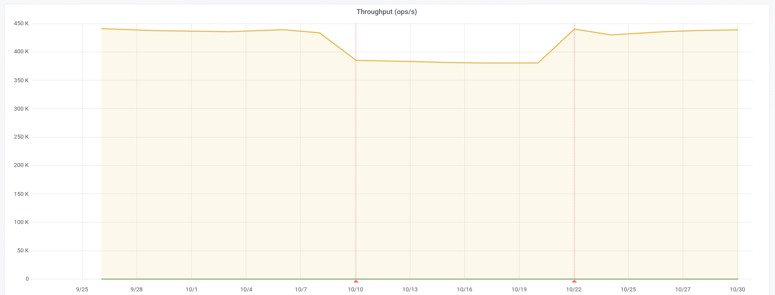
Figure 1 illustrates this issue.
Our solution to this problem was to split the entire time series into fixed-sized windows and run the E-divisive means algorithm on each window individually. Change points that exist at window boundaries require special attention since change point detection algorithms in general are unable to identify whether the most recent point in a data series is a change point. To address this problem Hunter allows the windows to overlap and care is taken so that a change point isn’t reported multiple times because it exists in multiple windows.
3.4. Weak Change Points
Splitting the data series into windows partially addresses the problem of missing change points in large data sets, but we also needed a method of forcing the E-divisive means algorithm to continue recursively analysing the data series. The E-divisive means algorithm terminates when the significance test, Student’s t-test in Hunter, fails. If the algorithm first selects a change point with a p-value above the threshold set by the user (usually 0.05), it will terminate immediately, even if it would have detected change points below the p-value had it continued. We refer to change points that fail the significance test but would lead to other points below the p-value as weak change points.
The process of handling weak change points has two steps. First, we use a larger p-value threshold when splitting so that it allows detection of weak change points. Second, we reevaluate the p-values and merge the split data series in a bottom-up way by removing change points that have a p-value above the smaller, user-specified threshold. We found that without forcing recursion to continue Hunter would miss some change points. Our modification results in much more accurate p-values.
Additionally, we filter out change points that show a small relative change, e.g. change points where the difference in metric value is below 5%. This relative threshold acts as a filter to discard change points that are not actionable, i.e. change points that are too small for developers to reproduce or verify a fix.
4. Evaluation
We evaluated our algorithms using benchmark data taken from a daily Gatling (Gatling, [n.d.]) performance test on Datastax Enterprise. The benchmark data was saved to a CSV file and passed to Hunter using the following command-line:
poetry run hunter analyse db-gatling.csv
.
The data in db-gatling.csv contains 175 entries and covers 15 months’ worth of data. There are multiple performance changes contained within, both improvements (higher throughput or lower latency) and regressions (lower throughput or higher latency).
| Algorithm | Mean Duration | Mean 95% CI | Change points | Change points stddev |
|---|---|---|---|---|
| Permutation | 2.221 | 2.209, 2.233 | 16 | 1.174 |
| Student’s t-test | 1.863 | 1.853, 1.873 | 20 | 0 |
| Student’s + Weak Change Points | 1.594 | 1.584, 1.603 | 16 | 0 |
We opted for reading the data from a CSV file to avoid network communication delays with the graphite server influencing the duration of each run. Every algorithm was run 30 times on the same CSV file and the mean value, along with 95% confidence intervals, are reported in Table 1.
Since we found that the permutation algorithm produced unstable results, we have also included the average number of change points detected for each of the algorithms in Table 1 as well as the standard deviations.
4.1. Quickly Reverted Regressions
Around 2020-10-10 on the graph in Figure 1 we can see a drop in the throughput. This performance regression was caused by a change to the way network packet decoding and processing was done in Datastax Enterprise. This problematic change was reverted on 2020-10-21 which explains why the throughput metric returns to previous values shortly after. Two red lines demarcate the data range where the regression is present. This is a known problem with change point detection and is explicitly mentioned in (Daly et al., 2020).
Both the Student’s t-test and weak change points algorithms detected this regression and revert in each of the 30 runs through the data. The permutation based algorithm, only detected these changes for 15 of the 30 runs, or 50% of the time.
4.2. MongoDB Performance Test Result Dataset
We also used the publicly available MongoDB Performance Test Result Dataset (MongoDB, [n.d.]a) to compare the performance of E-divisive means with random permutations, and Student’s t-test with weak change points filtering as the statistical significance test. This is the same data set used in (Daly et al., 2020), so this analysis should be comparable and familiar to the emerging change point detection community.
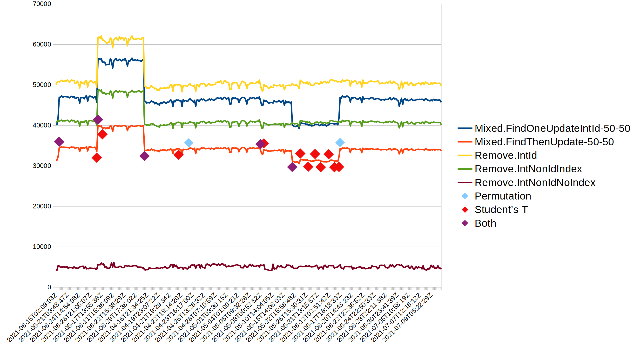
We arbitrarily selected 5 tests from the microbenchmark suite, and only focus on the max_ops_per_sec result. All results are from task misc_read_commands and variant linux-wt-standalone. The 5 timeseries are shown in Figure 2. To avoid clutter, only one timeseries was decorated with the change points found, but the results for the other 4 are similar.
As discussed above, the original E-divisive algorithm is not deterministic. Table 2 shows how many change points were found for 100 iterations of each timeseries. The results are alarming. For example for Remove.IntNonIdNoIndex (row 5) it finds 4 change points 43% of the time, 3 points 50% of the time, but 7% of the time it finds zero change points!
Figure 2 also shows the other main issue that we have addressed. When a regresion is quickly followed by a fix or rebound, then the original algorithm tends to ignore one or both changes as noise. The 9th change point in the graph is such an example, it is only found due to the approach with fixed sized windows in this work.
Finally we can clearly see that our implementation finds many more change points. (The red diamonds are found only with the Student’s t-test configuration.) This is an expected result as most of the modifications are motivated by making the algorithm as sensitive as possible. Whether all 16 change points are meaningful is ultimately a subjective judgement, but looking closely at the graph one can at least understand why the algorithm would have chosen each point. The implementation offers to filter out changes that are too small to be actionable, but this feature was not used in these tests, as we wanted to show the full output of our modified E-divisive algorithm, without post filtering.
An obvious question we can already anticipate is that if the original implementation from MongoDB performs thís poorly, how come MongoDB itself has used it so successfully? The answer is that a a higher level in MongoDB’s performance CI was designed such that if a point was once flagged as a change point, the system will forever remember it. This way change points would not randomly disappear while a developer is already working to fix it, and likewise a point marked as a false positive will remain muted and not re-appear the next day. But the effect relative to the problems highlighted in this paper is that the overall MongoDB CI system will eventually find and remember all change points, even if on a given day the E-divisive algorithm may stop early and only return a subset. This higher level system was documented in (Ingo and Daly, 2020) and the recorded change points are also part of (MongoDB, [n.d.]a).
| Algorithm | Test name | 0 | 1 | 2 | 3 | 4 | 5 | 6 | 7 | 8 | 9 | 12 | 14 | 16 | 18 |
|---|---|---|---|---|---|---|---|---|---|---|---|---|---|---|---|
| Permutation | Mixed.FindOneUpdateIntId-50-50 | 1 | 1 | 98 | |||||||||||
| Permutation | Mixed.FindThenUpdate-50-50 | 1 | 99 | ||||||||||||
| Permutation | Remove.IntId | 64 | 32 | 4 | |||||||||||
| Permutation | Remove.IntNonIdIndex | 61 | 34 | 5 | |||||||||||
| Permutation | Remove.IntNonIdNoIndex | 7 | 50 | 43 | |||||||||||
| Student’s + Weak | Mixed.FindOneUpdateIntId-50-50 | 100 | |||||||||||||
| Student’s + Weak | Mixed.FindThenUpdate-50-50 | 100 | |||||||||||||
| Student’s + Weak | Remove.IntId | 100 | |||||||||||||
| Student’s + Weak | Remove.IntNonIdIndex | 100 | |||||||||||||
| Student’s + Weak | Remove.IntNonIdNoIndex | 100 |
4.3. Evaluation with a Dataset with Known Change Points
One weakness in the above analysis, and to our knowledge all previous literature published on this topic so far, is that judging the accuracy of the algorithm or its implementation is always subjective. Ultimately it’s the human evaluator who decides whether a reported change point is a true positive, or ”useful”, or ”actionable”. And note that those may not be the same! This is because an objective truth about the correct set of change points is not available. If we had that knowledge, we would not have needed this system to begin with.
It’s of course possible to generate synthetic timeseries with changes injected at known steps, such as a sine wave or even white noise, where the mean or amplitude is changing at discrete points. However these tests tend to feel naive and E-divisive performs quite well against them.
To obtain a real data set, we employed Chaos Mesh(Cloud Native Computing Foundation, [n.d.]) to artificially generate network latency in the system under test. In other words we artificially injected real changes, at known points in time, into a real benchmark producing otherwise realistic results. The benchmark used was to test Cassandra with the same toolchain used for CI(Datastax, [n.d.]).
In order to create different time series, we decided on a group of variables that we varied to generate varying scenarios. We created 9 different scenarios by altering the values of the following variables: number of changepoints, magnitude of change of variance between groups, magnitude of change between groups and the length of groups. A group is defined as the set of points occurring between two changepoints. Each scenario contains 5 test series, each with a minor variation. The scenarios themselves can be grouped into three categories. The first scenario, change in mean, creates change points by changing the mean of the groups. The variance remains relative constant. Similarly, change in variance has constant mean and varying variance. This case is great to replicate noisy environment’s. Change in both mean and variance realistically replicates noisy environment’s with random latencies.
Note that the timeseries used for this evaluation is different from those in previous sections. Whereas previous timeseries have been a sequence of (nightly) builds, and the data points represent values like average throughput during a test, in this evaluation the timeseries is from a single benchmark, and the values are snapshots each second. This is because waiting for a year to create a time series of true nightly builds was not practical.
4.3.1. Evaluation Metrics
Having obtained data sets with known change points, we can now employ objective statistical tests to measure the accuracy of Hunter. Essentially we have recast the evaluation task as a machine learning problem, where an algorithm is expected to produce a known output from a given input training dataset.
We will evaluate hunter using two metrics, F1 score and Rand Index. In particular we will be evaluating the p99 metric. p99 indicates that 1 in every 100 users will encounter latency. It is a common industry standard and also used for performance targets when developing Cassandra.
4.3.2. True Positives
We will be using the following two variables to represent the sets of ground truth and predicted points:
True positives are defined as the set of change-points in the detected class that are real change points i.e they are present in the set. M represents the scope of error. If the difference between the predicted points and the true changepoint in less that or equal to M we will consider it as a correcty predicted changepoint.
It was important to ensure that there were no duplication’s ie. if two points in the predicted set were in the margin of error of the same point in . A changepoint in was marked as visited once a point in was within and added to set and can not be considered again.
4.3.3. F1 Score
The reasons for using the F1 Score to calculate the accuracy of hunter are that it is unaffected by the size and the density of data, it penalizes false positives and credits correct detections.
F1 score is defined as
Precision is the proportion of predicted change points that are true change points:(Truong et al., 2019)
Recall is the proportion of true change points that are well predicted:(Truong et al., 2019)
4.3.4. Rand Index
Another metric we evaluated on was the rand index.
-
•
TP : correctly predicts the positive class : True change points calculated
-
•
TN : correctly predicts the negative class : None in this case
-
•
FP : model incorrectly predicts positive class :
-
•
FN :model incorrectly predicts negative class:
4.3.5. Benchmarking against PELT and DYNP
With an objective truth to benchmark against, it also becomes possible to compare Hunter against alternative change point detection algorithms. We therefore also present results from two other well-known offline algorithms PELT and DYNP. These algorithms were used using the ruptures package in python.(Truong et al., 2019)
4.3.6. Results
We ran hunter over 45 test runs. The test runs were ran on a GKE cluster using Kubernetes. The cluster was ran on 4 x n2-standard-4 nodes in zone us-central1-a.
All the algorithms were evaluated on two metrics. It can be seen that hunter has consistently outperformed both pelt and dynp on both the metrics. In all the experiments we had an margin of error as 10 seconds.
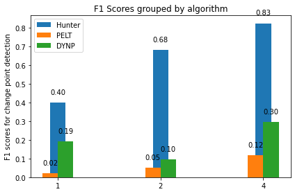
4.3.7. Correlation to the number of points
There is a positive correlation between the number of points and accuracy. As the number of points increase so does hunter’s performance. For Figure 3 it can be seen that hunter outperformed both PELT and DYNP with a huge margine.
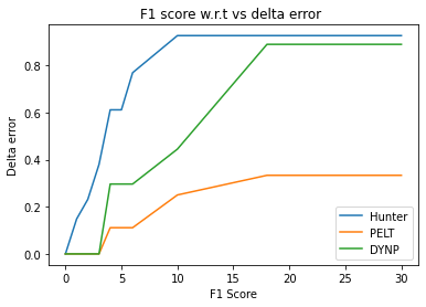
4.3.8. Correlation between delta error and algorithms
Hunter’s performance increases if we allow a larger margin of error. Hunter is able to get an F1 score of 0.1481 with an delta error of one second, where PELT and DYNP need a margin of error of at least 3 seconds to get a non-zero score. This is a key characteristic why E-divisive has served us well for detecting regressions in CI. Preferably we like to know the exact commit that caused a regression, not just the general area whereabouts a regression is suspected. E-divisive is superior in satisfying especially this requirement! The performance of all algorithms increases drastically as we give them slightly more flexibility in terms of margin of error. With a margin of error of 4 seconds we see that the performance increases to 0.612 for Hunter. DYNP starts to catch up with Hunters accuracy at 15 seconds.
| Algorithm | Hunter | Pelt | Dynp | |||
| Metric | ||||||
| Single Change Point | ||||||
| Scenario1 | 0.261904 | 0.166667 | 0.0 | 0.0 | 0.0 | 0.0 |
| Scenario2 | 0.466667 | 0.305556 | 0.027027 | 0.013698 | 0.285714 | 0.166667 |
| Scenario3 | 0.466667 | 0.305556 | 0.040556 | 0.020698 | 0.285714 | 0.166667 |
| Two Change Points | ||||||
| Scenario4 | 0.666667 | 0.666667 | 0.060606 | 0.031746 | 0.190476 | 0.111112 |
| Scenario5 | 0.888889 | 0.833334 | 0.090909 | 0.047619 | 0.095238 | 0.055556 |
| Scenario6 | 0.490476 | 0.327777 | 0.0 | 0.0 | 0.0 | 0.0 |
| Four Change Points | ||||||
| Scenario7 | 0.925926 | 0.866667 | 0.249999 | 0.142857 | 0.444445 | 0.285714 |
| Scenario8 | 0.731313 | 0.579365 | 0.085713 | 0.045073 | 0.095238 | 0.055556 |
| Scenario9 | 0.818182 | 0.714286 | 0.016460 | 0.00843 | 0.0 | 0.0 |
5. Lessons Learned
We have now been operating Hunter for multiple teams for close to 2 years. In that time we’ve made a number of improvements in addition to the algorithmic changes covered in Section 3. The lessons we have learned, and the changes made in response, helped Hunter to become the de facto choice for statistical significance detection inside of DataStax.
5.1. More Data Points Are Better
We originally started off with 2 weeks worth of data points. Given that performance tests were run once a day this gave us 14 data points. This decision was primarily because we wanted to avoid the delay in collecting lots of data from our graphite server. This proved to be far too few data points to get meaningful results from Hunter and we increased it to a month (around 30) by default. This wider time range has allowed Hunter to deal with noise in the results much better and now we see fewer false positive change points. We plan to experiment with data sets covering a longer period of time in the future to see whether we can reduce the false positive rate even further.
5.2. New Change Points Matter Most
Once a change point has been reported to a developer it does not make sense to keep reporting it. When Hunter discovers many change points, reporting them via Slack can make the results overwhelming and make it difficult for developers to analyse. Things are made worse if a change point signals a performance regression that has since been fixed because Hunter will report both the old regression and more recent improvement as separate changes.
To quieten the output of Hunter’s Slack feature, we capped results to only show change points from the last 7 days. While this does ignore valuable data because the magnitude of the change point can be updated as new data is processed, those changes are not important enough to spam everyone on the Slack channel. In the case where developers need to see the full list of results they can run Hunter manually on the data series.
5.3. Change Point Detection Cannot Fix Noisy Data
One of the teams using Hunter was afflicted with frequent change point messages via the Slack bot. After investigating these change points they discovered that the performance of the application hadn’t changed, rather the change in benchmark results was caused by unstable hardware performance in a private data center. Changes of +- 10% for the median latency were typical.
While Hunter can detect statistically significant changes in time series data, it is still not impervious to data that contains wildly fluctuating points such as that produced by running benchmarks on untuned hardware.
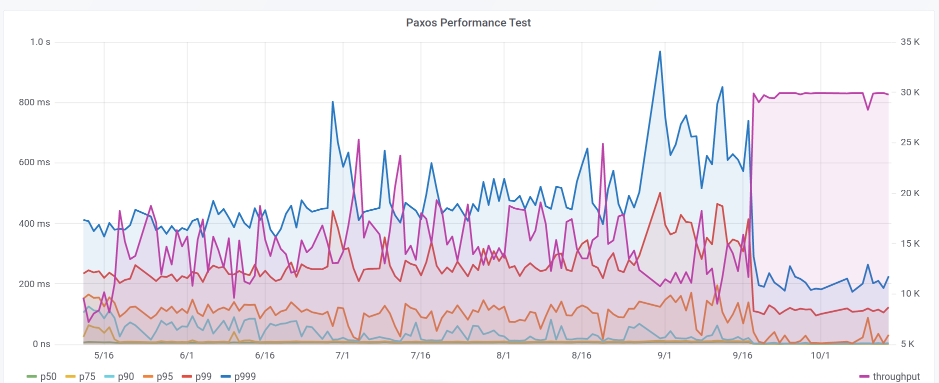
However, the fact that the team was unable to fully take advantage of Hunter motivated them to investigate the underlying issue and then migrate their benchmarks and tests to the cloud, which was shown to produce more repeatable results than the internal benchmarking lab hardware. After the migration, the benchmark results were much more stable and Hunter produced far fewer false positives. Figure 5 shows benchmark data for a single Paxos-based performance test. Before running the test on the public cloud on 2021-09-18 Hunter detected 3 change points per month, on average. All of these were false positives, that is changes in results that were not caused by software or configuration modifications. After the migration Hunter hasn’t detected a single false positive.
6. Related Work
We used the work in (Daly et al., 2020) directly when creating Hunter and the novel contributions in this paper address some of the open questions posed there. Specifically, the authors of (Daly et al., 2020) noted the bias inherent in the E-divisive means algorithm which favours detecting change points in the center of clusters. They make up for this bias by combining change point detection with anomaly detection which can identify large changes in performance as soon as the first data point in the new series is seen. Our use of windows for analysing data series addresses this same bias without resorting to anomaly detection which lacks the same sensitivity to changes as change point detection. Additionally, we are able to detect changes sooner, usually within 1-2 days.
Continuous Benchmarking (Grambow et al., 2019) is a common technique for ensuring the performance of a product is maintained or improved as new code is merged into the source code repository and the literature includes examples of using change point detection (Daly, 2021) and threshold-based methods to identify changes in software performance (Rehmann et al., 2016) as part of a continuous integration pipeline. Multiple change point detection algorithms can also be combined into an ensemble which can outperform the individual algorithms (van der Horst, 2021) when identifying performance changes.
The change point detection literature is vast and (Aminikhanghahi and Cook, 2017) and (Truong et al., 2019) provide excellent overviews and taxonomies of online and offline, supervised vs unsupervised, change point detection algorithms. In (Aminikhanghahi and Cook, 2017) in particular, online sliding window algorithms are covered in detail.
Online change point detection has also been applied to identifying changes in performance. (Zhao et al., 2020) combines change point detection with probabilistic model checking of interval Markov chains to promptly detect changes in the parameters of software systems and verify the system’s correctness, reliability, and performance.
Running performance tests in the cloud is known to be susceptible to performance variability (Uta et al., 2020) even when running the same software on the same hardware at different times. Historical performance data can be used to predict the future performance in cloud environments and (Zhao et al., 2021) explores two change point detection algorithms, robseg and breakout, to predict variability in the cloud which enables users to plan repeatable experiments. (Eismann et al., 2021) uses the E-divisive means algorithm to answer the question: does performance stability of serverless applications vary over time?
7. Conclusion
Detecting performance regressions across a range of product versions requires automation to be able to identify them quickly and without needing expert developers to manually detect them. Change point detection has emerged as a solution to this problem because of its ability to cope with noise in the data that is inherent to performance testing.
Hunter is an open source(Piotr Kołaczkowski, [n.d.]) tool that uses change point detection to automatically identify changes in time-series data, taken from either a graphite server or CSV file, and report the presence of change points. Hunter extends the E-divisive Means algorithm to incorporate a Student’s t-test which removes the indeterminism present in the original version and provides reproducible results every time it is run on a single data series. We also introduced a sliding window technique to detect change points that are temporally close to each other. In addition to outperforming the original E-divisive means implementation, Hunter seems to also outperform two other well known algorithms, PELT and DYNP.
8. Acknowledgments
We are grateful to Guy Bolton King for his contributions to Hunter.
References
- (1)
- TAL (2014) 2014. Tales of the Tail: Hardware, OS, and Application-Level Sources of Tail Latency (Seattle, WA, USA). Association for Computing Machinery, New York, NY, USA. https://doi.org/10.1145/2670979.2670988
- Aminikhanghahi and Cook (2017) Samaneh Aminikhanghahi and Diane Cook. 2017. A Survey of Methods for Time Series Change Point Detection. Knowledge and Information Systems 51 (05 2017). https://doi.org/10.1007/s10115-016-0987-z
- Cloud Native Computing Foundation ([n.d.]) Cloud Native Computing Foundation. [n.d.]. Chaos Mesh: A Powerful Chaos Engineering Platform for Kubernetes. https://chaos-mesh.org/ Accessed: 2022-10-20.
- Daly (2021) David Daly. 2021. Creating a Virtuous Cycle in Performance Testing at MongoDB. In Proceedings of the ACM/SPEC International Conference on Performance Engineering (Virtual Event, France) (ICPE ’21). Association for Computing Machinery, New York, NY, USA, 33–41. https://doi.org/10.1145/3427921.3450234
- Daly et al. (2020) David Daly, William Brown, Henrik Ingo, Jim O’Leary, and David Bradford. 2020. The Use of Change Point Detection to Identify Software Performance Regressions in a Continuous Integration System. In Proceedings of the 2020 ACM/SPEC International Conference on Performance Engineering(ICPE ’20) (2020). https://doi.org/10.1145/3358960.3375791
- Datastax ([n.d.]) Datastax. [n.d.]. Fallout: Distributed System Testing as a Service. https://github.com/datastax/fallout Accessed: 2022-10-20.
- Duplyakin et al. (2020) Dmitry Duplyakin, Alexandru Uta, Aleksander Maricq, and Robert Ricci. 2020. In Datacenter Performance, The Only Constant Is Change. In 2020 20th IEEE/ACM International Symposium on Cluster, Cloud and Internet Computing (CCGRID). 370–379. https://doi.org/10.1109/CCGrid49817.2020.00-56
- Eismann et al. (2021) Simon Eismann, Diego Elias Costa, Lizhi Liao, Cor-Paul Bezemer, Weiyi Shang, André van Hoorn, and Samuel Kounev. 2021. A Case Study on the Stability of Performance Tests for Serverless Applications. arXiv:cs.DC/2107.13320
- Gatling ([n.d.]) Gatling. [n.d.]. Gatling Open-Source Load Testing - For DevOps and CI/CD. https://gatling.io/ Accessed: 2021-10-07.
- Grambow et al. (2019) Martin Grambow, Fabian Lehmann, and David Bermbach. 2019. Continuous Benchmarking: Using System Benchmarking in Build Pipelines. In 2019 IEEE International Conference on Cloud Engineering (IC2E). 241–246. https://doi.org/10.1109/IC2E.2019.00039
- Ingo and Daly (2020) Henrik Ingo and David Daly. 2020. Automated System Performance Testing at MongoDB. In Workshop on Testing Database Systems (DBTest’20) (2020). https://doi.org/10.1145/3395032.3395323
- Matteson and James (2014) David S. Matteson and Nicholas A. James. 2014. A Nonparametric Approach for Multiple Change Point Analysis of Multivariate Data. J. Amer. Statist. Assoc. 109, 505 (2014), 334–345. http://www.jstor.org/stable/24247158
- MongoDB ([n.d.]a) MongoDB. [n.d.]a. MongoDB Performance Test Result Dataset. https://zenodo.org/record/5138516#.YW6T-erMIUH Accessed: 2021-10-13.
- MongoDB ([n.d.]b) MongoDB. [n.d.]b. Signal Processing Algorithms. https://github.com/mongodb/signal-processing-algorithms Accessed: 2021-10-13.
- Piotr Kołaczkowski ([n.d.]) Piotr Kołaczkowski. [n.d.]. Hunter – Hunts Performance Regressions. https://github.com/datastax-labs/hunter Accessed: 2022-12-12.
- Rehmann et al. (2016) Kim-Thomas Rehmann, Changyun Seo, Dongwon Hwang, Binh Than Truong, Alexander Böhm, and Dong Hun Lee. 2016. Performance Monitoring in SAP HANA’s Continuous Integration Process. ACM SIGMETRICS Performance Evaluation Review. 43 (2016), 43–52. https://doi.org/10.1145/2897356.2897362
- Truong et al. (2019) Charles Truong, Laurent Oudre, and Nicolas Vayatis. 2019. Selective review of offline change point detection methods. Signal Processing 167 (09 2019), 107299. https://doi.org/10.1016/j.sigpro.2019.107299
- Uta et al. (2020) Alexandru Uta, Alexandru Custura, Dmitry Duplyakin, Ivo Jimenez, Jan Rellermeyer, Carlos Maltzahn, Robert Ricci, and Alexandru Iosup. 2020. Is Big Data Performance Reproducible in Modern Cloud Networks?. In 17th USENIX Symposium on Networked Systems Design and Implementation (NSDI 20). USENIX Association, Santa Clara, CA, 513–527. https://www.usenix.org/conference/nsdi20/presentation/uta
- van der Horst (2021) Tim van der Horst. 2021. Change Point Detection In Continuous Integration Performance Tests. (2021). https://repository.tudelft.nl/islandora/object/uuid:b9ef4b8e-a18e-40cb-b222-a4221cb22431 MSc Thesis.
- Zhao et al. (2020) Xingyu Zhao, Radu Calinescu, Simos Gerasimou, Valentin Robu, and David Flynn. 2020. Interval Change-Point Detection for Runtime Probabilistic Model Checking. In 35th IEEE/ACM International Conference on Automated Software Engineering.
- Zhao et al. (2021) Yuxuan Zhao, Dmitry Duplyakin, Robert Ricci, and Alexandru Uta. 2021. Cloud Performance Variability Prediction. In Companion of the ACM/SPEC International Conference on Performance Engineering (Virtual Event, France) (ICPE ’21). Association for Computing Machinery, New York, NY, USA, 35–40. https://doi.org/10.1145/3447545.3451182