How Robust is Your Fairness?
Evaluating and Sustaining Fairness under Unseen Distribution Shifts
Abstract
Increasing concerns have been raised on deep learning fairness in recent years. Existing fairness-aware machine learning methods mainly focus on the fairness of in-distribution data. However, in real-world applications, it is common to have distribution shift between the training and test data. In this paper, we first show that the fairness achieved by existing methods can be easily broken by slight distribution shifts. To solve this problem, we propose a novel fairness learning method termed CUrvature MAtching (CUMA), which can achieve robust fairness generalizable to unseen domains with unknown distributional shifts. Specifically, CUMA enforces the model to have similar generalization ability on the majority and minority groups, by matching the loss curvature distributions of the two groups. We evaluate our method on three popular fairness datasets. Compared with existing methods, CUMA achieves superior fairness under unseen distribution shifts, without sacrificing either the overall accuracy or the in-distribution fairness.
1 Introduction
 |
 |
 |
| (a) Normal learning (Unfair) | (b) Traditional fairness learning (In-distribution fairness) | (c) Our robust fairness learning (In-distribution & robust fairness) |
With the wide deployment of deep learning in modern business applications concerning individual lives and privacy, there naturally emerge concerns on machine learning fairness (Podesta et al., 2014; Muñoz et al., 2016; Smuha, 2019). Although research efforts on various fairness-aware learning algorithms have been carried out (Edwards & Storkey, 2016; Hardt et al., 2016; Du et al., 2020), most of them focus only on equalizing model performance across different groups on in-distribution data.
Unfortunately, in real-world applications, one commonly encounter data with unforeseeable distribution shifts from model training. It has been shown that deep learning models have drastically degraded performance (Hendrycks & Dietterich, 2019; Hendrycks et al., 2020, 2021; Taori et al., 2020) and show unpredictable behaviors (Qiu et al., 2019; Yan et al., 2021) under unseen distribution shifts. Intuitively speaking, previous fairness learning algorithms aim to optimize the model to a local minimum where data from majority and minority groups have similar average loss values (and thus similar in-distribution performance). However, those algorithms do not take into consideration the stability or “robustness” of their found fairness-aware minima. Taking object detection in self-driving cars for example, it might have been calibrated over high-quality clear images to be “fair” with different pedestrian skin colors; however such fairness may break down when applied to data collected in adverse visual conditions, such as inclement weather, poor lighting, or other digital artifacts. Our experiments also find that previous state-of-the-art fairness algorithms would be jeopardized if distributional shifts are present in test data. The above findings beg the following question:
Using the currently available training set, how to achieve robust fairness that is generalizable to unseen domains with unpredictable distribution shifts?
To solve this problem, we decompose it into the following two-step objectives and achieve them one by one:
-
1.
The minority and majority groups should have similar prediction accuracy on in-distribution data. This is usually attained by traditional in-distribution fairness goals.
-
2.
The minority and majority groups should have similar robustness under unseen distributional shifts. In this context, the “robustness” refers to model performance gap between in-distribution and unseen out-of-distribution data: the larger gap the weaker.
The first objective is well studied and can be achieved by existing fairness learning methods such as adversarial training (Edwards & Storkey, 2016; Hardt et al., 2016; Du et al., 2020). In this paper, we focus our efforts on addressing the second objective, which has been much less studied. We present empirical evidence that the fairness achieved by existing in-distribution oriented methods can be easily compromised by even slight distribution shifts.
Next, to mitigate this fragility, we note that model robustness against distributional shift is often found to be highly correlated with the loss curvature (Bartlett et al., 2017; Weng et al., 2018). Our experiments further observed that, the local loss curvature of minority group is often much larger than that of majority group, which explains their discrepancy of robustness. Motivated by the above, we propose a new fairness learning algorithm, termed Curvature Matching (CUMA), to robustify the fairness. Specifically, CUMA enforces the model to have similar robustness on the majority and minority groups, by matching the loss curvature distributions of the two groups. As a plug-and-play modular, CUMA can be flexibly combined with existing in-distribution fairness learning methods, such as adversarial training, to fulfil our overall goal of robust fairness. We illustrate the core idea of CUMA and its difference compared with traditional in-distribution fairness methods in Figure 1.
We evaluate our method on three popular fairness datasets: Adult, C&C, and CelebA. Experimental results show that CUMA achieves significantly more robust fairness against unseen distribution shifts, without sacrificing either overall accuracy or the in-distribution fairness, compared to traditional fairness learning methods.
2 Preliminaries
2.1 Machine Learning Fairness
Problem Setting and Metrics
Machine learning fairness can be generally categorized into individual fairness and group fairness (Du et al., 2020). Individual fairness requires similar inputs to have similar predictions (Dwork et al., 2012). Compared with individual fairness, group fairness is a more popular setting and thus the focus of our paper. Given input data with sensitive attributes and their corresponding ground truth labels , group fairness requires a learned binary classifier parameterized by to give equally accurate predictions (denoted as ) on the two groups with and . Multiple fairness criteria have been defined in this context. Demographic parity (DP) (Edwards & Storkey, 2016) requires identical ratio of positive predictions between two groups: . Equalized Odds (EO) (Hardt et al., 2016) requires identical false positive rates (FPRs) and false negative rates (FNRs) between the two groups: . Based on these fairness criteria, quantified metrics are defined to measure fairness. For example, the EO distances (Madras et al., 2018) is defined as follows:
| (1) |
Bias Mitigation Methods
Many methods have been proposed to mitigate model bias. Data pre-processing methods such as re-weighting (Kamiran & Calders, 2012) and data-transformation (Calmon et al., 2017) have been used to reduce discrimination before model training. In contrast, (Hardt et al., 2016) and (Zhao et al., 2017) propose post-processing methods to calibrate model predictions towards a desired fair distribution after model training. Instead of pre- or post-processing, researchers have explored to enhance fairness during training. For example, (Madras et al., 2018) uses a adversarial training technique and shows the learned fair representations can transfer to unseen target tasks. The key technique, adversarial training (Edwards & Storkey, 2016), was designed for feature disentanglement on hidden representations such that sensitive (Edwards & Storkey, 2016) or domain-specific information (Ganin et al., 2016) will be removed while keeping other useful information for the target task. The hidden representations are typically the output of intermediate layers of neural networks (Ganin et al., 2016; Edwards & Storkey, 2016; Madras et al., 2018). Instead, methods, like adversarial debiasing (Zhang et al., 2018) and its simplified version (Wadsworth et al., 2018), directly apply the adversary on the output layer of the classifier, which also promotes the model fairness. Observing the unfairness due to ignoring the worst learning risk of specific samples, Hashimoto et al. (2018) proposes to use distributionally robust optimization which provably bounds the worst-case risk over groups. Creager et al. (2019) proposes a flexible fair representation learning framework based on VAE (Kingma & Welling, 2013), that can be easily adapted for different sensitive attribute settings during run-time. Sarhan et al. (2020) uses orthogonality constraints as a proxy for independence to disentangles the utility and sensitive representations. Martinez et al. (2020) formulates group fairness with multiple sensitive attributes as a multi-objective learning problem and proposes a simple optimization algorithm to find the Pareto optimality. Another line of research focuses on learning unbiased representations from biased ones (Bahng et al., 2020; Nam et al., 2020). Bahng et al. (2020) proposes a novel framework to learn unbiased representations by explicitly enforcing them to be different from a set of pre-defined biased representations. Nam et al. (2020) observes that data bias can be either benign or malicious, and removing malicious bias along can achieve fairness. Li & Vasconcelos (2019) jointly learns a data re-sampling weight distribution that penalizes easy samples and network parameters. Li et al. (2019) scaled by higher-order power to re-emphasize the loss of minority samples (or nodes) in distributed learning. Agarwal et al. (2018) formulates a fairness-constrained optimization to train a randomized classifier which is provably accurate and fair. Quadrianto et al. (2019) casts the sensitive information removal problem as a data-to-data translation problem with unknown target domain.
Applications in Computer Vision
When many fairness metrics and debiasing algorithms are designed for general learning problems as aforementioned, there are a line of research and applications focusing on fairness-encouraged computer vision tasks. For instance, Buolamwini & Gebru (2018) shows current commercial gender-recognition systems have substantial accuracy disparities among groups with different genders and skin colors. Wilson et al. (2019) observe that state-of-the-art segmentation models achieve better performance on pedestrians with lighter skin colors. In (Shankar et al., 2017; de Vries et al., 2019), it is found that the common geographical bias in public image databases can lead to strong performance disparities among images from locales with different income levels. Nagpal et al. (2019) reveal that the focus region of face-classification models depends on people’s ages or races, which may explain the source of age- and race-biases of classifiers. On the awareness of the unfairness, many efforts have been devoted to mitigate such biases in computer vision tasks. Wang et al. (2019) shows the effectiveness of adversarial debiasing technique (Zhang et al., 2018) in fair image classification and activity recognition tasks. Beyond the supervised learning, FairFaceGAN (Hwang et al., 2020) is proposed to prevent undesired sensitive feature translation during image editing. Similar ideas have also been successfully applied to visual question answering (Park et al., 2020).
Fairness under distributional shift
Recently, several papers have investigated the fairness learning problem under distributional shift (Mandal et al., 2020; Zhang et al., 2021; Rezaei et al., 2021; Singh et al., 2021; Dai & Brown, 2020). Although these works are relevant with ours, there are significant differences in the problem settings. Zhang et al. (2021) studied the problem of enforcing fairness in online learning, where the training distribution constantly shifts. The authors proposed to adapt the model to be fair on the current known data distribution. In contrast, our work aims to generalize fairness learned on current distribution to unknown and unseen target distributions. In our setting, the algorithm can not access any training data from the unknown target distributions. Rezaei et al. (2021) studied to preserve fairness under covariate shift. However, their method requires unlabeled data from the target distribution. In other words, they assume the target distribution to be known. In contrast, our method is more general and works on unknown target distributions. Singh et al. (2021) also studied to preserve fairness under covariate shift. However, their method is based on model adaptation and requires the existence of a joint causal graph to represent the data distribution for all domains. Our method, however, does not require such requirement and generally works on any unseen target distributions. Dai & Brown (2020) studies fairness under label distributional shift, while we focus on covariate shift.
2.2 Model Robustness and Smoothness
Model generalization ability and robustness has been shown to be highly correlated with model smoothness (Moosavi-Dezfooli et al., 2019; Weng et al., 2018). Weng et al. (2018) and Guo et al. (2018) use local Lipschitz constant to estimate model robustness against small perturbations on inputs within a hyper-ball. Moosavi-Dezfooli et al. (2019) proposes to improve model robustness by adding a curvature constraint to encourage model smoothness. Miyato et al. (2018) approximates model local smoothness by the spectral norm of Hessian matrix, and improves model robustness against adversarial attacks by regularizing model smoothness.
3 The Challenge of Robust Fairness
In this section, we show that the current state-of-the-art in-distribution fairness learning methods suffer significant performance drop under unseen distribution shifts. Specifically, we train the model using normal training (denoted as “Normal” in Table 1), AdvDebias (Zhang et al., 2018) and LAFTR (Madras et al., 2018) on Adult (Kohavi, 1996) dataset (i.e., US Census data before 1996). We evaluate the on the original Adult test set and the 2015 subset of Folktables datase (Ding et al., 2021) (i.e., US Census data in 2015) respectively, in order to check whether the fairness achieved on in-distribution data is preserved under the temporal distribution shift. The results are shown in Table 1.
As we can see, LAFTR and AdvDebias successfully improve the in-distribution fairness compared with normal training. However, both methods suffer significant performance drop in terms of under the temporal distribution shift. Moreover, under the distribution shift, the achieved by LAFTR and AdvDebias are almost the same with that of normal training. In other words, the models trained by LAFTR and AdvDebias are almost as unfair as a normally trained model under this naturally occurring distribution shift.
| Method | In-distribution fairness | Robust fairness under unseen distribution shift |
| () on US Census data before 1996 (i.e., the in-distribution test set) | () on US Census data in 2015 | |
| Normal | 15.45 | 14.65 |
| LAFTR | 11.96 | 14.80 |
| AdvDebias | 5.92 | 12.35 |
| Ours | 4.77 | 8.201.26 |
4 Curvature Matching: Towards Robust Fairness under Unseen Distributional Shifts
In this section, we present our proposed solution for the robust fairness challenge described in Section 3.
4.1 Loss Curvature as the Measure for Robustness
Before introducing our robust fairness learning method, we need to first define the measure for model robustness under unseen distributional shifts.
Consider a binary classifier trained on two groups of data and . Our goal is to define a metric to measure the gap of model robustness between the two groups. Previous research (Guo et al., 2018; Weng et al., 2018) has shown both theoretically and empirically that deep model robustness scales with its model smoothness. Motivated by the above, we use the spectral norm of Hessian matrix to approximate local smoothness as a measure of model robustness. Specifically, given an input , the Hessian matrix is defined as the second-order gradient of with respect to model weights : . The approximated local curvature at point is thus defined as:
| (2) |
where is the spectral norm (SN) of : . Intuitively, measures the maximal directional curvature or change rate of the loss function at . Thus, smaller indicates better local smoothness around .
Practical Curvature Approximation
It is inefficient to directly optimize the loss curvature through Eq. (2), since it involves high order gradients.111The Hessian matrix itself involves second order gradients, and backpropagation through Eq. (2) requires even higher order gradient on top of the Hessian matrix SN. To solve this problem, we use a one-shot power iteration method (PIM) for practical approximation of during training. First we rewrite with the following form: , where is the dominant eigenvector with the maximal eigenvalue, which can be calculated by power iteration method. In practice, we estimate the dominant eigenvector by the gradient direction: , where . This is because previous works have observed a large similarity between the dominant eigenvector and the gradient direction (Miyato et al., 2018; Moosavi-Dezfooli et al., 2019). We further approximate Hessian matrix by finite differentiation on gradients: where is a small constant. As a result, the final approximation of curvature smoothness is
| (3) |
| Method | The original Adult test set (US Census data before 1996) | Folktables 2014 subset (US Census data in 2014) | Folktables 2015 subset (US Census data in 2015) | |
| Accuracy () | () | () | () | |
| In-distribution fairness | Robust fairness under distribution shifts | |||
| Normal | 86.11 | 15.45 | 14.28 | 14.65 |
| AdvDebias | 85.17 | 5.92 | 8.25 | 10.16 |
| LAFTR | 85.97 | 11.96 | 13.95 | 14.80 |
| CUMA | 85.30 | 4.77 | 6.330.94 | 8.201.26 |
4.2 Curvature Matching
Equipped with the practical curvature approximation, now we can match the curvature distribution of the two groups by minimizing their maximum-mean-discrepancy (MMD) (Gretton et al., 2012) distance. Suppose and , we define the curvature matching loss functions as:
| (4) |
The MMD distance, which is widely used to measure the distance between two high-dimensional distributions in deep learning (Li et al., 2015, 2017; Bińkowski et al., 2018), is defined as
| (5) |
where , and is the kernel function. In practice, we use finite samples from and to statistically estimate their MMD distance:
| (6) |
where , , and we use the mixed RBF kernel function with hyperparameter .
As a side note, MMD has been previously used in fairness learning. Quadrianto & Sharmanska (2017) defines a more general fairness metric using MMD distance, and shows DP and EO to be the spatial cases of their unified metric. Their paper, however, still focuses on the in-distribution fairness. In contrast, our CUMA minimizes the MMD distance on the curvature distributions to achieve robust fairness.
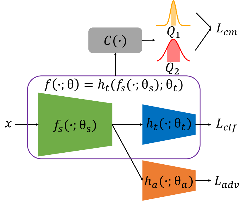
Back to our method. After defining , we add it to the traditional adversarially fair training (Ganin et al., 2016; Madras et al., 2018) loss function as a regularizer, in order to attain both in-distribution fairness and robust fairness. As illustrated in Figure 2, our model follows the same “two-head” structure as traditional adversarial learning frameworks (Ganin et al., 2016; Madras et al., 2018), where is the utility head for the target task, is the adversarial head to predict sensitive attributes, and is the shared backbone.222Thus the binary classifier , with . Suppose for each sample , the sensitive attribute is and the corresponding target label is , then our overall optimization problem can be written as:
| (7) |
where
| (8) | |||
| (9) |
is the cross-entropy loss function, and are trade-off hyperparameters, and is the number of training samples.
5 Experiments
| Method | In-distribution test set (Young and high visual quality face images) | Old face images with high visual quality | Young face images under sever JPEG compression | |
| Accuracy () | () | () | () | |
| In-distribution fairness | Robust fairness under distribution shifts | |||
| Normal | 85.76 | 37.42 | 40.52 | 43.01 |
| AdvDebias | 80.31 | 33.25 | 36.54 | 35.86 |
| LAFTR | 79.56 | 31.02 | 35.88 | 37.46 |
| CUMA | 80.26 | 31.52 | 33.26 | 33.12 |
| Method | In-distribution test set (Young and high visual quality face images) | Old face images with high visual quality | Young face images under sever JPEG compression | |
| Accuracy () | () | () | () | |
| In-distribution fairness | Robust fairness under distribution shifts | |||
| Normal | 85.76 | 43.56 | 42.03 | 40.15 |
| AdvDebias | 78.56 | 33.25 | 37.41 | 35.22 |
| LAFTR | 82.30 | 32.06 | 35.61 | 35.74 |
| CUMA | 81.06 | 31.15 | 33.06 | 32.52 |
5.1 Experimental Setup
Datasets and pre-processing
Experiments are conducted on three datasets widely used to evaluate machine learning fairness: Adult (Kohavi, 1996), and CelebA (Liu et al., 2015), and Communities and Crime (C&C) (Redmond & Baveja, 2002).333Traditional image classification datasets (e.g., ImageNet) are not directly applicable since they lack fairness attribute labels. Adult dataset has 48,842 samples with basic personal information such as education and occupation, where 30,000 are used for training and the rest for evaluation. The target task is to predict the person’s annual income, and we use “gender” (male or female) as the sensitive attribute. The features in Adult dataset are of either continuous (e.g., age) or categorical (e.g. sex) values. We use one-hot encoding on the categorical features and then concatenate them with the continuous ones. We use data whitening on the concatenated features. CelebA has over 200,000 images of celebrity faces, with 40 attribute annotations. The target task is to predict gender (male or female) and the sensitive attributes to protect are “chubby” and “eyeglasses”. We randomly select as training samples and as testing samples. All images are center-cropped and resized to , and pixel values are scaled to . C&C dataset has 1,994 samples with neighborhood population statistics, where 1,500 are used for training and the rest for evaluation. The target task is to predict violent crime per capita, and we use “RacePctBlack” (percentage of black population in the neighborhood) and “FemalePctDiv” (divorce ratio of female in the neighborhood) as sensitive attributes. All features in C&C dataset are of continous values in . To fit in the fairness problem setting, we binarilize the target and sensitive attributes with the top- largest value as the threshold (As a result and ). We also do data-whitening on C&C.
Models
For C&C and Adult datasets, we use two-layer MLPs for , and . Specifically, suppose the input feature dimension is , then the dimensions of hidden layers in and are and , respectively. has identical model structure with . For all three sub-networks, ReLU activation function and dropout layer with dropout ratio are applied between the two fully connected layers. For CelebA dataset, we use ResNet18 as backbone, where the first three stages are used as and the last stage (together with the fully connected classification layer) is used as . The auxiliary adversarial head has the same structure as .
Baseline methods
We compare CUMA with the following state-of-the-art in-distribution fairness algorithms. Adversarial debiasing (AdvDebias) (Zhang et al., 2018) is one of the most popular fair training algorithm based on adversarial training (Ganin et al., 2016). Madras et al. (2018) proposes a similar framework termed Learned Adversarially Fair and Transferable Representations (LAFTR), by replacing the cross-entropy loss used in (Zhang et al., 2018) with a group-normalized loss, which is shown to work better on highly unbalanced datasets. We also include normal (fairness-ignorant) training as a baseline.
Evaluation metric
We report the overall accuracy on all test samples in the original test sets. To measure in-distribution fairness, we use on the original test sets. To measure robust fairness under distribution shifts, we use on test sets with distribution shifts. See the following paragraph for the details in constructing distribution shifts.
Distribution shifts
Adult dataset contains US Census data collected before 1996. We use the 2014 and 2015 subset of Folktables dataset (Ding et al., 2021), which contain US Census data collected in 2014 and 2015 respectively, as the test sets with distribution shifts. This simulates the real-world temporal distributional shifts.
On CelebA dataset, we train the model on “young” face images. We use another “young” face images as in-distribution test set and “not young” face images as the test set with distribution shifts. This simulates the real-world scenario when the model is trained and used on people with different age groups. We also construct another test set with a different type of distribution shift, by applying strong JPEG compression on the original “young” test images, following (Hendrycks & Dietterich, 2019). This simulates the scenario when the model is trained on good quality images while the test images has poor visual quality.
For C&C dataset, we construct two artificial distribution shifts by adding random Gaussian and uniform noises, respectively, to the test data. Specifically, the categorical features in C&C dataset are first one-hot encoded and then whitened into float-value vectors, where noises are added. Both types of noises have mean and has standard derivation .
Implementation details
Unless further specified, we set the loss trade-off parameter to 1 in all experiments by default. We use Adam optimizer (Kingma & Ba, 2014) with initial learning rate and weight decay . The learning rate is gradually decreased to 0 by cosine annealing learning rate scheduler (Loshchilov & Hutter, 2016). On both Adult and C&C datasets, we train for epochs from scratch for all methods. On CelebA dataser, we first normally train a model for 100 epochs, and then finetune it for 20 epochs using CUMA. For fair comparison, we train for 120 epochs on CelebA for all baseline methods. The constant in Eq. (3) is set to by default.
| Method | The original C&C test set | With Gaussian Noise | With Uniform Noise | |
| Accuracy () | () | () | () | |
| In-distribution fairness | Robust fairness under distribution shifts | |||
| Normal | 89.05 | 63.22 | 60.13 | 64.21 |
| AdvDebias | 84.79 | 39.84 | 39.84 | 36.81 |
| LAFTR | 85.80 | 28.83 | 29.04 | 32.20 |
| CUMA | 85.20 | 28.17 | 28.69 | 27.11 |
| Method | The original C&C test set | With Gaussian Noise | With Uniform Noise | |
| Accuracy () | () | () | () | |
| In-distribution fairness | Robust fairness under distribution shifts | |||
| Normal | 89.05 | 54.74 | 56.41 | 54.60 |
| AdvDebias | 83.57 | 38.73 | 38.73 | 37.15 |
| LAFTR | 83.16 | 27.83 | 29.30 | 30.11 |
| CUMA | 83.39 | 27.57 | 27.70 | 28.35 |
5.2 Main Results
Experimental results on three datasets with different sensitive attributes are shown in Tables 2-6, where we compare CUMA with the baseline methods on different metrics as discussed in Section 5.1. “Normal” means standard training without any fairness regularization. All numbers are shown as percentages. Many intriguing findings can be concluded from the results.
First, we see that previous state-of-the-art fairness learning algorithms would be jeopardized if distributional shifts are present in test data. For example, on Adult dataset (Table 2), LAFTR achieves on in-distribution test set, while that number is increased to on the 2014 test set and on the 2015 test set, which is almost as unfair as the normally trained model. Similarly, on CelenA dataset with “Chubby” as the sensitive attribute (Table 3), LAFTR achieves on the original CelebA test set, while that number is increased to and under distribution shifts of user age and image quality, respectively.
Second, we see that CUMA achieves the best robust fairness under distribution shifts under all evaluated settings, while maintaining similar in-distribution fairness and overall accuracy. For example, on Adult dataset (Table 2), CUMA achieves and less than the second-best performer (AdvDebias) on the 2014 and 2015 Census dataset, respectively. On CelebA dataset (Table 3) with “Chubby” as the sensitive attribute, CUMA achieves and less than the second-best performers under distribution shifts of user age and image quality, respectively. Moreover, still in Table 3, CUMA and LAFTR achieve almost identical in-distribution fairness (the difference between their on original test set is ), CUMA keeps the fairness under distribution shifts (with only around increase in ), while the fairness achieved by LAFTR is significantly worse, especially under the image quality distribution shift, where the is increased by .
5.3 Ablation Study
In this section, we check the sensitivity of CUMA with respect to its hyper-parameters: the loss trade-off parameters and in Eq. (7) and in Eq. (3). Results are shown in Table 7. When fixing , the best trade-off between overall accuracy and robust fairness is achieved at round , which we use as the default . Varying the value of hardly affects the performance of CUMA.
| 0.1 | 1 | 10 | 0.1 | 1 | 10 | 0.1 | 1 | |
| Accuracy | 86.94 | 85.40 | 83.75 | 85.19 | 85.40 | 84.79 | 85.32 | 85.40 |
| with Gaussian noise | 66.51 | 28.74 | 33.16 | 38.85 | 28.74 | 27.95 | 30.56 | 28.74 |
5.4 Trade-off Curves between Fairness and Accuracy
For CUMA and both baseline methods, we can obtain different trade-offs between fairness and accuracy by setting the loss function weights (e.g., and ) to different values. For example, the larger , the better fairness and the worse accuracy. Such trade-off curves between fairness and accuracy of different methods are shown in Figure 3. The closer the curve to the top-left corner (i.e., with larger accuracy and smaller ), the better Pareto frontier is achieved. As we can see, our method achieves the best Pareto frontiers for both in-distribution fairness (left panel) and robust fairness under distribution shifts (middle and right panel).
 |
 |
 |
6 Conclusion
In this paper, we first observe the challenge of robust fairness: Existing state-of-the-art in-distribution fairness learning methods suffer significant performance drop under unseen distribution shifts. To solve this problem, we propose a novel robust fairness learning algorithm, termed Curvature Matching (CUMA), to simultaneously achieve both traditional in-distribution fairness and robust fairness. Experiments show CUMA achieves more robust fairness under unseen distribution shifts, without more sacrifice on either overall accuracies or the in-distribution fairness compared with traditional in-distribution fairness learning methods.
References
- Agarwal et al. (2018) Agarwal, A., Beygelzimer, A., Dudík, M., Langford, J., and Wallach, H. A reductions approach to fair classification. In International Conference on Machine Learning, pp. 60–69, 2018.
- Bahng et al. (2020) Bahng, H., Chun, S., Yun, S., Choo, J., and Oh, S. J. Learning de-biased representations with biased representations. In International Conference on Machine Learning, pp. 528–539, 2020.
- Bartlett et al. (2017) Bartlett, P., Foster, D. J., and Telgarsky, M. Spectrally-normalized margin bounds for neural networks. In Advances in Neural Information Processing Systems, 2017.
- Bińkowski et al. (2018) Bińkowski, M., Sutherland, D. J., Arbel, M., and Gretton, A. Demystifying MMD GANs. In International Conference on Learning Representations, 2018.
- Buolamwini & Gebru (2018) Buolamwini, J. and Gebru, T. Gender shades: Intersectional accuracy disparities in commercial gender classification. In Conference on Fairness, Accountability and Transparency, pp. 77–91, 2018.
- Calmon et al. (2017) Calmon, F. P., Wei, D., Vinzamuri, B., Ramamurthy, K. N., and Varshney, K. R. Optimized pre-processing for discrimination prevention. In International Conference on Neural Information Processing Systems, pp. 3995–4004, 2017.
- Creager et al. (2019) Creager, E., Madras, D., Jacobsen, J.-H., Weis, M., Swersky, K., Pitassi, T., and Zemel, R. Flexibly fair representation learning by disentanglement. In International Conference on Machine Learning, pp. 1436–1445, 2019.
- Dai & Brown (2020) Dai, J. and Brown, S. M. Label bias, label shift: Fair machine learning with unreliable labels. In NeurIPS Workshop, 2020.
- de Vries et al. (2019) de Vries, T., Misra, I., Wang, C., and van der Maaten, L. Does object recognition work for everyone? In IEEE Conference on Computer Vision and Pattern Recognition Workshops, pp. 52–59, 2019.
- Ding et al. (2021) Ding, F., Hardt, M., Miller, J., and Schmidt, L. Retiring Adult: New datasets for fair machine learning. arXiv preprint arXiv:2108.04884, 2021.
- Du et al. (2020) Du, M., Yang, F., Zou, N., and Hu, X. Fairness in deep learning: A computational perspective. IEEE Intelligent Systems, 2020.
- Dwork et al. (2012) Dwork, C., Hardt, M., Pitassi, T., Reingold, O., and Zemel, R. Fairness through awareness. In Innovations in Theoretical Computer Science Conference, pp. 214–226, 2012.
- Edwards & Storkey (2016) Edwards, H. and Storkey, A. Censoring representations with an adversary. In International Conference on Learning Representations, 2016.
- Ganin et al. (2016) Ganin, Y., Ustinova, E., Ajakan, H., Germain, P., Larochelle, H., Laviolette, F., Marchand, M., and Lempitsky, V. Domain-adversarial training of neural networks. Journal of Machine Learning Research, 17(1):2096–2030, 2016.
- Gretton et al. (2012) Gretton, A., Borgwardt, K. M., Rasch, M. J., Schölkopf, B., and Smola, A. A kernel two-sample test. Journal of Machine Learning Research, 13(1):723–773, 2012.
- Guo et al. (2018) Guo, Y., Zhang, C., Zhang, C., and Chen, Y. Sparse DNNs with improved adversarial robustness. In Advances in Neural Information Processing Systems, 2018.
- Hardt et al. (2016) Hardt, M., Price, E., and Srebro, N. Equality of opportunity in supervised learning. In Advances in Neural Information Processing Systems, 2016.
- Hashimoto et al. (2018) Hashimoto, T., Srivastava, M., Namkoong, H., and Liang, P. Fairness without demographics in repeated loss minimization. In International Conference on Machine Learning, pp. 1929–1938, 2018.
- Hendrycks & Dietterich (2019) Hendrycks, D. and Dietterich, T. Benchmarking neural network robustness to common corruptions and perturbations. International Conference on Learning Representations, 2019.
- Hendrycks et al. (2020) Hendrycks, D., Basart, S., Mu, N., Kadavath, S., Wang, F., Dorundo, E., Desai, R., Zhu, T., Parajuli, S., Guo, M., Song, D., Steinhardt, J., and Gilmer, J. The many faces of robustness: A critical analysis of out-of-distribution generalization. arXiv preprint arXiv:2006.16241, 2020.
- Hendrycks et al. (2021) Hendrycks, D., Zhao, K., Basart, S., Steinhardt, J., and Song, D. Natural adversarial examples. In IEEE Conference on Computer Vision and Pattern Recognition, 2021.
- Hwang et al. (2020) Hwang, S., Park, S., Kim, D., Do, M., and Byun, H. Fairfacegan: Fairness-aware facial image-to-image translation. In British Machine Vision Conference, 2020.
- Kamiran & Calders (2012) Kamiran, F. and Calders, T. Data preprocessing techniques for classification without discrimination. Knowledge and Information Systems, 33(1):1–33, 2012.
- Kingma & Ba (2014) Kingma, D. P. and Ba, J. Adam: A method for stochastic optimization. arXiv preprint arXiv:1412.6980, 2014.
- Kingma & Welling (2013) Kingma, D. P. and Welling, M. Auto-encoding variational bayes. arXiv preprint arXiv:1312.6114, 2013.
- Kohavi (1996) Kohavi, R. Scaling up the accuracy of naive-Bayes classifiers: A decision-tree hybrid. In International Conference on Knowledge Discovery and Data Mining, pp. 202–207, 1996.
- Li et al. (2017) Li, C.-L., Chang, W.-C., Cheng, Y., Yang, Y., and Póczos, B. MMD GAN: Towards deeper understanding of moment matching network. In International Conference on Machine Learning, 2017.
- Li et al. (2019) Li, T., Sanjabi, M., Beirami, A., and Smith, V. Fair resource allocation in federated learning. In International Conference on Learning Representations, 2019.
- Li & Vasconcelos (2019) Li, Y. and Vasconcelos, N. REPAIR: Removing representation bias by dataset resampling. In IEEE Conference on Computer Vision and Pattern Recognition, pp. 9572–9581, 2019.
- Li et al. (2015) Li, Y., Swersky, K., and Zemel, R. Generative moment matching networks. In International Conference on Machine Learning, pp. 1718–1727, 2015.
- Liu et al. (2015) Liu, Z., Luo, P., Wang, X., and Tang, X. Deep learning face attributes in the wild. In IEEE International Conference on Computer Vision, 2015.
- Loshchilov & Hutter (2016) Loshchilov, I. and Hutter, F. SGDR: Stochastic gradient descent with warm restarts. arXiv preprint arXiv:1608.03983, 2016.
- Madras et al. (2018) Madras, D., Creager, E., Pitassi, T., and Zemel, R. Learning adversarially fair and transferable representations. In International Conference on Machine Learning, pp. 3384–3393, 2018.
- Mandal et al. (2020) Mandal, D., Deng, S., Jana, S., and Hsu, D. Ensuring fairness beyond the training data. In NeurIPS, 2020.
- Martinez et al. (2020) Martinez, N., Bertran, M., and Sapiro, G. Minimax Pareto fairness: A multi objective perspective. In International Conference on Machine Learning, pp. 6755–6764, 2020.
- Miyato et al. (2018) Miyato, T., Maeda, S.-i., Koyama, M., and Ishii, S. Virtual adversarial training: a regularization method for supervised and semi-supervised learning. IEEE Transactions on Pattern Analysis and Machine Intelligence, 41(8):1979–1993, 2018.
- Moosavi-Dezfooli et al. (2019) Moosavi-Dezfooli, S.-M., Fawzi, A., Uesato, J., and Frossard, P. Robustness via curvature regularization, and vice versa. In IEEE Conference on Computer Vision and Pattern Recognition, pp. 9078–9086, 2019.
- Muñoz et al. (2016) Muñoz, C., Smith, M., and Patil, D. Big data: A report on algorithmic systems, opportunity, and civil rights. United States Executive Office of the President, 2016.
- Nagpal et al. (2019) Nagpal, S., Singh, M., Singh, R., and Vatsa, M. Deep learning for face recognition: Pride or prejudiced? arXiv preprint arXiv:1904.01219, 2019.
- Nam et al. (2020) Nam, J., Cha, H., Ahn, S.-S., Lee, J., and Shin, J. Learning from failure: De-biasing classifier from biased classifier. In Advances in Neural Information Processing Systems, 2020.
- Park et al. (2020) Park, S., Hwang, S., Hong, J., and Byun, H. Fair-VQA: Fairness-aware visual question answering through sensitive attribute prediction. IEEE Access, 8:215091–215099, 2020.
- Podesta et al. (2014) Podesta, J., Pritzker, P., Moniz, E. J., Holdren, J., and Zients, J. Big data: Seizing opportunities and preserving values. United States Executive Office of the President, 2014.
- Qiu et al. (2019) Qiu, Y., Leng, J., Guo, C., Chen, Q., Li, C., Guo, M., and Zhu, Y. Adversarial defense through network profiling based path extraction. In IEEE Conference on Computer Vision and Pattern Recognition, pp. 4777–4786, 2019.
- Quadrianto & Sharmanska (2017) Quadrianto, N. and Sharmanska, V. Recycling privileged learning and distribution matching for fairness. In Advances in Neural Information Processing Systems, 2017.
- Quadrianto et al. (2019) Quadrianto, N., Sharmanska, V., and Thomas, O. Discovering fair representations in the data domain. In IEEE Conference on Computer Vision and Pattern Recognition, pp. 8227–8236, 2019.
- Redmond & Baveja (2002) Redmond, M. and Baveja, A. A data-driven software tool for enabling cooperative information sharing among police departments. European Journal of Operational Research, 141(3):660–678, 2002.
- Rezaei et al. (2021) Rezaei, A., Liu, A., Memarrast, O., and Ziebart, B. D. Robust fairness under covariate shift. In AAAI, pp. 9419–9427, 2021.
- Sarhan et al. (2020) Sarhan, M. H., Navab, N., Eslami, A., and Albarqouni, S. Fairness by learning orthogonal disentangled representations. In European Conference on Computer Vision, pp. 746–761, 2020.
- Shankar et al. (2017) Shankar, S., Halpern, Y., Breck, E., Atwood, J., Wilson, J., and Sculley, D. No classification without representation: Assessing geodiversity issues in open data sets for the developing world. In Advances in Neural Information Processing Systems Workshop, 2017.
- Singh et al. (2021) Singh, H., Singh, R., Mhasawade, V., and Chunara, R. Fairness violations and mitigation under covariate shift. In FAccT, pp. 3–13, 2021.
- Smuha (2019) Smuha, N. A. The EU approach to ethics guidelines for trustworthy artificial intelligence. Computer Law Review International, 20(4):97–106, 2019.
- Taori et al. (2020) Taori, R., Dave, A., Shankar, V., Carlini, N., Recht, B., and Schmidt, L. Measuring robustness to natural distribution shifts in image classification. In Advances in Neural Information Processing Systems, 2020.
- Wadsworth et al. (2018) Wadsworth, C., Vera, F., and Piech, C. Achieving fairness through adversarial learning: an application to recidivism prediction. arXiv preprint arXiv:1807.00199, 2018.
- Wang et al. (2019) Wang, T., Zhao, J., Yatskar, M., Chang, K.-W., and Ordonez, V. Balanced datasets are not enough: Estimating and mitigating gender bias in deep image representations. In IEEE International Conference on Computer Vision, pp. 5310–5319, 2019.
- Weng et al. (2018) Weng, T.-W., Zhang, H., Chen, P.-Y., Yi, J., Su, D., Gao, Y., Hsieh, C.-J., and Daniel, L. Evaluating the robustness of neural networks: An extreme value theory approach. In International Conference on Learning Representations, 2018.
- Wilson et al. (2019) Wilson, B., Hoffman, J., and Morgenstern, J. Predictive inequity in object detection. arXiv preprint arXiv:1902.11097, 2019.
- Yan et al. (2021) Yan, H., Zhang, J., Niu, G., Feng, J., Tan, V. Y., and Sugiyama, M. CIFS: Improving adversarial robustness of cnns via channel-wise importance-based feature selection. arXiv preprint arXiv:2102.05311, 2021.
- Zhang et al. (2018) Zhang, B. H., Lemoine, B., and Mitchell, M. Mitigating unwanted biases with adversarial learning. In AAAI Conference on AI, Ethics, and Society, pp. 335–340, 2018.
- Zhang et al. (2021) Zhang, W., Bifet, A., Zhang, X., Weiss, J. C., and Nejdl, W. FARF: A fair and adaptive random forests classifier. In PACKDD, pp. 245–256, 2021.
- Zhao et al. (2017) Zhao, J., Wang, T., Yatskar, M., Ordonez, V., and Chang, K.-W. Men also like shopping: Reducing gender bias amplification using corpus-level constraints. arXiv preprint arXiv:1707.09457, 2017.