How Reliable are University Rankings?
Abstract
University or college rankings have almost become an industry of their own, published by US News & World Report (USNWR) and similar organizations. Most of the rankings use a similar scheme: Rank universities in decreasing score order, where each score is computed using a set of attributes and their weights; the attributes can be objective or subjective while the weights are always subjective. This scheme is general enough to be applied to ranking objects other than universities. As shown in the related work, these rankings have important implications and also many issues. In this paper, we take a fresh look at this ranking scheme using the public College dataset; we both formally and experimentally show in multiple ways that this ranking scheme is not reliable and cannot be trusted as authoritative because it is too sensitive to weight changes and can easily be gamed. For example, we show how to derive reasonable weights programmatically to move multiple universities in our dataset to the top rank; moreover, this task takes a few seconds for over 600 universities on a personal laptop. Our mathematical formulation, methods, and results are applicable to ranking objects other than universities too. We conclude by making the case that all the data and methods used for rankings should be made open for validation and repeatability.
1 Introduction
Rankings of higher education institutions (universities for short) have almost become an industry of its own [33]. Most of the rankings use a similar methodology: Select a set of numeric attributes and a numeric weight for each attribute, then compute a final numeric score as the sum of the products of each attribute with its weight. The weight of an attribute determines the amount of contribution the attribute makes to the final score. For the final ranking, the universities are ranked in their decreasing score order.
This generic ranking methodology is simple enough that it has been applied to ranking all kinds of objects, from universities to hospitals to cities to countries [41], e.g., see [40, 59, 60] for the rankings methodologies for objects other than universities: Places to live, hospitals, and countries. As a result, even though our focus in this study is universities, the findings are applicable to other areas where this generic ranking methodology is used.
There are many questions that have been explored about this ranking methodology in general and university rankings in particular. For example, why a given attribute is selected, whether a given attribute has the correct or most up-to-date value, why an attribute is weighted more than another one, what impact the opinion-based attributes have on the final score, whether or the impact of these rankings in student choices is warranted, whether or not a university should incentivize their admins to improve their rank with a given ranking, whether or not a university games these rankings when they share their data, etc. There is a rich body of related work exploring many of these issues, as explored in our related work section. There is also an international effort that has provided a set of principles and requirements (called the Berlin Principles [30]) to improve rankings and the practical implementations of the generic ranking methodology.
We start our study in § 2 by applying the steps of a generic ranking methodology codified in ten steps in an OECD handbook [41], to a public dataset, called the College dataset, about more than a 1,000 US higher education institutions. Though the College dataset was created in the year 1995, the resulting ranking shows good alignment with the most recent rankings from the well-known ranking organizations.
These well-known ranking organizations are the US News & World Report (USNWR) [66], Quacquarelli Symonds (QS) [64], Times Higher Education (THE) [65], and ShanghaiRanking Consultancy (SC) [62]. We present the methodologies of and the most recent rankings from these organizations in § 3. We also present two recent rankings of universities in the computer science field, created by two groups of academicians in the computer science department of a few US universities.
We give a comprehensive but not exhaustive review of the rankings literature, including the related Economics literature, in § 4. We lean towards providing references to survey or overview papers as well as entry points to subfields so that the interested readers can go deeper if they so desire.
We follow this by introducing the mathematical formulation that underlies the generic ranking methodology. The mathematical formulation uses concepts from linear algebra and integer linear programming (ILP).
The main part of this paper is presented in § 6. We formulate and solve six problems in this section. The main vehicle we use in our formulation of these problems is the integer linear programming. The ILP programs for these problems take a few seconds to both generate and run for over 600 universities on a personal laptop.
In the first problem in § 6.1, we explore the existence of different rankings using Monte Carlo (randomized) simulation. We show that there are many possible rankings and somewhat naturally there are more than one university that can attain the top rank.
In the second problem in § 6.2, we do the same exploration but using the ILP for optimality. We confirm and go beyond the findings of the simulation: We verify that many universities can be moved to the top rank.
These two problems may show existence using weights that may not be appealing to a human judge, e.g., they may be widely different from each other, possibly yielding more than deserved impact on the final score. In the third problem in § 6.3, we rectify this situation and derive appealing weights. We replicate the findings of the first two problems using these new weights too.
These three problems show that there are many universities that can attain the top rank, though not every university can do so. Then a natural next question is how to find the best rank that each university can attain. We attack this question in the fourth problem in § 6.4.
The first four problems always involve attribute weights, as in the generic ranking methodology. In the fifth problem in § 6.5, we explore a way of generating rankings without weights, which uses the Kemeny rule [20]. This no-weights ranking approach eliminates many of the issues associated with weight selection.
In the sixth and the last problem in § 6.6, we show how a given university can improve its rank in a weight-based ranking. We show that drastic rank improvements are possible by few attribute value changes.
In this paper our main thesis is that university rankings as commonly done today and somehow proposed as unique with so much fanfare are actually not reliable and can even be easily gamed. We believe our results via these six problems provide strong support to this thesis. This thesis applies especially to the universities at the top rank. We show in multiple ways that it is relatively easy to move multiple university to the top rank in a given ranking. As we mentioned above, our findings are applicable to areas where objects other than universities are ranked. In § 7, we provide a discussion of these points together with a few recommendations.
One unfortunate aspect of the rankings from the four well-known rankings organizations is that their datasets and software code used for their rankings are not in the public domain for repeatability. We wanted to change this so we have posted our datasets and the related software code in a public code repository [16]. We hope the well-known rankings organizations too will soon share their latest datasets and the related software code in the public domain.
2 A Ranking Exercise Using a Public Dataset
Rankings of higher education institutions were first started by the U.S. Bureau of Education in 1870 and have been done by multiple other organizations since; however, it can be argued that the current rankings industry has been ignited by the U.S. News and World Report’s first “America’s Best Colleges” ranking in 1983 [33]. Today, there are many rankings around the world, some of which are the well-known worldwide rankings and some are country specific [63]. The four well-known rankings that we will cover in § 3 are the US News & World Report (USNWR), Quacquarelli Symonds (QS), Times Higher Education (THE), and ShanghaiRanking Consultancy (SC).
In the sequel, for simplicity, we will use the term “university” to refer to a university, a college, or a higher education institution, regardless of the university is private or public, American or international, i.e., one that belongs to another country.
Rankings are also common in areas other than higher education. For example, there is a huge literature in Economics and related fields on comparing countries on over 100 different human progress measures, the most famous of which is probably the Human Development Index of the United Nations [41, 68]. These rankings use a ranking methodology very similar to the one used for university rankings; as a result, many of the results from this literature, including the pitfalls, are applicable to university rankings.
As comprehensively outlined in the OECD rankings handbook [41], a typical ranking methodology follows ten steps from step 1 to step 10, after the selection of the input dataset, which we will refer to as step 0. We will apply these ten steps to a ranking exercise of our own with the College dataset. All the experiments reported in this paper were done on this dataset.
2.1 Step 0: Gathering the Input Data
In general, there are three basic sources of the input data for university ranking [56]:
-
a)
surveys of the opinions of various stakeholders such as university or high school administrators;
-
b)
independent third parties such as government agencies; and
-
c)
university sources.
The last source is now standardized under the initiative called the “Common Data Set Initiative” [67]. A simple web search with a university name followed by the query “Common Data Set” will return many links to these data sets from many universities. Note that among these three data sources, the survey data is inherently subjective while the other two are supposed to be objective, although unfortunately some intentional alteration of data by university sources have been observed [46].
Our data source fits into category b above: The College dataset [52] is part of the StatLib datasets archive, hosted at the Carnegie Mellon University; it contains data about many (1,329 to be exact) but not all American higher education institutions. Its collection in 1995 was facilitated by the American Statistical Association. The two data sources are Association of American University Professors (AAUP) and US News & World Report (USNWR), which contribute 17 and 35 attributes, respectively, per university. There are many attributes with missing values for multiple universities. See [52] for the meaning of each attribute. All the attributes in this dataset are objective.

With the attributes and weights we selected, as detailed below, we generated the top 20 universities as shown in Fig. 1. We hope the reader can appreciate that this ranking is a reasonable one to the extent it aligns well with the well-known rankings, to be discussed in a bit below.
One question that may come to the reader’s mind could be the reason for selecting this dataset and the relevance of this fairly old dataset to the present. For the reason question, we wanted to make sure that we choose a standard dataset that is available to all who want to replicate our results; moreover, we do not have access to the latest datasets used by the well-known rankings organizations. For the relevance question, we ask the reader to review our mathematical and problem formulations and convince themselves that our results are applicable to any dataset containing a set of objects to rank using their numerical attributes.
2.2 Step 1: Developing a Theoretical or Conceptual Framework
We have universities in some ranking, each of which has the same attributes (also called variables or indicators in the Economics literature) with potentially different values. We will use to index universities and to index attributes. Each attribute of the th university is associated with the same real-number weight . The score of the th university is a function of the attributes and weights of the university as
| (1) |
where the functions and usually reduce to the identity function resulting in the following sum-of-products form:
| (2) |
where the th weight determines the contribution of the th attribute to the final score.
A ranking of universities is a sorting of scores in decreasing order such that the “top” ranked or the “best” university is the university with the highest score or the one at rank 1. Later in § 6.5 we will discuss how to rank universities without weights, in which case the ranking does not use scores.
Since this framework is well detailed in the mathematical formulation section in § 5, we will keep this section short. Also see the weighting and aggregation section (§ 2.7) on how the attributes and weights are manipulated for ranking.

2.3 Step 2: Selecting Attributes
In general, the attributes for ranking or as indicators of quality in higher education can be grouped into the following four categories [24]:
-
a)
beginning characteristics, which cover the characteristics of the incoming students such as test scores or high school ranking;
-
b)
learning inputs, which cover factors that help affect the learning experiences of students such as the financial resources of the university;
-
c)
learning outputs, which cover the skill sets or any other attributes of graduates; and
-
d)
final outcomes, which cover the outcomes of the educational system and what the students achieve in the end such as employment, income, and job satisfaction.
It may be argued that category d is what matters most but most of the current rankings focus on categories a and b because category d and to some extent category c are difficult to measure continuously. Our attributes due to what we can find in our dataset also fall into categories a and b.
We prepared our dataset in two steps: 1) we joined the two source datasets from AAUP and USNWR using the FICE code, a unique id per university assigned by the American Federal Government. This generated 1,133 universities. 2) We selected 20 attributes out of the 52 total, including the name and the state of the university. We then eliminated any university with a missing value for any of the selected attributes. This resulted in 603 universities.
The selected 20 attributes are: University, state, instructional expenditure per student (1), in-state tuition (1), room and board costs (1), room costs, board costs (1), additional fees (1), estimated book costs (1), estimated personal spending (1), number of applications received (2), number of applicants accepted (2), number of new students enrolled (3), percent of new students from the top 10% of their high school class (4), percent of new students from the top 25% of their high school class (5), percent of faculty with terminal degree (6), percent of faculty with PhDs (5), student/faculty ratio (8), graduation rate (9), percent of alumni who donate (10), number of full professors (11), and number of faculty in all ranks (11). The number in parenthesis indicates that the corresponding attribute is used to derive the th attribute in Fig. 2.
Why did we choose only 20 attributes out of the 52 total? Two reasons: We wanted to use as many attributes as possible for each university; we also wanted to make sure that the final list of attributes used in ranking are comparable in the following senses:
-
1.
Every final attribute is either a percentage or a ratio. This ensures that they are comparable in magnitude.
-
2.
For every final attribute, a university with a higher value should be regarded by a prospective student as “better” than another university with a lower value.
Taking these two into account, we could not select more than 20 initial attributes from the 52 total. We then converted these 20 attributes into a final list of 11 attributes (see Fig. 2), not counting the name and the state of the university, using the following thought process that we think a reasonable student would potentially go through:
“I, the student, want to go to a university
-
:
that spends for me far more than what it costs me in total (so that I get back more than what I put in);
-
, :
that is desired highly by far more students that it can accommodate (so that I get a chance to study with top students);
-
, :
that attracts the top students in their graduating class (so that I get a chance to study with top students);
-
, :
that has more faculty with PhDs or other terminal degrees in their fields (so that I get taught by top researchers or teachers);
-
:
that has a smaller student to faculty ratio (so that I can get more attention from professors);
-
:
that has a higher graduation rate (so that I can graduate more easily);
-
:
that has more of its alumni donating to the university (so that more financial resources are available to spend on students); and
-
:
that has more of its classes taught by full professors (so that I get taught by top researchers or teachers).”
Here the spend above indicates the total instructional expenditure by the university per student and the cost to a student above covers the tuition, room and board, fees, books, and personal expenses.
We hope the arguments made above look reasonable and we expect them to be at least directionally correct. For example, a top researcher may not be a top teacher but it feels reasonable to us to assume that with a solid research experience there is some correlation towards better qualifications to teach a particular subject.
The reader may or may not agree with this attribute selection process but that is exactly one of the points of this paper: There is so much subjectivity creeping in during multiple steps of the ranking process. Later we will show how to remove some of this bias.
2.4 Step 3: Imputation of Missing Data
We then realized that we could easily repair some missing values: a) if the value of the attribute “room and board costs” is missing, it can easily be calculated by the sum of the values of the attributes “room costs” and “board costs” if both exist; b) University of California campuses have very similar tuitions and fees, so we substituted any missing value with the average of the remaining values; c) For Stanford University, the values of the attributes “additional fees” and “percent of faculty with PhDs” were missing so we replaced them with the values we were able to find or calculate after some web searching. After these few repairs, we were able to increase the number of universities very modestly, from 603 to 609 to be exact, in our input dataset. We note that these repairs were not necessary to reach our conclusions but if not done, well-regarded universities like Stanford University and most of the University of California campuses would have been missing from the final ranking.
2.5 Step 4: Multivariate Analysis
Using techniques such as principal component analysis or factor analysis, this step looks at the underlying structure via the independent components or factors of the attribute space. We will skip this step for our dataset as this step is not highly relevant to the theme of this paper.
2.6 Step 5: Normalization of Data
Normalization ensures that each attribute falls into the same interval, usually , in magnitude. This is required for one of the ways of computing the final score for a university, the arithmetic mean method [41, 55].
In our case, every attribute except for the “university spend to student cost ratio” already falls in the unit interval . This is because all our attributes are percentages or ratios by construction. To minimize the impact of normalization on ranking, we decided to normalize the only exception (i.e., the university spend to student cost ratio) using the following formula (called the min-max normalization [41]):
| (3) |
where and are the maximum and minimum values for the attribute in question among the selected universities.

2.7 Step 6: Weighting and Aggregation
As mentioned earlier, each university has the same attributes but with potentially different values. Each attribute is paired with a weight , which is the same across all universities. These attribute and university pairs are manipulated in one of the following ways to generate a score so that universities can be ranked by their scores.
The weighted arithmetic mean formula. The score of the th university is equal to
| (4) |
where due to normalization or by construction the sum of the weights in the denominator is equal to 1, i.e., .
The weighted geometric mean formula. The score of the th university is equal to
| (5) |
where due to normalization or by construction the sum of the weights in the denominator is equal to 1, i.e., . Here and are the exponential and natural logarithm functions, respectively.
Between these, the former formula is more common although the latter is proven to be more robust [55]. The former formula is a sum-of-products formula referred to by many other names in especially the Economics literature such as “the composite index” (the most common), “the weight-and-sum method”, “the composite indicator”, “the attribute-and-aggregate method”, “the simple additive weighting”, or “the weighted linear combination”, e.g. see [56]. When the sum of the weights is unity, the formula is also equivalent to the dot product of the attribute and weight vectors.
Now we know how to compute a score per university but how do we select the weights? There are at least three ways of selecting weights [25, 41]: a) data driven such as using principal component analysis; b) normative such as public or expert opinion, equal weighting, arbitrary weighting; and c) hybrid weighting. We will use the normative weighting scheme as follows.
-
1.
Non-uniform weighting. We use the student persona in § 2.3 to select 20 weights subjectively. Fig. 2 shows the 11 weights derived out of these 20. Here is our heuristic for selecting the 20 weights: By ranking the universities per attribute, we looked at the top 10 universities in rank visually and how they align with the top 10 from the four well-known rankings. We then classified the attributes into three strength categories: High, medium, low, where high means the resulting ranking aligns well (again subjectively) with the top 10 from the four rankings whereas medium and low show less alignment. Finally, we decided to double the weight for each increment in strength. Note that we give the highest weights to the school selectivity (via the acceptance rate (inverted)) and the student selectivity (via the percent of students from top 10 in high school).
-
2.
Uniform weighting. We assign the same weight of 1 to every attribute. This removes any potential bias due to weight differences among attributes but it has its own critiques, e.g., see [25].
-
3.
Random weighting. We assign a uniformly random weight to each attribute subject to the constraint that the sum of the weights is equal to 1. Random weighting and its consequences are explored in § 6.1.
Fig. 3 compares the ranking of the top 20 in our dataset with respect to different weighting schemes, the arithmetic vs. geometric formula and the non-uniform vs. the uniform weights. Note that although the few universities are the top in each ranking, some universities such as “University of California (UC), Berkeley” have significant differences in their rankings. This observation provides another support for our claim that weighted rankings are not robust.
A word of caution is that even though our discussion above may imply that our top 20 ranking is similar to the ones by the well-known rankings in part by design, we will later prove by various random or deterministic weight selections, including no weights, that the top 20 rankings are still similar. In other words, the design heuristic we use above is for convenience only and it is immaterial to the conclusions of this paper.
2.8 Steps 7-9: Robustness, Sensitivity, and Data Analysis
We will cover this in the experimental results.
2.9 Step 10: Visualization of the Results
Our top 20 ranking from the College dataset is shown in Fig. 1. Our dataset and this top 20 ranking both include liberal arts colleges; the four rankings organizations usually have a separate ranking for liberal arts colleges. In this figure, we show the attribute values and the final unnormalized score. The last row shows our weights chosen for this ranking. We hope the readers can convince themselves that the resulting rankings, both non-uniform and uniform cases, seem reasonable and look in close alignment with the four well-known rankings (also see the argument in the last paragraph in the section for Step 6).
All in all, we hope we have provided a reasonable illustration of a ranking process in this section. As we repeatedly mention, our mathematical formulation and conclusions are not specific to this dataset.
3 The Four Well-known Rankings
We now briefly discuss the four well-known rankings in this section. For each ranking, we provide a very brief history, its ranking methodology with the list of the latest attributes and their weights, and the top 10 universities. This section covers the rankings of universities in the aggregate as well as in Computer Science.

3.1 U.S. News & World Report (USNWR) Rankings
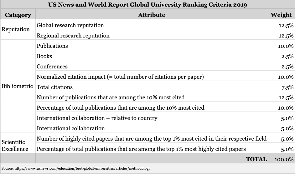
U.S. News & World Report (USNWR) rankings have been active since 1985 [66]. The attributes and weights of the latest ranking methodology are shown in Fig. 4 for US national ranking and in Fig. 5 for global ranking.
The national ranking has six categories of attributes, which are 13 in total, and the weights range from 1% to 22%. About 20% of the total weight, i.e., the “peer assessment” attribute, is opinion based. The global ranking has three categories of attributes, which are also 13 in total, and the weights range from 2.5% to 12.5%. About 25% of the total weight, i.e., the research reputation attributes, is opinion based.
More details about the methodology is available at [38] and [39] for the national and global rankings, respectively. The latest rankings using this methodology are available at [58] and [57] for the national and global rankings, respectively.

3.2 Quacquarelli Symonds (QS) Rankings
The Quacquarelli Symonds (QS) rankings have been active since 2004 [64]. Between 2004 and 2010, these rankings were done in partnership with Times Higher Education (THE). Since 2010, QS rankings have been produced independently. The attributes and weights of the latest ranking methodology are shown in Fig. 6; it has five categories of attributes, which are seven in total. The weights range from 5% to 20%. At least 50% of the total weight is opinion based under the “academic reputation” and “employer reputation” categories. More details about the methodology is available at [45]. The latest rankings using this methodology are available at [44].

3.3 Times Higher Education (THE) Rankings
The Times Higher Education (THE) rankings have been active since 2004 [65]. Between 2004 and 2010, these rankings were done in partnership with QS. Since 2010, THE rankings have been produced independently. The attributes and weights of the latest ranking methodology are shown in Fig. 6; it has five categories of attributes, which are 13 in total. The weights range from 2.25% to 30%. At least 33% of the total weight is opinion based under the “reputation survey” attributes. More details about the methodology is available at [54]. The latest rankings using this methodology are available at [53].

3.4 ShanghaiRanking Consultancy (SC) Rankings
The ShanghaiRanking Consultancy (SC) rankings have been active since 2003 [62, 35]. Between 2003 and 2008, these rankings were done by Shanghai Jiao Tong University. Since 2009, these rankings have been produced independently. The attributes and weights of the latest ranking methodology are shown in Fig. 8; it has four categories of attributes, which are six in total. The weights range from 10% to 20%. No part of the total weight is directly opinion based. More details about the methodology is available at [50]. The latest rankings using this methodology are available at [49].

3.5 The Top 10 Overall Rankings Comparison
To illustrate the differences between rankings, Fig. 9 shows the top 10 overall rankings of the US universities. In this figure, the first column is the reference for this table: USNWR national ranking. The next four rankings are USNWR global ranking, and the other three well-known rankings. In the column “Kemeny”, we present a ranking (called the Kemeny ranking) using the Kemeny rule, which minimizes the disagreements between the first four rankings and the final ranking [20]. Finally, in the column “Average”, we present a ranking using the average of the ranks over the first five columns.
Fig. 9 already illustrates the wide variation between these rankings: a) there is no university that has the same rank across all these rankings; b) there is not even an agreement for the top university; c) some highly regarded universities, e.g., UC Berkeley, are not even in top 10 in these rankings; and d) the two USNWR rankings of the same universities do not agree. The last row shows the difference between each ranking and the Kemeny ranking, where the difference is computed using Spearman’s footrule [15, 51], which is nothing more than the sum of the absolute differences between pairwise ranks. The distance shows that the rankings closer to the Kemeny ranking in decreasing order are the following rankings: Average, USNWR national, Times THE, QS, Shanghai SC, and USNWR global.
It is instructive to see the top ranked university in each ranking: Princeton University in USNWR national ranking, Harvard University in USNWR global ranking and SC ranking, Massachusetts Institute of Technology in QS ranking and Kemeny ranking, Stanford University in THE ranking, Harvard University in SC ranking and the average ranking. The top ranked university in these rankings may also change from year to year. These disagreements even for the top ranked university hopefully convinces the readers about the futility of paying attention to the announcements of the top ranked university from any rankings organization.

3.6 The Top 10 Computer Science Rankings Comparison
To illustrate the differences between rankings hopefully better, Fig. 10 gives the top 10 university rankings for computer science. Three words of caution here are a) that these rankings organizations use different titles for their computer science rankings (USNWR: “Computer and Information Sciences”, QS: “Computer Science and Information Systems”, THE: “Computer Science”, SC: “Computer Science and Engineering”); b) that due to these different titles these rankings possibly cover more than computer science; and c) that it is not clear what changes these organizations made in their generic ranking methodologies for computer science and, for that matter, for other subjects or areas.
The first two columns in Fig. 10 are by CSRankings [5] and CSMetrics [23], respectively, two computer science focused rankings developed and maintained by academicians in computer science [22]. These two rankings also align well with our own experiences as computer scientists. For the sake of simplicity, we will refer to them as the “academic” rankings.
These academic rankings are mainly based on citations in almost all the venues that matter to computer science. The central premise of these rankings is “to improve rankings by utilizing more objective data and meaningful metrics” [22]. These rankings intent to follow the best practices set by the Computing Research Association (CRA): “CRA believes that evaluation methodologies must be data-driven and meet at least the following criteria: a) Good data: have been cleaned and curated; b) Open: data is available, regarding attributes measured, at least for verification; c) Transparent: process and methodologies are entirely transparent; and d) Objective: based on measurable attributes.” These best practices are the reason for these sites declaring themselves as GOTO-ranking compliant, where GOTO stands for these four criteria. For computer science rankings, a call to ignore the computer science ranking by USNWR was made by the CRA due to multiple problems found with the ranking [3].
Note in Fig. 10 the significant differences among the rankings. As mentioned above, we agree with the academic rankings. However, it is difficult to agree with the ranks assigned to some universities in the other rankings. For example, it is difficult for us to agree with Carnegie Mellon University having rank 25 in USNWR and University of California, Berkeley having rank 118 in THE. Any educated computer scientist would agree that these two universities are definitely among the best in computer science. These two examples alone show the unreliability of the “non-academic” rankings at least for computer science.
4 Related Work
There is a huge literature on rankings, especially in the Economics literature for rankings of countries for various well-being measures. As a result, we cannot be exhaustive here; we will instead refer to a fairly comprehensive set of key papers that are mainly overview or survey papers or papers that are directly relevant to our work.
Recall the following acronyms that we defined above for the four well-known rankings organizations: The US News & World Report (USNWR), Quacquarelli Symonds (QS), Times Higher Education (THE), and ShanghaiRanking Consultancy (SC).
[33] gives a history of rankings. [41] is the de facto bible of all things related to composite indices. Although the focus is on well-being indices for populations and countries, the techniques are readily applicable to university rankings, as we also briefly demonstrated in this paper. [56] surveys 18 rankings worldwide. It acknowledges that there is no single definition of quality, as seen by the different sets of attributes and weights used across these rankings. It recommends quality assurance to enable better data collection and reporting for improved inter-institutional comparisons.
[29] provides an insider view of USNWR rankings. [35] is a related paper but on SC rankings. [48], though focusing on SC and THE only, follows a general framework that can be used to to compare any two university rankings. It finds out that SC is only good for identifying top performers and only in research performance, that THE is undeniably biased towards British institutions and inconsistent in the relation between subjective and objective attributes. [8] proposes a critical analysis of SC, identifies many problems with SC, and concludes that SC does not qualify as a useful guide to neither academic institutions nor parents and students.
[21] presents and criticizes the arbitrariness in university rankings. [61] focuses on the technical and methodological problems behind the university rankings. By revealing almost zero correlation between the expert opinions and bibliometric outcomes, this paper casts a strong doubt on the reliability of expert-based attributes and rankings. This paper also argues that a league of outstanding universities in the world may not exceed 200 members, i.e., any ranks beyond 200 are potentially arbitrary. [10] presents a good discussion of the technical pitfalls of university ranking methodologies.
[13] provides guidelines on how to choose attributes. [25] reviews the most commonly used methods for weighting and aggregating, including their benefits and drawbacks. It proposes a process-oriented approach for choosing appropriate weighting and aggregation methods depending on expected research outcomes. [19] categorizes the weighting approaches into data-driven, normative, and hybrid and then discusses a total of eight weighting approaches along these categories. It compares their advantages and drawbacks.
[4] uses Kemeny rule based ranking to avoid the weight imprecision problem. [47] provides a comparative study of how to provide rankings without explicit and subjective weights. These rankings work in a way similar to Kemeny rule based ranking.
[27] provides a synopsis of the choices available for constructing composite indices in light of recent advances. [42] provides a literature review and history on research rankings and proposes the use of bibliometrics to strengthen new university research rankings.
[34] provides an example of how to game the rankings system, with multiple quotes from USNWR and some university presidents on how the system works. [32] presents a way to optimize the attribute values to maximize a given university’s rank in a published ranking.
[17, 18] construct a model to clarify the incentives of the ranker, e.g., USNWR, and the student. They find the prestige effect pushing a ranker into a ranking away from student-optimal, i.e., not to the advantage of the student. They discuss why a ranker chooses the attribute weights in a certain way and why they change them over time. They also present a student-optimal ranking methodology. [37] exposes the games business school play whether or not to reveal their rankings.
[36] provides the casual impact of rankings on application decisions, i.e., how a rank boost or decline of a university affect the number of applications the university gets in the following year.
University rankings are an instance of multi-objective optimization. [12] provides a survey of such systems spanning many different domains, including university rankings. [28] presents applications to ranking in databases.
In summary, rankings like many things in life have their own pros and cons [26]. The pros are that they in part rely on publicly available information [1]; that they bring attention to measuring performance [1]; that they have provided a wake-up call, e.g., in Europe [1], for paying attention to the quality of universities and providing enough funding for them due to the strong correlation between funding and high rank; that they provide some guidance to students and parents in making university choices; that they use easily understandable attributes and weights and a simple score-based ranking.
The cons are unfortunately more than the pros. The cons are that data sources can be subjective [61], can be and has been gamed [46], can be incomplete; that attributes and weights sometimes seem arbitrary [1, 43]; that weights accord too little importance to social sciences and humanities [1]; that many operations on attributes and weights affect the final rankings [27]; that many attributes can be highly correlated [43]; that there is no clear definition of quality [56]; that rankings encourage rivalry among universities and strengthen the idea of the academic elite [61]; that rankings lead to a “the rich getting richer” phenomenon due to highly ranked universities getting more funding, higher salaries for their admin staff, more demand from students, and more favorable view of quality in expert opinions [61]; that assigning credit such as where an award was given vs. where the work was done is unclear [61]; that expert opinions are shown to be statistically unreliable and yet some well-known ranking organizations still use them [61]; that even objective bibliometric analysis has its own issues [61]; that some rankings such as THE have undeniable bias towards British universities [48]; and that the current rankings cannot be trusted [8, 21, 22].
The current well-known rankings have created their own industry and they have strong financial and other incentives to continue their way of presenting their own rankings [18]. There are initiatives to close many drawbacks of the current rankings such as the “Common Data Set Initiative” to provide publicly available data directly from universities [9], Computer Science rankings created by people who know Computer Science as in academicians from Computer Science [22], a set of principles and requirements (called the Berlin Principles) that a ranking needs to satisfy to continuously improve [30], an international institution to improve the rankings methodology [31], extra validation steps and prompt action by the current rankings organization against gaming [29, 46]. In short, there is hope but it will take time to reach a state where many of the pros have been eliminated.
5 Mathematical Formulation
We have objects to rank. Objects are things like universities, schools, and hospitals. A ranking is presented to people to select one of. Each object has numerical attributes from to , index with . We can use the matrix to represent the objects and their attributes, one row for each thing and one column for each attribute.
| (6) |
We have unknown numerical coefficients from to in the vector .
| (7) |
where each represents a weight for the attribute for some . Each weight is non-negative. The same weights are used for every row of attributes. The sum of the weights is set to 1 due to normalization.
For each object , we compute a score as
| (8) |
or in the matrix form
| (9) |
where is the matrix of the known attributes and is the set of unknown weights, both as defined above. Recall from § 2.7, the score formula above is the arithmetic mean formula, and the scores can also be computed using the geometric mean formula. Note that is a matrix-vector multiplication. Also note that setting each weight in to 1 is the uniform weight case.
Fig. 1 illustrates the attributes, weights, scores, and ranks for the top 20 universities from the College dataset. The attributes across all 20 rows and 11 columns represent the matrix for the top 20 universities only; the actual matrix has over 600 rows. The last row in this table represents the vector of 11 weights we assigned for this ranking. The last two columns represent the vector of scores and the ranks for each university.
Ordering. The top ranking, like the top 20 in Fig. 1, is an ordering of these universities in decreasing score, i.e.,
| (10) |
which we will refer as the score ordering constraint. Another form of these inequalities is
| (11) |
where is a small constant. This form will be useful in linear programming formulations.
Later in § 6.5 we will introduce another order of universities without using their scores.
Domination. Given two attribute vectors and of length , we say strictly dominates if and only if for all , ; we say partially dominates if and only if does not strictly dominate . Note that if does not strictly dominate , then it is necessarily true that and partially dominate each other for different sets of their attributes.
The domination idea is due to the impact on the score ordering. Given two attribute vectors and , it is easy to see that if partially dominates , we can always find a set of weights to make , calculated as in Eq. 8.
(Integer) Linear Programming (LP) Formulation. In the next section we will define a set of problems. For each problem we will formulate a linear program or an integer linear program and solve it using one of the existing open source LP packages. For our experiments, the LP package we used was lp_solve [6]. Details are in the following problems and solutions section. For the constraints of these programs, strict domination is used extensively. Note that although ILP is NP-hard, it takes a few seconds on a personal laptop to generate our ILP programs using the Python programming language and run them using our LP package for over 600 universities. As a result, we do not see any reason (potentially other than intellectual curiosity) to develop specialized algorithms for the problems we study in this paper.
6 Explorations of Different Rankings
We will now show that there are multiple valid choices in assigning ranks to universities. For each choice, we will pose a problem and then provide a solution to it. Below there will be a section dedicated to each problem.
In Problem 1, we explore the existence of different rankings using Monte Carlo simulation. We will do so in two ways: a) how many universities can be moved to rank 1, b) whether or not we can find weights to keep a given top k ranking of universities. The search space here is the space of weight vectors, called the weight space.
Our solution to Problem 1 may have two issues due to the use of simulation: The weight space may not be searched exhaustively and the search may not be efficient. Using linear programming, Problem 2 ensures that the weight space exploration is both efficient and optimal.
In the first two problems the existence of different rankings reduces to the existence of different weights under ordering constraints. As long as such weights exist, we are concerned about how they may appeal to a human judge. In Problem 3, we rectify this situation in that we derive weights that would appeal to a human judge as reasonable or realistic as if assigned by a human.
These three problems show that there are many universities that can attain the top rank but not every university can achieve it. Then a natural next question to ask is how to find the best rank that each university can attain. Problem 4 is about solving this problem.
The first four problems always involve attribute weights. In Problem 5, we explore the problem of finding rankings without using weights at all. The solution involves a technique of aggregating rankings per-attribute, called the Kemeny rule.
In Problem 6, we explore the problem of how much improvement in the ranking of a given university is possible by improving attribute values in a weight-based scoring methodology. This problem should provide some guidance to universities in terms of what to focus on first to improve their ranks.


6.1 Problem 1: Rankings with Uniformly Random Weights
Assigning weights subjectively has its own issues so what if we do not assign weights manually at all? In this section, we explore the weight space automatically to discover different rankings and find out what extremes are possible.
Since we use randomization, we need repetition to get meaningful outcomes on the average. Let be the number of runs. In our experiments, we set to 10,000. Each run derives weights with three constraints: a) each weight is independently and identically drawn (iid); b) each weight is uniformly random; c) the sum of the weights is equal to 1. Among these constraints, care is needed for constraint c, for which we adapted an algorithm suggested in [2].
Over these runs, we collect the following results for each university:
-
2.
Average (Avr) of scores,
-
3.
Standard deviation (Std) of scores,
-
4.
Coefficient of variation (CV) of scores, computed as the ratio of the standard deviation to the average,
-
5.
Average of ranks,
-
6.
Standard deviation of ranks,
-
7.
Coefficient of variation of ranks,
-
8.
Probability of falling into Top 20,
-
9.
Top group id, explained in § 7,
-
10.
Maximum rank attained,
-
11.
Minimum rank attained,
-
12.
Maximum count, the number of times the maximum rank has been attained,
-
13.
Minimum count, the number of times the minimum rank has been attained,
-
14.
Product, explained in § 7,
where the line numbers indicate the column numbers in Fig. 11 and Fig. 12. We generated these results for both the arithmetic and geometric means.
The top 20 rankings for both the arithmetic and geometric mean formulas are shown in Fig. 11 and Fig. 12, respectively. In these figures, the columns right after the university names are the ranks by decreasing average score. The rest of the columns map to the list of the results above in order.
A couple of observations are in order.
-
•
The average score and average rank rankings are probabilistically identical to those by the uniform weight. This is because the constraint c above ensures that the expected value of each weight is equal to the uniform weight (which is easy to prove using the linearity of expectation together with the constraints a-c).
-
•
The maximum rank values show that there were runs in which every university was not in the top 20 but as small maximum rank count values together with small average rank values show that these max rank values were an extreme minority. More specifically, in the arithmetic case, Harvard University was the best as it did not drop below rank 16 in all runs while in the geometric case, Princeton University was the best as it did not drop below rank 25 in all runs. At the same time, with respect to the average score ranking, neither of these universities was at rank 1. Moreover, in the arithmetic case, Harvard University had the smallest average rank while in the geometric case Princeton University did not have the smallest average rank.
-
•
The minimum rank values show that about half of the universities never reached the top rank over all runs. From the opposite angle, this also means that about half of the universities were at the top position in some runs.
-
•
Column 13 tells us how many times a university was at its minimum rank. It seems some universities do reach the top position but it is rare. On the other hand, for the top two universities, the top position is very frequent. More specifically, in the arithmetic case, California Institute of Technology is at rank 1 in about 55% of the runs whereas Harvard University is at rank 1 for about 42%. In the geometric case, again these two universities has the highest chance of hitting the top position at about 49% and 35%, respectively.
These observations conclusively show that a single ranking with subjective or random weights is insufficient to assert that a particular university is the top university or at a certain rank. Moreover, it is unclear which metric is the definitive one to rank these universities; we could as well rank these universities per average score, average rank, maximum rank reached, minimum rank reached, or probability of hitting a certain rank, each yielding a different ranking. We will return to these possibilities in § 7.
6.2 Problem 2: The Feasibility of Different Rankings
A large number of runs in Problem 1 may explore the weight space quite exhaustively but the exploration using simulation still cannot be guaranteed to be fully exhaustive. Moreover, the search itself may not be efficient due to direct dependence on the number of runs. In this section, we use LP to guarantee optimality and efficiency.
We have two cases: The special case is to enforce the top 1 rank for a single university whereas the general case is to enforce the top k, from 1 to k, for a given top k universities in order. The input is our ranking of all the universities in our dataset using geometric mean formula with uniform weights.
Enforcing for top 1 rank. This case asks whether or not a set of weights exists to ensure a given university strictly dominates every other university. This is done by moving the given university to rank 1 and checking if is greater than every other score. In this problem, we are not interested in finding , although LP will return it, rather we are interested in its existence.
Let us see how we can transform this special case into a linear program. The special case requires that for any , or equivalently, for any . Since both and are unknown, a linear program cannot be created. However, if we subtract each row of attributes (component-wise) from the first row, we convert into where
| (12) |
for , where represents the th row of its argument matrix. This converts the rows in into rows in . The resulting program in summary is
| (13) |
where the equality constraint on the sum of the weights is enforced to avoid the trivial solution . This linear program can be rewritten more explicitly as
| (14) |
where the lower bound is set to zero or a small nonzero constant, 0.05% in our experiments. The zero lower bound case allows ties in ranking whereas the nonzero lower bound case enforces strict domination. Note that this linear program has a constant as an objective function, which indicates that a feasibility check rather than an optimization check is to be performed by the LP package we are using.
Now if this linear program is feasible, then this implies there exists a set of weights that satisfy all these constraints, or equivalently, our special case has a solution.
The results of this experiment for the special case are as follows. We generated and solved the linear program for each of the 609 universities in our dataset. How many universities could be moved to the top rank? For the zero and nonzero lower bound cases, the numbers are 45 and 28, respectively.
It is probably expected that multiple of the top ranked universities could be moved to the top rank. For example, for the zero and nonzero lower bound cases, any of the top 13 and 4, respectively, could achieve the top rank. What was surprising to find out that some universities at high ranks could also be moved to the top rank; for the zero and nonzero lower bound cases, the highest ranks were 553 and 536, respectively.
One note on the difference in the findings between Monte Carlo simulation vs. LP. Our Monte Carlo simulation was able to find about 12 universities that could be moved to the top rank, whereas LP was able to find more, as given above, in a fraction of the time; moreover, the 12 universities found by Monte Carlo simulation were subsumed by the ones found by LP. Although this is expected due to the LP’s optimality guarantee, it is worth mentioning to emphasize the importance of running an exhaustive but efficient search like LP.
Enforcing top k ranks. For the general case, we need to enforce more constraints. We require strict domination in succession, i.e., for to , to enforce the rank order for the top universities. The resulting linear program is
| (15) |
where is a given constant less than .
Taking the ranking in Fig. 1 as input, we wanted to find out the maximum k such that we can find a set of weights to enforce the top k ranking. For the zero bound case, we could find such weights for each k from 1 to 20. For the nonzero bound case, we could find such weights for each k from 1 to 18.
We could increase these k even further by figuring out which universities need to move up or down in the ranking. To find them out, we used a trick suggested in [7]. This trick involves adding a slack variable to each inequality in Eq. 15 and also adding their sum with large numeric coefficients in the objective function. The goal becomes discovering the minimum number of nonzero slack variables. For each nonzero slack variable, the implication is that the ordering needs to be reversed. The LP formulation is below for reference:
| (16) |
where is a large integer constant like 1,000 and are the slack variables. Since the point about top k for a reasonable k is already made, we will not report the results of these experiments.
The significance of these experiments is that a desired ranking of top k for many values of k can be enforced with a suitable selection of attributes and weights. This is another evidence for our central thesis that university rankings can be unreliable.
6.3 Problem 3: Appealing Weights
When we explored in the problems above the existence of weights to enforce a desired ranking for top k, we did not pay attention to how these weights look to a human judge. It is possible that a human judge may think she or he would never assign such odd looking weights, e.g., very uneven distribution of weight values or weights that are too large or too small. Although such an objection may not be fair in all cases, it is a good idea to propose a new way of deriving weights that are expected to be far more appealing to human judges. In this section, we will explore this possibility.
Our starting point is the claim that uniform weighting removes most or all of the subjectivity with weight selection. This claim has its own issues as discussed in the literature but we feel it is a reasonable claim to take advantage of. We can use this claim in two ways: a) create rankings using uniform weights, b) approximate uniform weights. The latter is done with the hope that it can generate rankings with larger k.
The results with uniform weights are given in Fig. 3. In this section we focus on approximating uniform weights. Our approximation works by minimizing the difference between the maximum derived weight and the minimum derived weight so that the weights are closer to uniform as the difference gets closer to zero as shown below:
| (17) |
where we will refer to the numerator and denominator in this equation as and , respectively, so that we can use them as parameters in our linear program.
Using the most basic properties of the maximum and minimum functions as in
| (18) |
for each from 1 to , our linear program is
| (19) |
where is to be defined below for each case.
Enforcing for top 1 rank. The results of this experiment for feasibility is the same as in the special case of Problem 1 (with defined as in Eq. 12), even though we changed the linear program slightly. For the weights derived by the linear program, refer to Fig. 13.

In this figure, each row gives the set of weights that will guarantee the rank 1 position for the university at the same row. We claim that the derived weights would look reasonable to a human judge but we encourage the reader to use their own judgment in comparison with the weights used by the four rankings organizations presented earlier.
Another way of looking at these derived weights is to see which attributes get higher weights. It is perhaps reasonable to argue that such attributes provide strengths of the university that they belong. Following this line of thinking, we may say that the top ranked California Institute of Technology is strong across all its attributes whereas the lowest ranked Emory University in our original top 20 ranking has the “Percent of faculty with PhD degrees” and “Faculty to student ratio” as its strongest attributes. For a prospective student, this line of thinking can provide two viewpoints: a) the best university is the one that has most of its weights closer to uniform, or b) the best university is the one that has its highest weights for the attributes that the student is interested in. In our opinion both viewpoints seem valid.
Note that four rows have “infeasible”, meaning that no weights exist to make the corresponding universities top ranked. These can also be confirmed to some extent via the simulations as shown in Fig. 11 and Fig. 12. In those figures, the minimum ranks these universities could reach in 10,000 simulations were never the top rank. Here we say “to some extent” because the coverage of LP is exhaustive while that of random simulation is not.
Enforcing top k ranks. The results of this experiment for feasibility is the same as in the general case of Problem 1 (with defined as in Eq. 12), even though we changed the linear program slightly. For the weights derived by the linear program, refer to Fig. 14.

In this figure, each row gives the weights to guarantee the ranking of top k, where k is the value in the first column of the related row. That is, we derive the set of weights to enforce the top k ranking as given in our top 20 rankings, for k from 1 to 20. It is not a coincidence that top 1 weights match the first row in Fig. 13.
As in the top 1 case, we have some “infeasible” rows, namely, the last two rows. This means we could find weights to enforce the ranking up to top 18 only. For those last two rows, there exist no weights to enforce their ranks to the 19th and 20th, respectively, unless we reorder the universities.


6.4 Problem 4: Best Possible Ranks
In the first three problems, we have seen that not every university can attain the top rank or the top score. In this section, we want to conclusively find out the top rank each university can attain.
The approach we take to compute the top rank possible for a university works in three steps: 1) move the university to the top rank; 2) generate the constraints to enforce that the score of the university dominates every other university score; 3) count the number of score constraints that are not satisfied. The last step ensures that for every violated constraint, the enforced order was wrong and the university in question needs to move one rank down for each violation. In the end the count of these violations gives us the top rank the university can attain in presence of all the other universities in the dataset.
We again want to use LP for the approach above. The formulation is similar to that of Eq. 20 but we need a trick to count the number of constraint violations. We found such a trick in [11], which when combined with our formulation gets the job done. The trick involves generating two new variables and for every constraint , turning this constraint into . If , i.e., the score constraint is satisfied, we want the LP to set ; on the other hand, if , i.e., the score constraint is violated, we want the LP to set . In addition, we want to count the number of violations, i.e., the number of times . This is where , which can only be 0 or 1, comes into the picture. We bring and in the form of a new constraint: . For a large constant , every time , this new constraint gets satisfied only if . Every time is 1, this means the university in question needs to be demoted by 1 in rank. This also means the total number of times this demotion happens will gives us the top rank. One caveat here is to ensure is zero every time but when , is satisfied with zero or one, i.e., the latter needs to be avoided. This is achieved with the objective function: Minimize the sum of , which will avoid unless it is absolutely required.
Our LP formulation implementing the approach above is
| (20) |
where is a large enough constant, which we set to 10 in our experiments.
Fig. 15 and Fig. 16 present the results in two tables. The table in Fig. 15 contains the top 27 universities and the table in Fig. 16 contains the next set of 27 universities. For each university, these tables have three top ranks that these universities can attain: the “Deterministic” one coming from the geometric uniform ordering, the “Random” one coming from the Monte Carlo weight assignment, the “Optimal” one coming from the LP formulation in this section.
The table in Fig. 15 shows that there exist some weight assignments that can guarantee the top rank to 27 universities. Weight assignments also exist for moving the next five universities to the rank 2 position, for moving the next six universities to the rank 3 position, and so on.
Both of these tables also show the key difference between the Monte Carlo search and the optimal search to find the top rank. By optimality and also as these tables demonstrate, the “Optimal” ranks necessarily lower than or equal to the “Random” ranks; however, for some universities the differences are quite large. Recall that the Monte Carlo search used 10,000 runs while the optimal search used a single run. On the other hand, the Monte Carlo search finds the top ranks for every university while the optimal search needs a new run to find the top rank for each university. Despite these differences, the optimal search is far faster to run for 10s of universities.
What is the implication of the experiments in this section? Recall that any of the university rankings assigns the top rank to a single university. The experiments in this section indicate that actually 27 universities can attain the top rank under some weight assignments. Does it then make sense to claim that only a single university is the top university? This section indicates that the answer has to be a no. Then, how can we rank universities based on the results of this section? We think within the limits of this section, we may rank universities in groups, the top group containing the universities that can attain rank 1, the next group containing the universities that can attain rank 2, and so on.
One counter-argument to the argument in the paragraph above may be the realization that universities attain the top rank under some but different weight assignments. In other words, a given weight assignment that moves a particular university to its best rank may not make another university to attain its best rank. This means a single ranking cannot be used to rank the universities, which is against the idea of university rankings in the first place. At the same time a single ranking does not give the correct picture to the interested parties, e.g., the students trying to choose a university to apply to.


6.5 Problem 5: Rankings without Weights
In every problem we solved above, we had to derive weights. In this section, we will explore the possibility of rankings that do not use weights at all. The idea is to rank every university for each attribute independently, and then aggregate these rankings into a final joint ranking. This ensures that if the attributes themselves (apart from which ones are selected) are objective enough, the per-attribute ranking is also objective. This leads to a far more objective ranking that any weight-based rankings. Similar proposals, independently proposed, are in [4, 47].
The problem of aggregating multiple independent rankings into a final joint ranking is called the “rank aggregation” problem in the literature [14, 20], where the best method to use depends on the application area. Here we will use the Kemeny rule, which is recognized as one of the best overall [20].
The Kemeny rule minimizes the total number of disagreements between the final aggregate ranking (called the Kemeny ranking) and the input rankings, which are the independent per-attribute rankings. Unfortunately computing the optimal Kemeny ranking is NP-hard [20], which means we can either resort to approximation or heuristic algorithms or we can still seek the optimal by reducing the problem size. We will go for the latter.
The Kemeny ranking of a set of universities (or objects) can be computed optimally by solving the following integer linear programming (ILP) formulation:
| (21) |
where for two universities and , if is ranked ahead of in the aggregate ranking or otherwise, and is the number of input rankings that rank ahead of . The second constraint above can also be written as .
Fig. 17 and Fig. 18 show the result of the Kemeny ranking. In both figures, we have the rank of each university per attribute . The ranks were input to the integer linear program in Eq. 21. The “Kemeny rank” column shows the resulting ranks for each university. For comparison, the “Average rank” column shows the average rank over all the per-attribute ranks for each university. Here the difference between the former and latter figure is that the former shows the universities in our original top20 ranking as in Fig. 1 whereas the latter reranks this top 20 based on the derived Kemeny ranks.
In Fig. 17, the last row gives the average similarity score between each per-attribute ranking and the Kemeny ranking (computed using the Spearman’s footrule distance). A close inspection of the per-attribute (col) ranks and the similarity score reveals two interesting observations: a) the ranks based on and are very large; b) the ranks for , , and are usually small, with the first one being the smallest. The “large” and “small” designations also apply the similarity score. It may be possible to reason from these observations that those attributes that produce a ranking too dissimilar to the Kemeny ranking may not be good attributes to use for university ranking but we will leave this as a conjecture for future research at this point.
You may wonder whether or not it is possible (as done in Problem 2) to find a set of weights to guarantee the final Kemeny ranking for the top 20. The answer to this is unfortunately negative unless NP=P. The reason is that Problem 2 can be solved in polynomial time whereas Problem 3 is NP-hard; unless NP=P, we cannot use a polynomial time algorithm to solve an NP-hard problem. This means that a Problem 2 version of the Kemeny ranking for the top 20 is necessarily an infeasible linear program. There are techniques, e.g., via the use of slack variables as shown in [7], to discover a set of weights that add up to 99% instead of 100% as required but a full exploration of this avenue is left for future research.
Finally, if the number of universities is too many, it is possible to use approximate algorithms for Kemeny ranking. If all else fails, even using the average rank over the per-attribute as a crude approximation to Kemeny ranking may work. For example, the similarity distance between the average and Kemeny rankings is 3, the best over all the per-attribute rankings. Note that average ranks can be found quickly in polynomial time.


6.6 Problem 6: Improving Rankings
The problems we studied so far have shown that there are many ways of creating reasonable rankings. One problem left is the question of which attributes a university should focus on to improve its ranking. This section proposes a simple solution to this problem.
One question to address is how many attributes a university should improve at the same time. The extreme answer is all of the attributes but this is probably unrealistic due to the large amount of resources such a focus would require. For simplicity, we will assume that the university focuses on only one attribute, the one that provides the best improvement in the score of the university.
Another question is how many other universities are improving their scores at the same time that the university in question is focusing on its own. The answer is difficult to know but probably the answer is most of the universities due to the drastic impact, positive or negative, of the university rankings. Again for simplicity, we will consider one attribute at a time with the following two extremes: Given an attribute, one extreme is only the university in question modifies the value of the attribute (called “Case One”), and the other extreme is every university modifies the value of the attribute simultaneously (called “Case all”). For the university in question, the improvement in score is likely somewhere in between of these extremes.
Note that we will not delve into what it takes in terms of resources, e.g., time, money, staff, etc., for a university to improve its score. The cost of these resources is expected to be substantial. Interested readers can refer to the relevant references, e.g., [34].
Let us start with some definitions. Let denote the maximum value of the attribute for the th university. Recall that due to the attribute value normalization, this maximum value is at most 1.0. Also recall that in our formulation, larger values of each attribute are the desired direction to maximize the scores.
Earlier in Eq. 8 we defined the score of the th university in the ranking as
| (22) |
which we will refer to as the score due to the change we will introduce to compute the version. Suppose we maximized the value of the th attribute; then the new score becomes
| (23) |
and the improvement in the score
| (24) |
which is guaranteed to be non-negative.
Our algorithm for this problem follows the following steps: 1) find the maximum of each attribute across all universities in the input list of universities; 2) compute new scores for each pair of university and attribute; 3) sort the list of universities using the new scores; 4) print new ranks and rank changes. In step 3, sorting is done over each attribute and for both cases, Case One and Case All.
The results are given using histograms in Fig. 20 for Case One and in Fig. 21 for Case All. In each plot in these figures, the x-axes represent the percentage of the maximum rank improvement, i.e., , in ten buckets; the y-axes represent different things: The y-axis on the left is the count or number of universities falling into each bucket on the x-axis whereas the y-axis on the right is the cumulative count or number of the universities falling into each bucket from the one on the left up to the one corresponding to the count.
These histograms show that drastic rank improvements are possible for Case One, probably as expected due to the changes happening one at a time. For the majority of universities, the rank improvements can be above 80%. As for Case All, the rank improvements are still impressive, half of them in the vicinity of 20% to 40%.

Fig. 22 shows how the percentage of the maximum rank improvement changes with respect to the old rank for both Case One (blue or upper plot) and Case All (green or lower plot). These plots show that the rank improvements are roughly consistent across ranks. This also means that for lower ranked universities, rank improvements can be significant. Note that the two figures above are distribution or histogram versions of the data in this figure.


7 Discussion and Recommendations
Let us summarize the different ways we can produce a ranking. We first need to select attributes. The universities in our dataset have 52 attributes, 50 of which are suitable as attributes. Let us assume that we wanted to select 20 attributes for our ranking. The number of ways of selecting 20 attributes out of 50 attributes is approximately , i.e., roughly 47 trillion!
Then we need to decide on whether or not to use weights at all. If we decide not to use any weights, then we have to use one of the rank aggregation algorithms. Each of these algorithms is highly likely to produce a different ranking.
If we decide to use weights, then we have multiple choices to select them: Uniform weights, non-uniform weights derived subjectively, non-uniform weights derived randomly, non-uniform weights derived optimally (which in turn has multiple possibilities based on the objective function used).
Together with the weights, we also need to select which aggregation formula to use: Arithmetic or geometric. The combination of how to derive weights and how to aggregate them lead to different rankings.
Once these are selected, we next need to decide on whether or not we will derive the best rank each university can attain or run Monte Carlo simulation. The latter leads to more ways of ranking universities based on one of these factors: The average score, average rank, etc., many of the columns in Fig. 23 and Fig. 24.
All in all, the discussion above shows that there are many ways of ranking universities, each way with its own pros and cons. Hope this may provide more evidence on the reliability of university rankings.
At this point a good question is what we would recommend. First, we would like to clarify that our aim in this paper is not to present a better way of ranking universities; we hope to come to realizing this aim in a future study. However, we will mention a couple of ways that might be interesting to explore further.
Before we start, we would like to emphasize that we support the Berlin Principles [30]. These principles provide good guidelines for ranking higher education institutions, which include universities. We will assume that the attributes for ranking will be selected according to these guidelines. In accordance with these principles, we also open source our datasets and software code [16].
Regarding our recommendations, we prefer ranking universities without weights as this paper and many in the literature convincingly show that weight-based rankings are not very reliable. In this regard, a rank aggregation method like the Kemeny rule is a good choice.
If weights are to be preferred, we do not recommend the use of subjective weights nor any subjective attributes. Subjective attributes make it difficult to replicate the ranking while subjective weights are open to gaming, as shown in this paper and in the literature. What we recommend is to present universities in groups rather than in a forced rank linear order. The group boundaries can be determined using either the ILP in § 6.4 (“the best possible rank” case) or the Monte Carlo simulation in § 6.1 (the “Monte Carlo” case) or potentially using both. Note that both of these methods use weights as an intermediate mechanism to reach their conclusions.
In the best possible rank case we have groups of universities where groups are ranked but not the universities inside these groups. We say a group for rank may consist of all universities whose best possible rank is . For example, the top group can consist of all the universities that are proven to attain rank 1, as in Fig. 15; the next group is for those that can attain rank 2 at best, and so on, as in Fig. 16. Note that in this case it is very likely that the group sizes will not be the same.
A disadvantage of the best possible rank case is that a university may attain a top rank but its probability of occurrence may be tiny. This may be alleviated using the Monte Carlo case. In the Monte Carlo case, two good things are happening: One is that the average score ranking converges to the uniform-weight case, and the other is that a simulation of a huge number of weight assignments gets performed, potentially subsuming many of the weight assignments that may be performed by committees or users of the ranking such as students or parents. Moreover, we can collect many statistics as shown in § 6.1.
In the Monte Carlo case, we may assign universities to groups of a certain size, e.g., 10, in that the top group is for the ranks from 1 to 10, the second best group is for the ranks from 11 to 20, and so on. A university may be assigned to a group for the ranks from to if the university attains the ranks for this group more often than the other ranks, i.e., ranks smaller than or larger than . If there are ties for a university, we may assign the university to the highest rank group. In Fig. 23 and Fig. 24, Column 9 gives the group ids according to this way of assigning groups.
This way of group assignment is actually not a good way if the rankings are done in score orderings. This is because of the high correlation between these group assignments and the score ordering, which follows by the first observation made in § 6.1. In other words, we need to find another way of determining group assignments.
We conclude this section by sharing a new heuristic way of creating a ranking, as shown in Fig. 23 and Fig. 24. This heuristic uses a product, unsurprisingly called “Product” in Column 14 of these figures, of four values computed in the Monte Carlo simulations: The average of ranks, the standard deviation of ranks, the minimum rank, and the difference between the maximum and minimum ranks. The heuristic states that the smaller any of these values is, the better the corresponding university is. By multiplying these values, we magnify this effect in that the smaller the product of these four values, the better the corresponding university is. In the figures, we give the product as a relative value by diving each product by the smallest product. Note that according to this product, the top two universities turn out to be Harvard University and Princeton University, in both the arithmetic and geometric cases.
8 Conclusions
Rankings of universities are attention-grabbing events in the public due to their impact on students, parents, universities, funding agencies, and even countries. Among a large number of such rankings, four are well known and attract the most interest.
These rankings use a similar methodology that ranks universities based on their scores, usually computed as a sum-of-products formula involving a set of attributes and their respective weights, all subjectively selected by the rankings organizations. There is a huge literature on these rankings and many issues of theirs.
In this paper, we produce a university ranking of our own in a repeatable way and in the open by applying a generic ten-step ranking methodology to a public dataset of US universities. Using formal and algorithmic formulations on this ranking as our testbed, we explore multiple problems and provide convincing evidence that university rankings as commonly done today using the same generic ranking methodology (though different attributes and weights) are not reliable in that it is relatively easy to move many universities to the top rank or automatically generate many reasonable rankings with appealing weights. Given the many applications of the generic ranking methodology in ranking objects other than universities, we believe our findings have wide applicability.
We share our datasets and software code in a public repository [16] to ensure repeatability and encourage further studies.
References
- [1] P. Aghion, M. Dewatripont, C. Hoxby, A. Mas-Colell, and A. Sapir. Higher Aspirations: An Agenda for Reforming European Universities, volume 5 of Blueprint Series. Bruegel, Belgium, Jul 2008.
- [2] T. Andews. Generating random numbers that sum to 100. https://math.stackexchange.com/questions/1276206/, May 2015.
- [3] Computing Research Association. CRA statement on U.S. News and World Report rankings of computer science universities. Retrieved from https://cra.org/cra-statement-us-news-world-report-rankings-computer-science-universities/, July 2019.
- [4] S. Athanassoglou. Multidimensional welfare rankings under weight imprecision: a social choice perspective. Social Choice and Welfare, 42:719–44, 2015.
- [5] E. Berger. Csrankings: Computer science rankings. Retrieved from http://csrankings.org/, July 2019.
- [6] M. Berkelaar and J. Dirks et al. lp_solve 5.5. Retrieved from http://lpsolve.sourceforge.net/, July 2019.
- [7] M. Berkelaar and J. Dirks et al. lp_solve 5.5: Infeasible models. Retrieved from http://lpsolve.sourceforge.net/5.5/Infeasible.htm, July 2019.
- [8] J.-C. Billaut, D. Bouyssou, and P. Vincke. Should you believe in the Shanghai ranking? Scientometrics, 84(1):237–63, 2010.
- [9] The College Board, Peterson’s, and U.S. News & World Report. Common Data Set initiative. Retrieved from http://www.commondataset.org/, July 2019.
- [10] M.-L. Bougnol and J.H. Dula. Technical pitfalls in university rankings. Int. J. Higher Education Research, 69(5):859–66, May 2015.
- [11] M.-L. Bougnol and J.H. Dula. The other side of ranking schemes: Generating weights for specified outcomes. Int. Transactions in Operations Research, 23(4):655–668, Jul 2016.
- [12] J.-H. Cho, Y. Wang, I.-R. Chen, K.S. Chan, and A. Swami. A survey on modeling and optimizing multi-objective systems. IEEE Communications Surveys and Tutorials, 9(3):1867–901, May 2017.
- [13] M. Clarke. Some guidelines for academic quality rankings. Higher Education in Europe, 27(4):444–59, 2002.
- [14] P. D’Alberto and A. Dasdan. On the weakness of correlation. CoRR, abs/1107.2691, 2011.
- [15] A. Dasdan. A weighted generalization of the Graham-Diaconis Inequality for ranked list similarity. https://arxiv.org/abs/1804.05420, 2018.
- [16] A. Dasdan. University rankings. https://github.com/alidasdan/university-rankings, 2020.
- [17] J.A. Dearden, R. Grewal, and G.L. Lilien. Framing the university ranking game: Actors, motivations, and actions. Ethics in Science and Environmental Politics, 13:1–9, Jan 2014.
- [18] J.A. Dearden, R. Grewal, and G.L. Lilien. Strategic manipulation of university rankings, the prestige effect, and student university choice. J. Marketing Research, 56(4):691–707, May 2019.
- [19] K. Decancq and M.A. Lugo. Weights in multidimensional indices of well-being: An overview. Econometric Reviews, 32(1):7–34, 2013.
- [20] C. Dwork, R. Kumar, M. Naor, and D. Sivakumar. Rank aggregation methods for the web. In Proc. Int. Conf. on WWW, pages 613–22. ACM, 2001.
- [21] R.G. Ehrenberg. Method or madness? Inside the U.S. News & World Report college rankings. J. College Admission, 189:29–35, 2005.
- [22] E. Berger et al. GOTO rankings considered helpful. Communications of the ACM, 62(7):29–30, Jul 2019.
- [23] S. Blackburn et al. Institutional publication metrics for computer science. Retrieved from http://csmetrics.org/, July 2019.
- [24] R. Finnie and A. Usher. Measuring the quality of post-secondary education: Concepts, current practices and a strategic plan. Research Report W28, Canadian Policy Research Networks, Apr 2005.
- [25] X. Gan, I.C. Fernandez, J. Guo, M. Wilson, Y. Zhao, B. Zhou, and J. Wu. When to use what: Methods for weighting and aggregating sustainability indicators. Ecological Indicators, 81:491–502, Oct 2017.
- [26] M. Gladwell. The order of things. The New Yorker, at https://www.newyorker.com/magazine/2011/02/14/the-order-of-things, Feb 2011.
- [27] S. Greco, A. Ishizaka, M. Tasiou, and G. Torrisi. On the methodological framework of composite indices: A review of the issues of weighting, aggregation, and robustness. Social Indicators Research, 141(1):61–94, Jan 2019.
- [28] Y. Guan, A. Asudeh, P. Mayuram, H.V. Jagadish, J. Stoyanovich, G. Miklau, and G. Das. Mithraranking: A system for responsible ranking design. In Proc. SIGMOD, pages 1913–6. ACM, Jun 2019.
- [29] IHEP. College and university ranking systems: Global perspectives and american challenges. Technical report, Institute for Higher Education Policy, Apr 2007.
- [30] IREG. Berlin principles on ranking of higher education institutions. http://ireg-observatory.org/en/index.php/berlin-principles, Sep 2019.
- [31] IREG. IREG observatory on academic ranking and excellence. http://ireg-observatory.org/en/, Sep 2019.
- [32] P. Jabjaimoh, K. Samart, N. Jansakul, and N. Jibenja. Optimization for better world university rank. J. Scientometric Research, 8(1):18–20, 2019.
- [33] W.C. Kirby and J.W. Eby. ’World-Class’ universities: Rankings and reputation in global higher education. Background Note 316-065, Harvard Business School, Nov 2016.
- [34] M. Kutner. How to game the college rankings. Boston Magazine, at https://www.bostonmagazine.com/news/2014/08/26/how-northeastern-gamed-the-college-rankings/, Aug 2014.
- [35] N.C. Liu and Y. Cheng. The academic ranking of world universities. Higher Education in Europe, 30(2):127–36, Jul 2005.
- [36] M. Luca and J. Smith. Salience in quality disclosure: Evidence from the U.S. News college rankings. J. Economics and Management Strategy, 22(1):58–77, 2013.
- [37] M. Luca and J. Smith. Strategic disclosure: The case of business school rankings. J. Economic Behavior and Organization, 112:17–25, Apr 2015.
- [38] R. Morse, E. Brooks, and M. Mason. How U.S. News calculated the 2019 best colleges rankings. Retrived from https://www.usnews.com/education/best-colleges/articles/how-us-news-calculated-the-rankings, July 2019.
- [39] R. Morse and J. Vega-Rodriguez. How U.S. News calculated the 2019 best global universities rankings. Retrived from https://www.usnews.com/education/best-global-universities/articles/methodology, Oct 2019.
- [40] Niche. About Niche’s 2020 best places. Retrived from https://www.niche.com/places-to-live/rankings/methodology/, Mar 2020.
- [41] OECD. Handbook on constructing composite indicators: Methodology and user guide. Technical report, Organization for Economic Co-Operation and Development (OECD), 2008.
- [42] R.A. Pagell. University research rankings : From page counting to academic accountability. Evaluation in Higher Education, 3(1):71–101, 2009.
- [43] I. Permanyer. Assessing the robustness of composite indices rankings. Review of Income and Wealth, 57(2):306–26, Jun 2011.
- [44] Quacquarelli Symonds (QS). World university rankings. Retrieved from https://www.topuniversities.com/university-rankings/world-university-rankings/2020, July 2019.
- [45] Quacquarelli Symonds (QS). World university rankings methodology. Retrieved from https://www.topuniversities.com/qs-world-university-rankings/methodology, Jul 2019.
- [46] C. Rim. UC Berkeley removed from US news college rankings for misreporting statistics. Forbes, at https://www.forbes.com/sites/christopherrim/2019/07/26/uc-berkeley-removed-from-us-news-college-rankings-for-misreporting-statistics/, Jul 2019.
- [47] E. Roszkowska. Rank ordering criteria weighting methods – a comparive overview. Optimum. Studia Ekonomiczne, 65(5):14–33, 2013.
- [48] M. Saisana and B. D’Hombres. Higher education rankings: Robustness issues and critical assessment. Scientific and Technical Report JRC 47028, European Commission Joint Research Centre, 2008.
- [49] ShanghaiRanking Consultancy (SC). Academic ranking of world universities 2018. Retrieved from http://www.shanghairanking.com/ARWU2018.html, July 2019.
- [50] ShanghaiRanking Consultancy (SC). Academic ranking of world universities methodology. Retrieved from http://www.shanghairanking.com/ARWU-Methodology-2018.html, July 2019.
- [51] C. Spearman. A footrule for measuring correlation. British J of Psychology, 2(1):89–108, Jul 1906.
- [52] StatLib. College datasets 1995 from U.S. News and AAUP. Retrieved from http://lib.stat.cmu.edu/datasets/colleges/, July 2019.
- [53] Times Higher Education Supplement (THE). World university rankings 2019. Retrieved from https://www.timeshighereducation.com/world-university-rankings/2019/world-ranking#!/page/0/length/100/sort_by/rank/sort_order/asc/cols/stats, July 2019.
- [54] Times Higher Education Supplement (THE). World university rankings 2019: methodology. Retrieved from https://www.timeshighereducation.com/world-university-rankings/methodology-world-university-rankings-2019, July 2019.
- [55] C. Tofallis. On constructing a composite indicator with multiplicative aggregation and the avoidance of zero weights in dea. J. the Operational Research Society, May 2014.
- [56] A. Usher and M. Savino. A global survey of university ranking and league tables. Higher Education in Europe, 32(1):5–15, Apr 2007.
- [57] U.S. News & World Report (USWNR). Best global universities ranking. Retrieved from https://www.usnews.com/education/best-global-universities/rankings, Dec 2019.
- [58] U.S. News & World Report (USWNR). National university ranking. Retrieved from https://www.usnews.com/best-colleges/rankings/national-universities, Dec 2019.
- [59] U.S. News & World Report (USWNR). FAQ: How and why we rank and rate hospitals. Retrived from https://health.usnews.com/health-care/best-hospitals/articles/faq-how-and-why-we-rank-and-rate-hospitals, Mar 2020.
- [60] U.S. News & World Report (USWNR). Methodology: How the 2020 best countries were ranked. Retrived from https://www.usnews.com/news/best-countries/articles/methodology, Mar 2020.
- [61] A.F.J. van Raan. Challenges in ranking of universities. In Proc. 1st Int. Conf. on World Class Universities, pages 613–22. Shanghai Ranking, Jun 2005.
- [62] Wikipedia. Academic ranking of world universities. Retrieved from https://en.wikipedia.org/wiki/Academic_Ranking_of_World_Universities, July 2019.
- [63] Wikipedia. College and university rankings. Retrieved from https://en.wikipedia.org/wiki/College_and_university_rankings, July 2019.
- [64] Wikipedia. QS world university rankings. Retrieved from https://en.wikipedia.org/wiki/QS_World_University_Rankings, Jul 2019.
- [65] Wikipedia. Times higher education world university rankings. Retrieved from https://en.wikipedia.org/wiki/Times_Higher_Education_World_University_Rankings, July 2019.
- [66] Wikipedia. U.S. News & World Report best colleges ranking. Retrieved from https://en.wikipedia.org/wiki/U.S._News_%26_World_Report_Best_Colleges_Ranking, July 2019.
- [67] Wikipedia. Common data set. https://en.wikipedia.org/wiki/Common_Data_Set, Feb 2020.
- [68] L. Yang. An inventory of composite measures of human progress. Technical report, UNDP Human Development Report Office, 2014.