How Many Validation Labels Do You Need?
Exploring the Design Space of Label-Efficient Model Ranking
Abstract
This paper presents LEMR (Label-Efficient Model Ranking) and introduces the MoraBench Benchmark. LEMR is a novel framework that minimizes the need for costly annotations in model selection by strategically annotating instances from an unlabeled validation set. To evaluate LEMR, we leverage the MoraBench Benchmark, a comprehensive collection of model outputs across diverse scenarios. Our extensive evaluation across 23 different NLP tasks in semi-supervised learning, weak supervision, and prompt selection tasks demonstrates LEMR’s effectiveness in significantly reducing labeling costs. Key findings highlight the impact of suitable ensemble methods, uncertainty sampling strategies, and model committee selection in enhancing model ranking accuracy. LEMR, supported by the insights from MoraBench, provides a cost-effective and accurate solution for model selection, especially valuable in resource-constrained environments.
How Many Validation Labels Do You Need?
Exploring the Design Space of Label-Efficient Model Ranking
Zhengyu Hu1 Jieyu Zhang2 Yue Yu3 Yuchen Zhuang3 Hui Xiong1🖂 1 HKUST (GZ) 2 University of Washington 3 Georgia Institute of Technology [email protected], [email protected], {yueyu, yczhuang}@gatech.edu, [email protected]
1 Introduction
Model selection plays a central role in building robust predictive systems for Natural Language Processing (NLP) Awasthy et al. (2020); Lizotte (2021); Zhang et al. (2022b); Han et al. (2023), which underpins numerous application scenarios including feature engineering Severyn and Moschitti (2013), algorithm selection Yang et al. (2023b), and hyperparameter tuning Liu and Wang (2021). Typically, in a standard machine learning pipeline, a held-out validation set is utilized for the model selection purpose, which often contains massive labeled data. Under a more practical low-resource setting, however, creating a large set of validation data is no longer feasible Perez et al. (2021); Bragg et al. (2021) due to the additional annotation cost (Zhang et al., 2023) as well as the reliance on domain expertise (Hu et al., 2023). The resolution of this challenge is vital for the deployment of model selection techniques under real application scenarios.
Facilitating model selection under the true resource-limited scenarios can be challenging. Existing approaches often adopt fixed parameter (Liu et al., 2022), or early stopping (Mahsereci et al., 2017; Choi et al., 2022) for model selection, yet it can suffer from the training instability issue under the low-resource settings and does not reliably choose better-than-average hyperparameters (Blier and Ollivier, 2018; Perez et al., 2021). There are also several works (Zhou et al., 2022; Lu et al., 2022) that focus on unsupervised model selection, which creates pseudo-validation sets for ranking different models. Nevertheless, without labeled data, there often exists a significant disparity between the ranking results produced by these methods and the true model rankings. In summary, model ranking remains challenging and under-explored under low-resource scenarios.
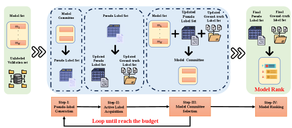
In this work, we propose LEMR (Label-Efficient Model Ranking), a framework that significantly reduces the need for costly annotations. Our framework operates without presuming the availability of ground-truth clean labels. Instead, we aim to strategically annotate instances from an unlabeled validation set for model ranking. The framework can be divided into four steps. First, an ensemble method with a selected model committee generates pseudo-labels for examples from the validation set, reducing the labeling cost (Step-I in Section 4.1). Subsequently, we address the inherent noise in these pseudo-labels through two strategies: We first use uncertainty sampling to acquire ground-truth labels (Step-II in Section 4.2)., and then utilize a Z-score mechanism to dynamically adjust the model committee based on these updated labels, further refining the labeling process (Step-III in Section 4.3). Finally, LEMR ranks all models using the refined pseudo-label and ground-truth label sets (Step-IV in Section 4.4). This framework allows us to create a design space for model ranking, facilitating a systematic exploration of the efficacy across different selection metrics and identifying optimal strategies for each stage.
Specifically, we first organize the intersection for our framework LEMR by proposing an explicit design space centered around disentangling the following key methodological considerations:
- •
-
•
Label Acquiring (Section 4.2): Which of the pseudo-labels needs to be acquired? Given the presence of noise in pseudo-labels, acquiring ground-truth labels is sometimes necessary. We employ uncertainty sampling strategies to identify which pseudo-labels to replace. Our approach includes uncertainty, classification margin, entropy, and random sampling strategies.
-
•
Model Committee Selection (Section 4.3): How to select a model committee reasonably? Selecting an appropriate model committee is crucial. We propose two methods: Z-score and All-model. The choice between them depends on balancing the desire for precision (favoring the Z-score method) and the need for diversity and comprehensive coverage (favoring the All-model approach).
With our design space, we can organize different methods and modularly generate a variety of methods. To evaluate these methods and facilitate future research in model ranking, we introduce the MoraBench (Model Ranking Benchmark) in Section 5. It covers diverse scenarios, including semi-supervised learning (Section 6.1), weak supervision (Section 6.2), and prompt selection (Section 6.3) tasks with 23 different tasks. The experiments on MoraBench lead to the following observations:
-
•
With a suitable combination of methods within the design space, our framework can dramatically reduce the labeling cost for model selection. For instance, in the semi-supervised learning scenario (AGNews task), labeling just 387 samples suffices for model selection, compared to the conventional need for 2000 samples.
-
•
In Pseudo-label Generation Step (Section 4.1), under a limited budget, we find that soft ensemble yields a higher quality model ranking if the model in the model set performs poorly, otherwise hard ensemble is a better choice.
-
•
In Active Label Acquisition Step (Section 4.2), our findings underline the superiority of uncertainty sampling over random acquisition in all tasks.
-
•
In Model Committee Selection Step (Section 4.3), We observe that a high-quality committee crucially influences the quality of model ranking. For this reason, a Z-score-based selection method is designed, which outperforms the All-model strategy on all datasets.
2 Related Work
2.1 Pseudo-labeling
Lately, pseudo-labeling has marked a significant progression in deep learning, utilizing models to predict unlabeled data samples Lee et al. (2013); Chen et al. (2021); Xu et al. (2023); Yang et al. (2023a); Zhang et al. (2022a). Zhu et al. (2023) explore self-adaptive pseudo-label filtering, aiming to refine the selection process for pseudo-labels to boost learning performance. Another popular technique is ensemble distillation Bachman et al. (2014); Hinton et al. (2015); Hu et al. (2023), which means distilling knowledge in an ensemble into a single model.
2.2 Model Selection
Model selection Kohavi (1995); Kayali and Wang (2022); Zhang et al. (2023) refers to determining the best from a set of candidate models based on their performance on a given dataset. In the domain of this area, current research encompasses a variety of innovative methodologies, especially in the field of natural language processing Yang et al. (2023b); Han et al. (2023); Du et al. (2021). Lu et al. (2022) leverage the entropy statistics to select the best prompt orders for in-context learning. Zhou et al. (2022) propose an unsupervised model selection criterion that encourages consistency but simultaneously penalizes collapse.
3 Preliminaries
In this work, we consider a -way classification task . For task , there exists trained models, denoted as . Our objective is to rank these models so that top-ranked models will achieve better performance on . Importantly, we work under the constraint of having no access to the original training data, instead relying on an unlabeled validation set , along with a limited annotation budget .
Our primary goal is to optimize the annotation process for the validation set in the context of model selection. To this end, we systematically study the effectiveness of our framework across different selection metrics and determine the optimal methods and timing for its utilization.
4 Methodology
To rank the trained models, we propose a novel framework LEMR, which comprises four primary steps. Step-I (Pseudo-label generation, Section 4.1): Generate pseudo-labels for the unlabeled validation set based on a model committee selected from the model set . Step-II (Active label acquisition, Section 4.2): Select samples from the validation set and acquires their ground-truth labels to replace the pseudo-labels. Step-III (Model committee selection, Section 4.3): Select a subset of models based on the updated pseudo-label to form a model committee that would be used to generate pseudo-labels in the next iteration. After rounds of iteration for these three steps, we obtain our final pseudo labels, based on which we perform our Step-IV (Model Ranking, Section 4.4). These four steps are detailed in Figure 1 and the pseudocode of LEMR is shown in Appendix A.
4.1 Step-I: Pseudo-label Generation
Our first step is to generate pseudo-labels based on a subset of trained models referred to as the model committee, which will be introduced soon. As the trained models usually have a certain level of capability on the task, it is natural to leverage their ensemble to obtain reasonable pseudo-labels Krogh and Vedelsby (1994); Hansen and Salamon (1990). In particular, we denote as the model committee at -th iteration, and explore two design choices of pseudo-label generation:
-
•
Hard ensemble: For , hard ensemble uses the average of the one-hot label prediction vectors generated by all models in as its pseudo-label distribution .
-
•
Soft ensemble: For , soft ensemble employs the average of the label probability simplex generated by all models in as its pseudo-label distribution .
Therefore, at -th iteration, we generate the pseudo-label for the -th sample via:
| (1) |
where the function could be either hard or soft ensemble. These pseudo-labels will be used to select high-quality models to form the model committee.
4.2 Step-II: Active Label Acquisition
In the second step of the LEMR framework, we actively acquire labels for a subset of samples from the pseudo-label set. We explore several existing active sampling strategies in the literature:
- •
-
•
Uncertainty Culotta and McCallum (2005): We define the value of 1 minus probabilities of the top predicted class as the uncertainty value for a pseudo-label.
-
•
Margin Schröder et al. (2022): Here, we target pseudo-labels with the smallest margin between the probabilities of the top two predicted classes.
-
•
Entropy Holub et al. (2008): This strategy calculates the entropy for each pseudo-label. With higher entropy indicating higher information, we prioritize acquiring labels with the highest entropy values.
Utilizing these strategies, we produce a set of samples at each iteration :
| (2) |
where represents a certain acquiring strategy (Uncertainty, Margin, Entropy, or Random) and is the current set of pseudo-labels. We then acquire ground-truth labels for the selected set .
We denote the set consisting of all ground-truth labels we have acquired as . For each sample in , we add its ground-truth label to and remove the corresponding pseudo-label from . This enhances the reliability of our pseudo-labels and refines subsequent steps, such as model committee selections.
4.3 Step-III: Model Committee Selection
The process of Model Committee Selection in our LEMR framework is a critical step to ensure the appropriate models are chosen to produce pseudo-labels for the next iteration. In our framework, we explore two distinct methods for model committee selection: Z-score and All-model:
-
•
All-model: All-model approach involves utilizing every model in the existing set as part of the model committee. It operates on the principle that the ensemble of diverse models can lead to a more generalized and comprehensive understanding, contributing to the robustness of the pseudo-labels generated.
-
•
Z-score: The Z-score method assesses a model’s performance relative to the median performance of the entire model set , aiding in the identification and filtering of outlier models with extremely low performance. It starts by calculating the accuracy of the -th model against the latest pseudo label set and ground-truth label set . Then, we calculate the Z-score for each model. Specifically, the Z-score of the model is determined as follows:
(3) where is the median of the . Subsequently, models with Z-score exceeding a certain threshold, , are selected for the next iteration’s committee. This ensures that only the most predictive and reliable models contribute to the pseudo-label generation.
Therefore, at the end of -th iteration, we select the model committee for the -th iteration as:
| (4) |
where the function could be either Z-score or All-model. Notably, with the updates of and , each time we choose the model committee from all models, not from the last model committee. This prevents the early exclusion of potentially valuable models, ensuring a robust and dynamic selection process throughout the iterations.
| Method | Dataset | ||||||||||||||||||||||
| Pseudo-label Generation | Active Label Acquisition | Model Committee Selection | IMDB (20) | AGNews (40) | Amazon Review (250) | Yelp Review (250) | Yahoo! Answer (500) | Avg. | |||||||||||||||
| 0% | 10% | 20% | 50% | 0% | 10% | 20% | 50% | 0% | 10% | 20% | 50% | 0% | 10% | 20% | 50% | 0% | 10% | 20% | 50% | ||||
| Hard Ensemble | Random | All-model | 0.98 | 0.97 | 1.09 | 0.76 | 5.38 | 5.35 | 5.31 | 0.69 | 9.47 | 9.50 | 9.48 | 9.47 | 14.27 | 14.27 | 14.27 | 0.62 | 7.11 | 7.01 | 6.82 | 0.93 | 6.19 |
| Z-score | 0.98 | 0.97 | 1.09 | 0.76 | 5.38 | 5.35 | 5.31 | 0.69 | 9.47 | 9.50 | 9.48 | 9.47 | 14.27 | 14.27 | 14.27 | 0.62 | 7.11 | 7.01 | 6.82 | 0.93 | 6.19 | ||
| Uncertainty | All-model | 0.98 | 0.84 | 0.77 | 0.12 | 5.38 | 4.81 | 0.21 | 0.01 | 9.47 | 9.48 | 9.54 | 6.90 | 14.27 | 14.27 | 14.28 | 0.44 | 7.11 | 6.37 | 1.06 | 0.02 | 5.32 | |
| Z-score | 0.98 | 0.24 | 0.00 | 0.00 | 5.38 | 4.41 | 0.24 | 0.01 | 9.47 | 9.45 | 9.38 | 5.66 | 14.27 | 14.30 | 14.28 | 0.60 | 7.11 | 6.36 | 0.99 | 0.04 | 5.16 | ||
| Margin | All-model | 0.98 | 0.84 | 0.77 | 0.12 | 5.38 | 4.79 | 0.23 | 0.01 | 9.47 | 9.50 | 9.56 | 7.34 | 14.27 | 14.27 | 14.28 | 0.45 | 7.11 | 6.69 | 1.13 | 0.03 | 5.36 | |
| Z-score | 0.98 | 0.24 | 0.00 | 0.00 | 5.38 | 4.57 | 0.22 | 0.01 | 9.47 | 9.45 | 9.38 | 6.52 | 14.27 | 14.31 | 14.26 | 0.59 | 7.11 | 6.56 | 1.24 | 0.02 | 5.23 | ||
| Entropy | All-model | 0.98 | 0.84 | 0.77 | 0.12 | 5.38 | 4.72 | 0.20 | 0.01 | 9.47 | 9.50 | 9.56 | 4.03 | 14.27 | 14.27 | 14.29 | 0.45 | 7.11 | 6.44 | 0.87 | 0.02 | 5.17 | |
| Z-score | 0.98 | 0.24 | 0.00 | 0.00 | 5.38 | 4.59 | 0.19 | 0.01 | 9.47 | 9.45 | 9.43 | 3.65 | 14.27 | 14.31 | 14.20 | 0.57 | 7.11 | 6.04 | 0.81 | 0.02 | 5.04 | ||
| Soft Ensemble | Random | All-model | 1.13 | 1.18 | 1.03 | 0.76 | 5.41 | 5.35 | 5.31 | 0.57 | 9.45 | 9.46 | 9.46 | 9.46 | 14.26 | 14.27 | 14.27 | 1.51 | 7.11 | 7.01 | 6.77 | 0.93 | 6.24 |
| Z-score | 1.13 | 1.18 | 1.03 | 0.76 | 5.41 | 5.35 | 5.31 | 0.57 | 9.45 | 9.46 | 9.46 | 9.46 | 14.26 | 14.27 | 14.27 | 1.51 | 7.11 | 7.01 | 6.77 | 0.93 | 6.24 | ||
| Uncertainty | All-model | 1.13 | 0.82 | 0.63 | 0.12 | 5.41 | 4.70 | 0.22 | 0.02 | 9.45 | 9.47 | 9.48 | 7.78 | 14.26 | 14.27 | 14.28 | 0.48 | 7.11 | 6.42 | 1.17 | 0.03 | 5.36 | |
| Z-score | 1.13 | 0.34 | 0.02 | 0.00 | 5.41 | 4.51 | 0.23 | 0.01 | 9.45 | 9.45 | 9.40 | 7.91 | 14.26 | 14.27 | 14.27 | 0.59 | 7.11 | 6.45 | 1.24 | 0.02 | 5.30 | ||
| Margin | All-model | 1.13 | 0.82 | 0.63 | 0.12 | 5.41 | 4.82 | 0.25 | 0.03 | 9.45 | 9.47 | 9.49 | 8.09 | 14.26 | 14.27 | 14.28 | 0.44 | 7.11 | 6.50 | 1.15 | 0.03 | 5.39 | |
| Z-score | 1.13 | 0.34 | 0.02 | 0.00 | 5.41 | 4.29 | 0.21 | 0.00 | 9.45 | 9.45 | 9.45 | 8.09 | 14.26 | 14.30 | 14.24 | 0.64 | 7.11 | 6.55 | 1.12 | 0.04 | 5.31 | ||
| Entropy | All-model | 1.13 | 0.82 | 0.63 | 0.12 | 5.41 | 4.61 | 0.20 | 0.03 | 9.45 | 9.45 | 9.49 | 7.10 | 14.26 | 14.27 | 14.27 | 0.51 | 7.11 | 6.31 | 0.97 | 0.00 | 5.31 | |
| Z-score | 1.13 | 0.34 | 0.02 | 0.00 | 5.41 | 4.59 | 0.17 | 0.01 | 9.45 | 9.45 | 9.45 | 7.15 | 14.26 | 14.31 | 14.28 | 0.64 | 7.11 | 6.30 | 0.94 | 0.03 | 5.25 | ||
| Method | Dataset | ||||||||||||||||||||||
| Pseudo-label Generation | Active Label Acquisition | Model Committee Selection | IMDB (100) | AGNews (200) | Amazon Review (1000) | Yelp Review (1000) | Yahoo! Answer (2000) | Avg. | |||||||||||||||
| 0% | 10% | 20% | 50% | 0% | 10% | 20% | 50% | 0% | 10% | 20% | 50% | 0% | 10% | 20% | 50% | 0% | 10% | 20% | 50% | ||||
| Hard Ensemble | Random | All-model | 0.96 | 0.96 | 0.91 | 0.86 | 4.85 | 4.90 | 4.85 | 2.17 | 7.25 | 7.24 | 7.23 | 7.20 | 8.64 | 8.65 | 8.65 | 7.33 | 5.83 | 5.77 | 5.71 | 0.70 | 5.03 |
| Z-score | 0.96 | 0.96 | 0.91 | 0.86 | 4.85 | 4.90 | 4.85 | 2.17 | 7.25 | 7.24 | 7.23 | 7.20 | 8.64 | 8.65 | 8.65 | 7.33 | 5.83 | 5.77 | 5.71 | 0.70 | 5.03 | ||
| Uncertainty | All-model | 0.96 | 0.66 | 0.65 | 0.06 | 4.85 | 4.28 | 0.05 | 0.01 | 7.25 | 7.17 | 7.14 | 2.60 | 8.64 | 8.63 | 8.66 | 0.36 | 5.83 | 5.39 | 0.70 | 0.01 | 3.70 | |
| Z-score | 0.96 | 0.67 | 0.04 | 0.00 | 4.85 | 4.47 | 0.04 | 0.00 | 7.25 | 7.24 | 7.03 | 2.70 | 8.64 | 8.71 | 8.67 | 0.34 | 5.83 | 5.26 | 0.66 | 0.01 | 3.67 | ||
| Margin | All-model | 0.96 | 0.66 | 0.65 | 0.06 | 4.85 | 4.48 | 0.07 | 0.01 | 7.25 | 7.19 | 7.10 | 2.62 | 8.64 | 8.65 | 8.70 | 0.39 | 5.83 | 5.24 | 0.87 | 0.00 | 3.71 | |
| Z-score | 0.96 | 0.67 | 0.04 | 0.00 | 4.85 | 4.44 | 0.05 | 0.00 | 7.25 | 7.26 | 7.17 | 2.83 | 8.64 | 8.69 | 8.69 | 0.31 | 5.83 | 5.21 | 0.85 | 0.00 | 3.69 | ||
| Entropy | All-model | 0.96 | 0.66 | 0.65 | 0.06 | 4.85 | 3.92 | 0.04 | 0.01 | 7.25 | 7.18 | 7.04 | 1.86 | 8.64 | 8.65 | 8.67 | 0.42 | 5.83 | 5.40 | 0.60 | 0.01 | 3.63 | |
| Z-score | 0.96 | 0.67 | 0.04 | 0.00 | 4.85 | 3.92 | 0.04 | 0.00 | 7.25 | 7.26 | 7.08 | 2.37 | 8.64 | 8.70 | 8.64 | 0.34 | 5.83 | 5.30 | 0.60 | 0.01 | 3.63 | ||
| Soft Ensemble | Random | All-model | 0.99 | 0.94 | 0.95 | 0.91 | 4.88 | 4.87 | 4.88 | 2.29 | 7.25 | 7.25 | 7.25 | 7.24 | 8.68 | 8.69 | 8.67 | 8.16 | 5.83 | 5.82 | 5.67 | 0.66 | 5.09 |
| Z-score | 0.99 | 0.94 | 0.95 | 0.91 | 4.88 | 4.87 | 4.88 | 2.29 | 7.25 | 7.25 | 7.25 | 7.24 | 8.68 | 8.69 | 8.67 | 8.16 | 5.83 | 5.82 | 5.67 | 0.66 | 5.09 | ||
| Uncertainty | All-model | 0.99 | 0.68 | 0.60 | 0.08 | 4.88 | 4.37 | 0.05 | 0.01 | 7.25 | 7.18 | 7.12 | 4.74 | 8.68 | 8.66 | 8.67 | 0.36 | 5.83 | 5.41 | 0.86 | 0.01 | 3.82 | |
| Z-score | 0.99 | 0.67 | 0.16 | 0.00 | 4.88 | 4.39 | 0.05 | 0.02 | 7.25 | 7.25 | 7.12 | 4.72 | 8.68 | 8.69 | 8.70 | 0.31 | 5.83 | 5.42 | 0.86 | 0.01 | 3.80 | ||
| Margin | All-model | 0.99 | 0.68 | 0.60 | 0.08 | 4.88 | 4.52 | 0.05 | 0.00 | 7.25 | 7.23 | 7.16 | 5.28 | 8.68 | 8.67 | 8.69 | 0.35 | 5.83 | 5.29 | 0.90 | 0.00 | 3.86 | |
| Z-score | 0.99 | 0.67 | 0.16 | 0.00 | 4.88 | 4.47 | 0.04 | 0.02 | 7.25 | 7.24 | 7.18 | 5.11 | 8.68 | 8.70 | 8.73 | 0.29 | 5.83 | 5.29 | 0.98 | 0.01 | 3.83 | ||
| Entropy | All-model | 0.99 | 0.68 | 0.60 | 0.08 | 4.88 | 4.30 | 0.05 | 0.01 | 7.25 | 7.18 | 7.13 | 4.85 | 8.68 | 8.66 | 8.64 | 0.41 | 5.83 | 5.54 | 0.61 | 0.00 | 3.82 | |
| Z-score | 0.99 | 0.67 | 0.16 | 0.00 | 4.88 | 4.35 | 0.03 | 0.02 | 7.25 | 7.19 | 7.15 | 4.55 | 8.68 | 8.72 | 8.70 | 0.35 | 5.83 | 5.56 | 0.58 | 0.00 | 3.78 | ||
| Method | Dataset | ||||||||||||
|---|---|---|---|---|---|---|---|---|---|---|---|---|---|
| Pseudo-label Generation | Active Label Acquisition | Model Committee Selection | IMDB | AGNews | Amazon Review | Yelp Review | Yahoo! Answer | Avg. | |||||
| 20 | 100 | 40 | 200 | 250 | 1000 | 250 | 1000 | 500 | 2000 | ||||
| Hard Ensemble | Random | All-model | 396 | 399 | 1442 | 1321 | 4230 | 4511 | 4363 | 3740 | 6865 | 7806 | 3507.7 |
| Z-score | 396 | 399 | 1442 | 1321 | 4230 | 4511 | 4363 | 3740 | 6865 | 7806 | 3507.7 | ||
| Uncertainty | All-model | 239 | 277 | 672 | 393 | 3984 | 3495 | 3959 | 3285 | 3304 | 3829 | 2344.1 | |
| Z-score | 57 | 97 | 668 | 392 | 3896 | 3355 | 3941 | 3107 | 3301 | 3829 | 2264.7 | ||
| Margin | All-model | 239 | 277 | 667 | 396 | 4057 | 3385 | 4137 | 3349 | 3336 | 3819 | 2366.8 | |
| Z-score | 57 | 97 | 671 | 391 | 3914 | 3369 | 3954 | 3124 | 3326 | 3879 | 2278.4 | ||
| Entropy | All-model | 239 | 277 | 668 | 387 | 3969 | 3586 | 3902 | 3382 | 3194 | 3813 | 2342.1 | |
| Z-score | 57 | 97 | 665 | 393 | 3881 | 3318 | 3919 | 3202 | 2959 | 3906 | 2240.0 | ||
| Soft Ensemble | Random | All-model | 396 | 399 | 1392 | 1291 | 4236 | 4523 | 4394 | 3860 | 7306 | 7805 | 3560.5 |
| Z-score | 396 | 399 | 1392 | 1291 | 4236 | 4523 | 4394 | 3860 | 7306 | 7805 | 3560.5 | ||
| Uncertainty | All-model | 219 | 277 | 709 | 395 | 4078 | 3546 | 3964 | 3369 | 3342 | 3950 | 2385.3 | |
| Z-score | 89 | 99 | 650 | 395 | 4026 | 3486 | 3961 | 3247 | 3320 | 3970 | 2324.6 | ||
| Margin | All-model | 219 | 277 | 692 | 394 | 4110 | 3511 | 4152 | 3364 | 3397 | 3902 | 2402.1 | |
| Z-score | 89 | 99 | 669 | 393 | 3968 | 3652 | 3979 | 3249 | 3364 | 3907 | 2337.2 | ||
| Entropy | All-model | 219 | 277 | 683 | 395 | 4006 | 3448 | 3952 | 3422 | 3272 | 3907 | 2358.6 | |
| Z-score | 89 | 99 | 673 | 394 | 3943 | 3604 | 3924 | 3272 | 3261 | 3975 | 2323.8 | ||
| Size of Unlabeled Validation Set | 400 | 400 | 2000 | 2000 | 5000 | 5000 | 5000 | 5000 | 10000 | 10000 | - | ||

| Method | Dataset | ||||||||||||||||||||||
| Pseudo-label Generation | Active Label Acquisition | Model Committee Selection | Yelp | SMS | IMDB | AGNews | Trec | Avg. | |||||||||||||||
| 0% | 10% | 20% | 50% | 0% | 10% | 20% | 50% | 0% | 10% | 20% | 50% | 0% | 10% | 20% | 50% | 0% | 10% | 20% | 50% | ||||
| Hard Ensemble | Random | All-model | 22.27 | 21.50 | 20.56 | 13.50 | 0.49 | 0.52 | 0.39 | 0.29 | 14.55 | 14.12 | 14.07 | 11.23 | 1.76 | 1.73 | 1.50 | 0.22 | 8.49 | 8.02 | 6.91 | 2.99 | 8.25 |
| Z-score | 22.27 | 21.50 | 20.56 | 13.50 | 0.49 | 0.52 | 0.39 | 0.29 | 14.55 | 14.12 | 14.07 | 11.23 | 1.76 | 1.73 | 1.50 | 0.22 | 8.49 | 8.02 | 6.91 | 2.99 | 8.25 | ||
| Uncertainty | All-model | 22.27 | 18.75 | 14.67 | 0.04 | 0.49 | 0.00 | 0.00 | 0.00 | 14.55 | 10.74 | 5.64 | 1.26 | 1.76 | 0.14 | 0.11 | 0.00 | 8.49 | 5.01 | 4.18 | 1.24 | 5.47 | |
| Z-score | 22.27 | 17.64 | 12.75 | 0.20 | 0.49 | 0.00 | 0.00 | 0.00 | 14.55 | 11.22 | 5.43 | 0.51 | 1.76 | 0.13 | 0.10 | 0.00 | 8.49 | 4.63 | 2.94 | 0.52 | 5.18 | ||
| Margin | All-model | 22.27 | 18.75 | 14.67 | 0.04 | 0.49 | 0.00 | 0.00 | 0.00 | 14.55 | 10.74 | 5.64 | 1.26 | 1.76 | 0.13 | 0.04 | 0.00 | 8.49 | 5.01 | 4.15 | 1.01 | 5.45 | |
| Z-score | 22.27 | 17.64 | 12.75 | 0.20 | 0.49 | 0.00 | 0.00 | 0.00 | 14.55 | 11.22 | 5.43 | 0.51 | 1.76 | 0.13 | 0.08 | 0.00 | 8.49 | 4.38 | 2.89 | 0.32 | 5.16 | ||
| Entropy | All-model | 22.27 | 18.75 | 14.67 | 0.04 | 0.49 | 0.00 | 0.00 | 0.00 | 14.55 | 10.74 | 5.64 | 1.26 | 1.76 | 0.04 | 0.12 | 0.00 | 8.49 | 5.62 | 4.68 | 1.20 | 5.52 | |
| Z-score | 22.27 | 17.64 | 12.75 | 0.20 | 0.49 | 0.00 | 0.00 | 0.00 | 14.55 | 11.22 | 5.43 | 0.51 | 1.76 | 0.09 | 0.14 | 0.00 | 8.49 | 4.90 | 3.17 | 0.66 | 5.21 | ||
| Soft Ensemble | Random | All-model | 22.16 | 21.17 | 20.09 | 13.30 | 0.49 | 0.52 | 0.39 | 0.29 | 14.19 | 13.67 | 13.54 | 11.33 | 1.76 | 1.74 | 1.53 | 0.24 | 8.86 | 8.69 | 7.79 | 3.61 | 8.27 |
| Z-score | 22.16 | 21.17 | 20.09 | 13.30 | 0.49 | 0.52 | 0.39 | 0.29 | 14.19 | 13.67 | 13.54 | 11.33 | 1.76 | 1.74 | 1.53 | 0.24 | 8.86 | 8.69 | 7.79 | 3.61 | 8.27 | ||
| Uncertainty | All-model | 22.16 | 18.24 | 13.69 | 0.41 | 0.49 | 0.01 | 0.00 | 0.00 | 14.19 | 10.21 | 5.53 | 0.25 | 1.76 | 0.14 | 0.14 | 0.00 | 8.86 | 4.98 | 4.10 | 0.87 | 5.30 | |
| Z-score | 22.16 | 16.89 | 12.96 | 0.07 | 0.49 | 0.01 | 0.00 | 0.00 | 14.19 | 10.76 | 6.44 | 0.63 | 1.76 | 0.14 | 0.14 | 0.00 | 8.86 | 4.77 | 3.63 | 0.85 | 5.24 | ||
| Margin | All-model | 22.16 | 18.24 | 13.69 | 0.41 | 0.49 | 0.01 | 0.00 | 0.00 | 14.19 | 10.21 | 5.53 | 0.25 | 1.76 | 0.05 | 0.14 | 0.00 | 8.86 | 4.97 | 3.35 | 1.18 | 5.27 | |
| Z-score | 22.16 | 16.89 | 12.96 | 0.07 | 0.49 | 0.01 | 0.00 | 0.00 | 14.19 | 10.76 | 6.44 | 0.63 | 1.76 | 0.05 | 0.14 | 0.00 | 8.86 | 4.77 | 2.90 | 0.97 | 5.20 | ||
| Entropy | All-model | 22.16 | 18.24 | 13.69 | 0.41 | 0.49 | 0.01 | 0.00 | 0.00 | 14.19 | 10.21 | 5.53 | 0.25 | 1.76 | 0.06 | 0.10 | 0.00 | 8.86 | 6.04 | 4.50 | 1.07 | 5.38 | |
| Z-score | 22.16 | 16.89 | 12.96 | 0.07 | 0.49 | 0.01 | 0.00 | 0.00 | 14.19 | 10.76 | 6.44 | 0.63 | 1.76 | 0.10 | 0.14 | 0.00 | 8.86 | 5.00 | 3.73 | 0.83 | 5.25 | ||

| Method | Dataset | ||||||||||||||||||||||||||
| Pseudo-label Generation | Active Label Acquisition | Model Committee Selection | WSC | Story | CB | RTE | WiC | ANLI1 | ANLI2 | ANLI3 | Avg. | ||||||||||||||||
| 0% | 10% | 30% | 0% | 10% | 30% | 0% | 10% | 30% | 0% | 10% | 30% | 0% | 10% | 30% | 0% | 10% | 30% | 0% | 10% | 30% | 0% | 10% | 30% | ||||
| Hard Ensemble | Random | All Model | 1.16 | 0.95 | 1.04 | 0.03 | 0.02 | 0.01 | 2.84 | 2.67 | 1.82 | 0.40 | 0.38 | 0.50 | 1.14 | 0.86 | 0.82 | 0.05 | 0.06 | 0.06 | 0.46 | 0.48 | 0.40 | 0.81 | 0.80 | 0.82 | 0.77 |
| Z-score | 1.16 | 0.95 | 1.04 | 0.03 | 0.02 | 0.01 | 2.84 | 2.67 | 1.82 | 0.40 | 0.38 | 0.50 | 1.14 | 0.86 | 0.82 | 0.05 | 0.06 | 0.06 | 0.46 | 0.48 | 0.40 | 0.81 | 0.80 | 0.82 | 0.77 | ||
| Uncertainty | All Model | 1.16 | 0.64 | 0.03 | 0.03 | 0.03 | 0.01 | 2.84 | 1.60 | 0.40 | 0.40 | 0.07 | 0.40 | 1.14 | 1.05 | 0.04 | 0.05 | 0.07 | 0.46 | 0.46 | 0.33 | 0.44 | 0.81 | 0.86 | 0.85 | 0.59 | |
| Z-score | 1.16 | 0.00 | 0.03 | 0.03 | 0.00 | 0.00 | 2.84 | 0.00 | 0.00 | 0.40 | 0.00 | 0.00 | 1.14 | 1.19 | 0.17 | 0.05 | 0.13 | 0.57 | 0.46 | 0.26 | 0.45 | 0.81 | 0.81 | 0.83 | 0.47 | ||
| Margin | All Model | 1.16 | 0.64 | 0.03 | 0.03 | 0.03 | 0.01 | 2.84 | 1.64 | 0.27 | 0.40 | 0.07 | 0.40 | 1.14 | 1.05 | 0.04 | 0.05 | 0.23 | 0.55 | 0.46 | 0.33 | 0.49 | 0.81 | 0.94 | 0.85 | 0.60 | |
| Z-score | 1.16 | 0.00 | 0.03 | 0.03 | 0.00 | 0.00 | 2.84 | 0.00 | 0.00 | 0.40 | 0.00 | 0.00 | 1.14 | 1.19 | 0.17 | 0.05 | 0.11 | 0.51 | 0.46 | 0.27 | 0.42 | 0.81 | 0.77 | 0.75 | 0.46 | ||
| Entropy | All Model | 1.16 | 0.64 | 0.03 | 0.03 | 0.03 | 0.01 | 2.84 | 1.42 | 0.31 | 0.40 | 0.07 | 0.40 | 1.14 | 1.05 | 0.04 | 0.05 | 0.10 | 0.51 | 0.46 | 0.31 | 0.45 | 0.81 | 0.66 | 0.85 | 0.57 | |
| Z-score | 1.16 | 0.00 | 0.03 | 0.03 | 0.00 | 0.00 | 2.84 | 0.00 | 0.00 | 0.40 | 0.00 | 0.00 | 1.14 | 1.19 | 0.17 | 0.05 | 0.08 | 0.56 | 0.46 | 0.31 | 0.43 | 0.81 | 0.83 | 0.76 | 0.47 | ||
| Soft Ensemble | Random | All Model | 2.12 | 2.01 | 1.33 | 0.04 | 0.04 | 0.02 | 2.84 | 2.71 | 1.91 | 1.40 | 1.33 | 1.02 | 0.19 | 0.10 | 0.16 | 0.20 | 0.22 | 0.08 | 0.55 | 0.54 | 0.57 | 1.18 | 1.17 | 1.13 | 0.95 |
| Z-score | 2.12 | 2.01 | 1.33 | 0.04 | 0.04 | 0.02 | 2.84 | 2.71 | 1.91 | 1.40 | 1.33 | 1.02 | 0.19 | 0.10 | 0.16 | 0.20 | 0.22 | 0.08 | 0.55 | 0.54 | 0.57 | 1.18 | 1.17 | 1.13 | 0.95 | ||
| Uncertainty | All Model | 2.12 | 1.10 | 0.04 | 0.04 | 0.01 | 0.00 | 2.84 | 1.29 | 0.36 | 1.40 | 2.64 | 2.00 | 0.19 | 0.52 | 0.14 | 0.20 | 0.22 | 0.58 | 0.55 | 0.44 | 0.37 | 1.18 | 0.99 | 0.80 | 0.83 | |
| Z-score | 2.12 | 0.00 | 0.04 | 0.04 | 0.00 | 0.00 | 2.84 | 0.00 | 0.00 | 1.40 | 0.00 | 0.00 | 0.19 | 0.77 | 0.16 | 0.20 | 0.20 | 0.43 | 0.55 | 0.47 | 0.33 | 1.18 | 0.88 | 0.97 | 0.53 | ||
| Margin | All Model | 2.12 | 1.10 | 0.04 | 0.04 | 0.01 | 0.00 | 2.84 | 1.20 | 0.04 | 1.40 | 2.64 | 2.00 | 0.19 | 0.52 | 0.14 | 0.20 | 0.36 | 0.55 | 0.55 | 0.50 | 0.31 | 1.18 | 1.07 | 0.90 | 0.83 | |
| Z-score | 2.12 | 0.00 | 0.04 | 0.04 | 0.00 | 0.00 | 2.84 | 0.00 | 0.00 | 1.40 | 0.00 | 0.00 | 0.19 | 0.77 | 0.16 | 0.20 | 0.32 | 0.56 | 0.55 | 0.48 | 0.41 | 1.18 | 1.04 | 0.91 | 0.55 | ||
| Entropy | All Model | 2.12 | 1.10 | 0.04 | 0.04 | 0.01 | 0.00 | 2.84 | 1.42 | 1.07 | 1.40 | 2.64 | 2.00 | 0.19 | 0.52 | 0.14 | 0.20 | 0.03 | 0.30 | 0.55 | 0.44 | 0.59 | 1.18 | 0.94 | 1.02 | 0.87 | |
| Z-score | 2.12 | 0.00 | 0.04 | 0.04 | 0.00 | 0.00 | 2.84 | 0.00 | 0.00 | 1.40 | 0.00 | 0.00 | 0.19 | 0.77 | 0.16 | 0.20 | 0.02 | 0.27 | 0.55 | 0.44 | 0.27 | 1.18 | 0.81 | 1.07 | 0.52 | ||

4.4 Step-IV: Model Ranking
Step-IV in the LEMR framework is dedicated to ranking the models in the set . This step utilizes the final pseudo-label set and the ground-truth label set to evaluate each model’s accuracy. The rank is determined as:
| (5) |
where is the ranking function. It ranks the models in according to their accuracy on and .
5 The MoraBench Benchmark
To advance research in model ranking and evaluate various design choices in our LEMR framework, we introduce MoraBench (Model Ranking Benchmark). This benchmark comprises a collection of model outputs generated under diverse scenarios. The description of all model sets within MoraBench and its generation configuration are given in Appendix C. We then perform model selection based on these outputs. MoraBench and its associated resources are available at http://github.com/ppsmk388/MoraBench.
5.1 Evaluation Metrics
We define two metrics used to evaluate the effectiveness of model selection results, namely Optimal Gap and Ranking Correction.
Optimal Gap.
The Optimal Gap is defined as the difference in test accuracy between the best model chosen by the fully-labeled validation set, and the best model identified by the methods to be assessed.
Ranking Correction.
Ranking Correction measures the similarity between the model rankings based on the fully-labeled validation set and those obtained by methods to be assessed. This similarity is assessed using the Spearman rank correlation coefficient111http://docs.scipy.org/doc/scipy/reference/generated/scipy.stats.spearmanr.html , a common non-parametric method evaluating the monotonic relationship between two ranked variables.
6 Experiments
We test our LEMR with MoraBench in detail under three scenarios, i.e., semi-supervised learning (Section 6.1), weak supervision (Section 6.2), and prompt selection (Section 6.3). Corresponding implementation details and design space are described in Appendix B.
6.1 Semi-supervised Learning Setting
Here, we evaluate the LEMR framework under a semi-supervised learning setting. For clarity, we first introduce the concept of ’budget ratio’, defined as the proportion of our budget relative to the size of the complete unlabeled validation set. We examined the performance of LEMR at different budget ratios (0%, 10%, 20% and 50%), and relevant results are detailed in Tables 1 and 2. The impact of varying budget ratios on ranking correction is shown in Figure 2. Additionally, Table 3 highlights the minimum budget needed to achieve an optimal gap of 0. The number in brackets after the dataset indicates the number of labels used in the model training stage. The model set generation setups can be found in Appendix C.1.
From the results, we have the following findings: First, LEMR significantly minimizes labeling costs for model selection. For instance, in setting AGNews (200), we only need to label 387 samples to select the same model as labeling the entire validation set of 2000 samples (see Table 3). Second, our results consistently show the superiority of uncertainty sampling over random sampling. Table 3 illustrates that random sampling typically requires a significantly larger budget compared to uncertainty sampling. This trend is evident in Table 1 and Table 2 as well. Additionally, the curves representing the random strategy in Figure 2 consistently lie below of other uncertainty sampling strategies. Finally, the model committee selected by Z-score is better than All-model under our design space. For example, in Table 1 and 2, the Z-score has a smaller optimal gap than All-model in all cases.
6.2 Weak Supervision Setting
In this section, we employed the WRENCH Zhang et al. (2021b) to evaluate our LEMR framework within a weak supervision setting. we first evaluate LEMR in a low-budget setting. Specifically, we test our framework with budget ratios of 0%, 10%, 20%, and 50%. The corresponding optimal values are displayed in Table 4. Additionally, Figure 2 illustrates the variation in ranking correction as the budget ratio increases from 0 to 1. The model set generation setups can be found in Appendix C.2. Some interesting observations are shown as follows: First, LEMR, when combined with an appropriate selection of methods, significantly lowers the labeling cost for validation sets: As shown in Table 4, only 10% of the labeling cost suffices to select the same model that would be chosen with a fully labeled validation set. Then, compared to random sampling, uncertainty sampling strategies consistently exhibit superior performance. This is evident in Table 4, where the optimal gap for random sampling is highest across all budgets. Moreover, from Figure 2, we notice the random strategy has a curve below all uncertainty sampling strategies, which further supports our conclusion. Finally, adopting the Z-score method generally reduces labeling costs as evidenced by the lower optimal gap values in Table 4. This suggests that removing the model that contains noise helps to reduce the labeling cost.
6.3 Prompt Selection Setting
In this section, we employ the T0 benchmark Sanh et al. (2022) to test LEMR under the prompt selection task. With a large language model, denoted as , and a set of prompts , we can analogize to and refer to Step-I (Section 4.1) to Step-IV (Section 4.4) to get the model rank. The experimental results, including the optimal gap for budget ratios of 0%, 10%, and 30%, are summarized in Table 5. Additionally, Figure 4 visually represents the changes in ranking correction as budget ratios vary from 0 to 1. The setups for model set generation can be found in Appendix C.3.
First, in Figure 4, we find that under a limited budget, soft ensemble yields higher quality model rank if the model in the model set performs poorly, whereas hard ensemble is the superior solution. For example, in the low-budget case, hard ensemble is a better choice in tasks RTE, Story, and WSC, where models generally perform better. While in tasks WIC, ANL1, ANL2, and ANL3, where models perform worse, soft ensemble works better. A similar situation can be found in the Yelp (250), Amazon (100), Amazon (250), Yahoo (500), and Yahoo (2000) datasets in the semi-supervised setting (in Figure 2) as well as in the AGNews dataset and Trec dataset in the weakly supervised setting (in Figure 3). An intuitive explanation is that when the model’s performance in the model set is poor, soft ensemble can utilize all the model’s uncertainty information about the data, while hard ensemble may rely too much on some wrong prediction results, so soft ensemble will be more suitable in this case. When the model’s performance in the model set is relatively high, hard ensemble can filter out the noisy information, which is more conducive to obtaining a high quality rank. When the models in the model set all perform exceptionally well (SMS task of weak supervision setting in Figure 3) or when the model predictions in the model set are relatively consistent (CB tasks of prompt selection), the results of the hard ensemble and the soft ensemble will remain consistent. Moreover, our framework exhibits a substantial reduction in the labeling costs for validation sets. For example, as demonstrated in Table 5, for the SMS task, achieving an optimal gap value of 0 necessitates only 10% budget ratio. Besides, we find that when the sampling strategy is random, the optimal gap of the random strategy is the largest regardless of the budget ratio in Table 5. Lastly, we observe that using Z-score reduces the budget required for all tasks. On average, the Z-score method yields a lower optimal gap value in Table 5. This suggests that a high-quality committee can generate a high-quality model ranking.
7 Conclusion
In this paper, we introduce LEMR, a novel framework that significantly reduces labeling costs for model selection tasks, particularly under resource-limited settings. To evaluate LEMR, we propose the MoraBench Benchmark, a comprehensive collection of model outputs across diverse scenarios. Demonstrated across 23 tasks, including semi-supervised learning, weak supervision, and prompt selection, LEMR significantly reduces validation labeling costs without compromising accuracy. Key results show that, in certain tasks, the required labeling effort is reduced to below 10% compared to a fully labeled dataset. Our findings emphasize the importance of selecting suitable ensemble methods based on model performance, the superiority of uncertainty sampling over random strategies, and the importance of selecting suitable modes to compose the model committee.
References
- (1) "yelp dataset: http://www.yelp.com/dataset_challenge".
- Almeida et al. (2011) Tiago A Almeida, José María G Hidalgo, and Akebo Yamakami. 2011. Contributions to the study of sms spam filtering: new collection and results. In DocEng, pages 259–262.
- Awasthi et al. (2020) Abhijeet Awasthi, Sabyasachi Ghosh, Rasna Goyal, and Sunita Sarawagi. 2020. Learning from rules generalizing labeled exemplars. In 8th International Conference on Learning Representations, ICLR 2020, Addis Ababa, Ethiopia, April 26-30, 2020. OpenReview.net.
- Awasthy et al. (2020) Parul Awasthy, Bishwaranjan Bhattacharjee, John Kender, and Radu Florian. 2020. Predictive model selection for transfer learning in sequence labeling tasks. In Proceedings of SustaiNLP: Workshop on Simple and Efficient Natural Language Processing, pages 113–118, Online. Association for Computational Linguistics.
- Bach et al. (2017) Stephen H. Bach, Bryan Dawei He, Alexander Ratner, and Christopher Ré. 2017. Learning the structure of generative models without labeled data. In Proceedings of the 34th International Conference on Machine Learning, ICML 2017, Sydney, NSW, Australia, 6-11 August 2017, volume 70 of Proceedings of Machine Learning Research, pages 273–282. PMLR.
- Bachman et al. (2014) Philip Bachman, Ouais Alsharif, and Doina Precup. 2014. Learning with pseudo-ensembles. In Advances in Neural Information Processing Systems 27: Annual Conference on Neural Information Processing Systems 2014, December 8-13 2014, Montreal, Quebec, Canada, pages 3365–3373.
- Bergstra and Bengio (2012) James Bergstra and Yoshua Bengio. 2012. Random search for hyper-parameter optimization. Journal of machine learning research, 13(2).
- Berthelot et al. (2019a) David Berthelot, Nicholas Carlini, Ekin D Cubuk, Alex Kurakin, Kihyuk Sohn, Han Zhang, and Colin Raffel. 2019a. Remixmatch: Semi-supervised learning with distribution alignment and augmentation anchoring. ArXiv preprint, abs/1911.09785.
- Berthelot et al. (2019b) David Berthelot, Nicholas Carlini, Ian J. Goodfellow, Nicolas Papernot, Avital Oliver, and Colin Raffel. 2019b. Mixmatch: A holistic approach to semi-supervised learning. In Advances in Neural Information Processing Systems 32: Annual Conference on Neural Information Processing Systems 2019, NeurIPS 2019, December 8-14, 2019, Vancouver, BC, Canada, pages 5050–5060.
- Berthelot et al. (2022) David Berthelot, Rebecca Roelofs, Kihyuk Sohn, Nicholas Carlini, and Alexey Kurakin. 2022. Adamatch: A unified approach to semi-supervised learning and domain adaptation. In The Tenth International Conference on Learning Representations, ICLR 2022, Virtual Event, April 25-29, 2022. OpenReview.net.
- Blier and Ollivier (2018) Léonard Blier and Yann Ollivier. 2018. The description length of deep learning models. In Advances in Neural Information Processing Systems 31: Annual Conference on Neural Information Processing Systems 2018, NeurIPS 2018, December 3-8, 2018, Montréal, Canada, pages 2220–2230.
- Bragg et al. (2021) Jonathan Bragg, Arman Cohan, Kyle Lo, and Iz Beltagy. 2021. FLEX: unifying evaluation for few-shot NLP. In Advances in Neural Information Processing Systems 34: Annual Conference on Neural Information Processing Systems 2021, NeurIPS 2021, December 6-14, 2021, virtual, pages 15787–15800.
- Chang et al. (2008) Ming-Wei Chang, Lev-Arie Ratinov, Dan Roth, and Vivek Srikumar. 2008. Importance of semantic representation: Dataless classification. In Aaai, volume 2, pages 830–835.
- Chen et al. (2021) Yiming Chen, Yan Zhang, Chen Zhang, Grandee Lee, Ran Cheng, and Haizhou Li. 2021. Revisiting self-training for few-shot learning of language model. In Proceedings of the 2021 Conference on Empirical Methods in Natural Language Processing, pages 9125–9135, Online and Punta Cana, Dominican Republic. Association for Computational Linguistics.
- Choi et al. (2022) HongSeok Choi, Dongha Choi, and Hyunju Lee. 2022. Early stopping based on unlabeled samples in text classification. In Proceedings of the 60th Annual Meeting of the Association for Computational Linguistics (Volume 1: Long Papers), pages 708–718, Dublin, Ireland. Association for Computational Linguistics.
- Culotta and McCallum (2005) Aron Culotta and Andrew McCallum. 2005. Reducing labeling effort for structured prediction tasks. In AAAI, volume 5, pages 746–751.
- Dagan et al. (2006) Ido Dagan, Oren Glickman, and Bernardo Magnini. 2006. The pascal recognising textual entailment challenge. In Machine Learning Challenges. Evaluating Predictive Uncertainty, Visual Object Classification, and Recognising Tectual Entailment, pages 177–190, Berlin, Heidelberg. Springer Berlin Heidelberg.
- De Marneffe et al. (2019) Marie-Catherine De Marneffe, Mandy Simons, and Judith Tonhauser. 2019. The commitmentbank: Investigating projection in naturally occurring discourse. In proceedings of Sinn und Bedeutung, volume 23, pages 107–124.
- Du et al. (2021) Zhengxiao Du, Yujie Qian, Xiao Liu, Ming Ding, Jiezhong Qiu, Zhilin Yang, and Jie Tang. 2021. All nlp tasks are generation tasks: A general pretraining framework. ArXiv preprint, abs/2103.10360.
- Fan et al. (2021) Yue Fan, Anna Kukleva, and Bernt Schiele. 2021. Revisiting consistency regularization for semi-supervised learning. In DAGM German Conference on Pattern Recognition, pages 63–78. Springer.
- Han et al. (2023) Xudong Han, Timothy Baldwin, and Trevor Cohn. 2023. Fair enough: Standardizing evaluation and model selection for fairness research in NLP. In Proceedings of the 17th Conference of the European Chapter of the Association for Computational Linguistics, pages 297–312, Dubrovnik, Croatia. Association for Computational Linguistics.
- Hansen and Salamon (1990) Lars Kai Hansen and Peter Salamon. 1990. Neural network ensembles. IEEE transactions on pattern analysis and machine intelligence, 12(10):993–1001.
- Hinton et al. (2015) Geoffrey Hinton, Oriol Vinyals, and Jeff Dean. 2015. Distilling the knowledge in a neural network. ArXiv preprint, abs/1503.02531.
- Holub et al. (2008) Alex Holub, Pietro Perona, and Michael C. Burl. 2008. Entropy-based active learning for object recognition. In 2008 IEEE Computer Society Conference on Computer Vision and Pattern Recognition Workshops, pages 1–8.
- Hu et al. (2023) Zhengyu Hu, Jieyu Zhang, Haonan Wang, Siwei Liu, and Shangsong Liang. 2023. Leveraging relational graph neural network for transductive model ensemble. In Proceedings of the 29th ACM SIGKDD Conference on Knowledge Discovery and Data Mining, pages 775–787.
- Kayali and Wang (2022) Moe Kayali and Chi Wang. 2022. Mining robust default configurations for resource-constrained automl. ArXiv, abs/2202.09927.
- Kohavi (1995) Ron Kohavi. 1995. A study of cross-validation and bootstrap for accuracy estimation and model selection. In International Joint Conference on Artificial Intelligence.
- Krogh and Vedelsby (1994) Anders Krogh and Jesper Vedelsby. 1994. Neural network ensembles, cross validation, and active learning. Advances in neural information processing systems, 7.
- Lee et al. (2013) Dong-Hyun Lee et al. 2013. Pseudo-label: The simple and efficient semi-supervised learning method for deep neural networks. In Workshop on challenges in representation learning, ICML, volume 3, page 896. Atlanta.
- Levesque et al. (2012) Hector Levesque, Ernest Davis, and Leora Morgenstern. 2012. The winograd schema challenge. In Thirteenth International Conference on the Principles of Knowledge Representation and Reasoning. Citeseer.
- Li et al. (2021) Junnan Li, Caiming Xiong, and Steven C. H. Hoi. 2021. Comatch: Semi-supervised learning with contrastive graph regularization. In 2021 IEEE/CVF International Conference on Computer Vision, ICCV 2021, Montreal, QC, Canada, October 10-17, 2021, pages 9455–9464. IEEE.
- Li and Roth (2002) Xin Li and Dan Roth. 2002. Learning question classifiers. In International Conference on Computational Linguistics.
- Liu et al. (2022) Haokun Liu, Derek Tam, Muqeeth Mohammed, Jay Mohta, Tenghao Huang, Mohit Bansal, and Colin Raffel. 2022. Few-shot parameter-efficient fine-tuning is better and cheaper than in-context learning. In Advances in Neural Information Processing Systems.
- Liu and Wang (2021) Xueqing Liu and Chi Wang. 2021. An empirical study on hyperparameter optimization for fine-tuning pre-trained language models. In Proceedings of the 59th Annual Meeting of the Association for Computational Linguistics and the 11th International Joint Conference on Natural Language Processing (Volume 1: Long Papers), pages 2286–2300, Online. Association for Computational Linguistics.
- Lizotte (2021) Dan Lizotte. 2021. Model selection. Machine Learning — A Journey to Deep Learning.
- Lu et al. (2022) Yao Lu, Max Bartolo, Alastair Moore, Sebastian Riedel, and Pontus Stenetorp. 2022. Fantastically ordered prompts and where to find them: Overcoming few-shot prompt order sensitivity. In Proceedings of the 60th Annual Meeting of the Association for Computational Linguistics (Volume 1: Long Papers), pages 8086–8098, Dublin, Ireland. Association for Computational Linguistics.
- Maas et al. (2011) Andrew L. Maas, Raymond E. Daly, Peter T. Pham, Dan Huang, Andrew Y. Ng, and Christopher Potts. 2011. Learning word vectors for sentiment analysis. In Proceedings of the 49th Annual Meeting of the Association for Computational Linguistics: Human Language Technologies, pages 142–150, Portland, Oregon, USA. Association for Computational Linguistics.
- Mahsereci et al. (2017) Maren Mahsereci, Lukas Balles, Christoph Lassner, and Philipp Hennig. 2017. Early stopping without a validation set. ArXiv preprint, abs/1703.09580.
- McAuley and Leskovec (2013) Julian J. McAuley and Jure Leskovec. 2013. Hidden factors and hidden topics: understanding rating dimensions with review text. In Seventh ACM Conference on Recommender Systems, RecSys ’13, Hong Kong, China, October 12-16, 2013, pages 165–172. ACM.
- Miyato et al. (2018) Takeru Miyato, Shin-ichi Maeda, Masanori Koyama, and Shin Ishii. 2018. Virtual adversarial training: a regularization method for supervised and semi-supervised learning. IEEE transactions on pattern analysis and machine intelligence, 41(8):1979–1993.
- Mostafazadeh et al. (2017) Nasrin Mostafazadeh, Michael Roth, Annie Louis, Nathanael Chambers, and James Allen. 2017. LSDSem 2017 shared task: The story cloze test. In Proceedings of the 2nd Workshop on Linking Models of Lexical, Sentential and Discourse-level Semantics, pages 46–51, Valencia, Spain. Association for Computational Linguistics.
- Nie et al. (2020) Yixin Nie, Adina Williams, Emily Dinan, Mohit Bansal, Jason Weston, and Douwe Kiela. 2020. Adversarial NLI: A new benchmark for natural language understanding. In Proceedings of the 58th Annual Meeting of the Association for Computational Linguistics, pages 4885–4901, Online. Association for Computational Linguistics.
- OpenAI (2023) OpenAI. 2023. Gpt-4 technical report. ArXiv preprint, abs/2303.08774.
- Penrose (1946) Lionel S Penrose. 1946. The elementary statistics of majority voting. Journal of the Royal Statistical Society, 109(1):53–57.
- Perez et al. (2021) Ethan Perez, Douwe Kiela, and Kyunghyun Cho. 2021. True few-shot learning with language models. In Advances in Neural Information Processing Systems 34: Annual Conference on Neural Information Processing Systems 2021, NeurIPS 2021, December 6-14, 2021, virtual, pages 11054–11070.
- Pilehvar and Camacho-Collados (2019) Mohammad Taher Pilehvar and Jose Camacho-Collados. 2019. WiC: the word-in-context dataset for evaluating context-sensitive meaning representations. In Proceedings of the 2019 Conference of the North American Chapter of the Association for Computational Linguistics: Human Language Technologies, Volume 1 (Long and Short Papers), pages 1267–1273, Minneapolis, Minnesota. Association for Computational Linguistics.
- Rasmus et al. (2015) Antti Rasmus, Mathias Berglund, Mikko Honkala, Harri Valpola, and Tapani Raiko. 2015. Semi-supervised learning with ladder networks. In Advances in Neural Information Processing Systems 28: Annual Conference on Neural Information Processing Systems 2015, December 7-12, 2015, Montreal, Quebec, Canada, pages 3546–3554.
- Ratner et al. (2017) Alexander J. Ratner, Stephen H. Bach, Henry R. Ehrenberg, and Christopher Ré. 2017. Snorkel: Fast training set generation for information extraction. In Proceedings of the 2017 ACM International Conference on Management of Data, SIGMOD Conference 2017, Chicago, IL, USA, May 14-19, 2017, pages 1683–1686. ACM.
- Rawat et al. (2021) Ankit Singh Rawat, Aditya Krishna Menon, Wittawat Jitkrittum, Sadeep Jayasumana, Felix X. Yu, Sashank J. Reddi, and Sanjiv Kumar. 2021. Disentangling sampling and labeling bias for learning in large-output spaces. In Proceedings of the 38th International Conference on Machine Learning, ICML 2021, 18-24 July 2021, Virtual Event, volume 139 of Proceedings of Machine Learning Research, pages 8890–8901. PMLR.
- Ren et al. (2020) Wendi Ren, Yinghao Li, Hanting Su, David Kartchner, Cassie Mitchell, and Chao Zhang. 2020. Denoising multi-source weak supervision for neural text classification. In Findings of the Association for Computational Linguistics: EMNLP 2020, pages 3739–3754, Online. Association for Computational Linguistics.
- Sanh et al. (2022) Victor Sanh, Albert Webson, Colin Raffel, Stephen H. Bach, Lintang Sutawika, Zaid Alyafeai, Antoine Chaffin, Arnaud Stiegler, Arun Raja, Manan Dey, et al. 2022. Multitask prompted training enables zero-shot task generalization. In The Tenth International Conference on Learning Representations, ICLR 2022, Virtual Event, April 25-29, 2022. OpenReview.net.
- Schröder et al. (2022) Christopher Schröder, Andreas Niekler, and Martin Potthast. 2022. Revisiting uncertainty-based query strategies for active learning with transformers. In Findings of the Association for Computational Linguistics: ACL 2022, pages 2194–2203, Dublin, Ireland. Association for Computational Linguistics.
- Severyn and Moschitti (2013) Aliaksei Severyn and Alessandro Moschitti. 2013. Automatic feature engineering for answer selection and extraction. In Proceedings of the 2013 Conference on Empirical Methods in Natural Language Processing, pages 458–467, Seattle, Washington, USA. Association for Computational Linguistics.
- Sohn et al. (2020) Kihyuk Sohn, David Berthelot, Nicholas Carlini, Zizhao Zhang, Han Zhang, Colin Raffel, Ekin Dogus Cubuk, Alexey Kurakin, and Chun-Liang Li. 2020. Fixmatch: Simplifying semi-supervised learning with consistency and confidence. In Advances in Neural Information Processing Systems 33: Annual Conference on Neural Information Processing Systems 2020, NeurIPS 2020, December 6-12, 2020, virtual.
- Tarvainen and Valpola (2017) Antti Tarvainen and Harri Valpola. 2017. Mean teachers are better role models: Weight-averaged consistency targets improve semi-supervised deep learning results. In Advances in Neural Information Processing Systems 30: Annual Conference on Neural Information Processing Systems 2017, December 4-9, 2017, Long Beach, CA, USA, pages 1195–1204.
- Wang et al. (2022) Yidong Wang, Hao Chen, Yue Fan, Wang Sun, Ran Tao, Wenxin Hou, Renjie Wang, Linyi Yang, Zhi Zhou, Lan-Zhe Guo, et al. 2022. Usb: A unified semi-supervised learning benchmark for classification. Advances in Neural Information Processing Systems, 35:3938–3961.
- Xie et al. (2020) Qizhe Xie, Zihang Dai, Eduard H. Hovy, Thang Luong, and Quoc Le. 2020. Unsupervised data augmentation for consistency training. In Advances in Neural Information Processing Systems 33: Annual Conference on Neural Information Processing Systems 2020, NeurIPS 2020, December 6-12, 2020, virtual.
- Xu et al. (2023) Ran Xu, Yue Yu, Hejie Cui, Xuan Kan, Yanqiao Zhu, Joyce Ho, Chao Zhang, and Carl Yang. 2023. Neighborhood-regularized self-training for learning with few labels. ArXiv preprint, abs/2301.03726.
- Xu et al. (2021) Yi Xu, Lei Shang, Jinxing Ye, Qi Qian, Yu-Feng Li, Baigui Sun, Hao Li, and Rong Jin. 2021. Dash: Semi-supervised learning with dynamic thresholding. In Proceedings of the 38th International Conference on Machine Learning, ICML 2021, 18-24 July 2021, Virtual Event, volume 139 of Proceedings of Machine Learning Research, pages 11525–11536. PMLR.
- Yang et al. (2023a) Weiyi Yang, Richong Zhang, Junfan Chen, Lihong Wang, and Jaein Kim. 2023a. Prototype-guided pseudo labeling for semi-supervised text classification. In Proceedings of the 61st Annual Meeting of the Association for Computational Linguistics (Volume 1: Long Papers), pages 16369–16382, Toronto, Canada. Association for Computational Linguistics.
- Yang et al. (2023b) Yaoqing Yang, Ryan Theisen, Liam Hodgkinson, Joseph E. Gonzalez, Kannan Ramchandran, Charles H. Martin, and Michael W. Mahoney. 2023b. Test accuracy vs. generalization gap: Model selection in nlp without accessing training or testing data. Proceedings of the 29th ACM SIGKDD Conference on Knowledge Discovery and Data Mining.
- Zhang et al. (2021a) Bowen Zhang, Yidong Wang, Wenxin Hou, Hao Wu, Jindong Wang, Manabu Okumura, and Takahiro Shinozaki. 2021a. Flexmatch: Boosting semi-supervised learning with curriculum pseudo labeling. In Advances in Neural Information Processing Systems 34: Annual Conference on Neural Information Processing Systems 2021, NeurIPS 2021, December 6-14, 2021, virtual, pages 18408–18419.
- Zhang et al. (2022a) Jieyu Zhang, Bohan Wang, Xiangchen Song, Yujing Wang, Yaming Yang, Jing Bai, and Alexander Ratner. 2022a. Creating training sets via weak indirect supervision. In The Tenth International Conference on Learning Representations, ICLR 2022, Virtual Event, April 25-29, 2022. OpenReview.net.
- Zhang et al. (2021b) Jieyu Zhang, Yue Yu, Yinghao Li, Yujing Wang, Yaming Yang, Mao Yang, and Alexander Ratner. 2021b. WRENCH: A comprehensive benchmark for weak supervision. In Thirty-fifth Conference on Neural Information Processing Systems Datasets and Benchmarks Track.
- Zhang et al. (2022b) Shaokun Zhang, Feiran Jia, Chi Wang, and Qingyun Wu. 2022b. Targeted hyperparameter optimization with lexicographic preferences over multiple objectives. In The Eleventh International Conference on Learning Representations.
- Zhang et al. (2023) Shaokun Zhang, Yiran Wu, Zhonghua Zheng, Qingyun Wu, and Chi Wang. 2023. Hypertime: Hyperparameter optimization for combating temporal distribution shifts. ArXiv preprint, abs/2305.18421.
- Zhang et al. (2015) Xiang Zhang, Junbo Jake Zhao, and Yann LeCun. 2015. Character-level convolutional networks for text classification. In Advances in Neural Information Processing Systems 28: Annual Conference on Neural Information Processing Systems 2015, December 7-12, 2015, Montreal, Quebec, Canada, pages 649–657.
- Zheng et al. (2022) Mingkai Zheng, Shan You, Lang Huang, Fei Wang, Chen Qian, and Chang Xu. 2022. Simmatch: Semi-supervised learning with similarity matching. In IEEE/CVF Conference on Computer Vision and Pattern Recognition, CVPR 2022, New Orleans, LA, USA, June 18-24, 2022, pages 14451–14461. IEEE.
- Zhou et al. (2022) Chunting Zhou, Junxian He, Xuezhe Ma, Taylor Berg-Kirkpatrick, and Graham Neubig. 2022. Prompt consistency for zero-shot task generalization. In Findings of the Association for Computational Linguistics: EMNLP 2022, pages 2613–2626, Abu Dhabi, United Arab Emirates. Association for Computational Linguistics.
- Zhu et al. (2023) Lei Zhu, Zhanghan Ke, and Rynson Lau. 2023. Towards self-adaptive pseudo-label filtering for semi-supervised learning. ArXiv preprint, abs/2309.09774.
Appendix A Pseudocode of LEMR
The pseudocode of LEMR is shown:
// Initialization
// Initialize the set of pseudo-labels
// Step I: Pseudo-label decided by model committee
// Step II: Active label acquisition
// Step III: Model committee selection
// Step-IV: Model Ranking
| Training Setting | Task Type | Dataset | Model/Prompt Number | # Data | |
| Weak Supervision | Sentiment Classification | Yelp | 480 | 3800 | |
| IMDB | 480 | 2500 | |||
| Spam Classification | SMS | 480 | 500 | ||
| IMDB | 480 | 2500 | |||
| Topic Classification | AGNews | 480 | 12000 | ||
| Question Classification | Trec | 480 | 500 | ||
| Semi-supervised Learning | Sentiment Classification | IMDB | 20 | 400 | 2000 |
| 100 | 400 | 2000 | |||
| Yelp Review | 250 | 400 | 25000 | ||
| 1000 | 400 | 25000 | |||
| Amazon Review | 250 | 400 | 25000 | ||
| 1000 | 400 | 25000 | |||
| Topic Classification | Yahoo! Answer | 500 | 400 | 50000 | |
| 2000 | 400 | 50000 | |||
| AGNews | 40 | 400 | 10000 | ||
| 200 | 400 | 10000 | |||
| Prompt Selection | Coreference Resolution | WSC | 10 | 104 | |
| Word Sense Disambiguation | WiC | 10 | 638 | ||
| Sentence Completion | Story | 6 | 3742 | ||
| Natural Language Inference | CB | 15 | 56 | ||
| RTE | 10 | 277 | |||
| ANLI1 | 15 | 1000 | |||
| ANLI2 | 15 | 1000 | |||
| ANLI3 | 15 | 1200 | |||
| Method | Dataset | |||||||||||||
|---|---|---|---|---|---|---|---|---|---|---|---|---|---|---|
|
|
|
Yelp | SMS | IMDB | AGNews | Trec | Avg. | ||||||
| Hard Ensemble | Random | All-model | 522 | 88 | 482 | 1463 | 99 | 530.8 | ||||||
| Z-score | 522 | 88 | 482 | 1463 | 99 | 530.8 | ||||||||
| Uncertainty | All-model | 378 | 7 | 386 | 210 | 59 | 208.0 | |||||||
| Z-score | 340 | 7 | 295 | 211 | 56 | 181.8 | ||||||||
| Margin | All-model | 378 | 7 | 386 | 211 | 60 | 208.4 | |||||||
| Z-score | 340 | 7 | 295 | 211 | 57 | 182.0 | ||||||||
| Entropy | All-model | 378 | 7 | 386 | 220 | 59 | 210.0 | |||||||
| Z-score | 340 | 7 | 295 | 215 | 55 | 182.4 | ||||||||
| Soft Ensemble | Random | All-model | 529 | 88 | 482 | 1445 | 99 | 528.6 | ||||||
| Z-score | 529 | 88 | 482 | 1445 | 99 | 528.6 | ||||||||
| Uncertainty | All-model | 415 | 8 | 283 | 210 | 66 | 196.4 | |||||||
| Z-score | 379 | 8 | 297 | 210 | 66 | 192.0 | ||||||||
| Margin | All-model | 415 | 8 | 283 | 219 | 66 | 198.2 | |||||||
| Z-score | 379 | 8 | 297 | 220 | 66 | 194.0 | ||||||||
| Entropy | All-model | 415 | 8 | 283 | 219 | 67 | 198.4 | |||||||
| Z-score | 379 | 8 | 297 | 214 | 66 | 192.8 | ||||||||
| Size of Unlabeled Validation Set | 760 | 100 | 500 | 2400 | 100 | - | ||||||||
| Method | Dataset | ||||||||||||||||
|---|---|---|---|---|---|---|---|---|---|---|---|---|---|---|---|---|---|
|
|
|
WSC | Story | CB | RTE | WiC | ANLI1 | ANLI2 | ANLI3 | Avg. | ||||||
| Hard Ensemble | Random | All Model | 19 | 216 | 10 | 11 | 102 | 44 | 194 | 237 | 105.03 | ||||||
| Z-score | 19 | 216 | 10 | 11 | 102 | 44 | 194 | 237 | 105.03 | ||||||||
| Uncertainty | All Model | 3 | 216 | 5 | 4 | 36 | 20 | 166 | 201 | 81.79 | |||||||
| Z-score | 1 | 44 | 1 | 4 | 43 | 12 | 192 | 232 | 67.05 | ||||||||
| Margin | All Model | 3 | 216 | 4 | 4 | 36 | 6 | 166 | 201 | 79.84 | |||||||
| Z-score | 1 | 44 | 1 | 4 | 43 | 18 | 192 | 232 | 67.74 | ||||||||
| Entropy | All Model | 3 | 216 | 5 | 4 | 36 | 20 | 168 | 206 | 82.60 | |||||||
| Z-score | 1 | 44 | 1 | 4 | 43 | 22 | 194 | 228 | 67.66 | ||||||||
| Soft Ensemble | Random | All Model | 18 | 748 | 10 | 52 | 30 | 57 | 194 | 237 | 168.20 | ||||||
| Z-score | 18 | 748 | 10 | 52 | 30 | 57 | 194 | 237 | 168.20 | ||||||||
| Uncertainty | All Model | 5 | 142 | 6 | 32 | 43 | 184 | 184 | 225 | 102.54 | |||||||
| Z-score | 2 | 59 | 1 | 4 | 50 | 194 | 188 | 225 | 90.67 | ||||||||
| Margin | All Model | 5 | 142 | 3 | 32 | 43 | 184 | 186 | 228 | 102.34 | |||||||
| Z-score | 2 | 59 | 1 | 4 | 50 | 194 | 186 | 225 | 90.54 | ||||||||
| Entropy | All Model | 5 | 142 | 6 | 32 | 43 | 12 | 184 | 225 | 81.06 | |||||||
| Z-score | 2 | 59 | 1 | 4 | 50 | 12 | 188 | 225 | 67.83 | ||||||||
| Size of Unlabeled Validation Set | 20 | 748 | 11 | 55 | 127 | 200 | 200 | 240 | - | ||||||||
Appendix B Experiments Setup
Here, we show the implementation details and design space of our paper.
B.1 Implementation Details
Our experimental environment is configured on a high-performance computing setup, comprising an Intel (R) Xeon (R) Platinum 8358P CPU clocked at 2.60GHz, backed by a substantial 512GB of memory. The computational muscle is provided by eight NVIDIA A40 GPUs, each with a hefty 48GB of memory. For model set generation (detailed in Appendix C), models are evaluated on validation and test datasets at regular intervals during training, with all outputs saved. These outputs are then divided using a 2:8 ratio to create validation and test sets for model selection. This process is repeated across 50 different splits, and the resulting data is averaged, ensuring a reliable and consistent foundation for our model selection analysis.
B.2 Design Space
Based on Step-I (Section 4.1), Step-II (Section 4.2) and Step-III (Section 4.3), our design space can be defined as:
|
|
(6) |
Therefore, there will be a total of method combinations within our framework.
Appendix C Model Set Generation Setups
The statistics of all model sets within MoraBench are shown in Table 6.
C.1 Generation Setups for Semi-supervised Learning Setting
Leveraging the USB benchmark222http://github.com/microsoft/Semi-supervised-learning Wang et al. (2022), model outputs were obtained from 12 semi-supervised methods across five datasets: IMDB Maas et al. (2011), Amazon Review McAuley and Leskovec (2013), Yelp Review yel , AGNews Zhang et al. (2015) and Yahoo! Answer Chang et al. (2008). More details of these datasets are provided in Appendix E.1.
Specially, we use 14 common semi-supervised methods: model Rasmus et al. (2015), Pseudo Labeling Lee et al. (2013), Mean Teacher Tarvainen and Valpola (2017), VAT Miyato et al. (2018), MixMatch Berthelot et al. (2019b), ReMixMatch Berthelot et al. (2019a), UDA Xie et al. (2020), FixMatch Sohn et al. (2020), Dash Xu et al. (2021), CoMatch Li et al. (2021), CRMatch Fan et al. (2021), FlexMatch Zhang et al. (2021a), AdaMatch Berthelot et al. (2022) and SimMatch Zheng et al. (2022) to generate our model sets in semi-supervised learning setting with dataset we mentioned above. For detailed training configurations, refer to this website333http://github.com/microsoft/Semi-supervised-learning/tree/main/config/usb_nlp. We save the model’s output every 256 steps. Eventually, each method will get 400 outputs. This means that for each dataset we will have model outputs. In this paper, we randomly selected 10% of the models from each dataset for model selection.
C.2 Generation Setups for Weak Supervision Setting
Utilizing the WRENCH444http://github.com/JieyuZ2/wrench Zhang et al. (2021b) framework, we generated model outputs within a weak supervision setting. We generate model outputs across 48 distinct weak supervision configurations on five datasets: SMS Almeida et al. (2011), AGNews Zhang et al. (2015), Yelp Zhang et al. (2015), IMDB Maas et al. (2011), Trec Li and Roth (2002). Specifics on datasets are in Appendix E.1.
Specifically, we follow the training configuration of WRENCH for model training for the model set, involving an array of label models, label types, model backbones, and varied learning rates.
Label Models: Incorporating Snorkel Ratner et al. (2017), majority voting, weighted majority voting Penrose (1946), and generative model Bach et al. (2017), each offering unique approaches to producing weak labels.
Label Types: Utilization of both soft and hard labels for pseudo-label generation.
Model Backbones: Adoption of bert-base and roberta-base backbones, known for their efficacy in natural language processing.
Learning Rates: Training across three learning rates (, , and ) to generate model for model set.
For detailed configuration, refer to the WRENCH repository555http://github.com/JieyuZ2/wrench/tree/main. This setup aims to test model selection methods extensively by leveraging a comprehensive and diverse approach to model generation.
C.3 Generation Setups for Prompt Selection Setting
We employed large language models like GPT-4 OpenAI (2023) and various prompts to generate diverse outputs, assessed using the T0 benchmark666http://github.com/bigscience-workshop/T0 Sanh et al. (2022). This process covered eight tasks, with further information in Appendix E.2. In particular, we adopt the T0 benchmark with eight different datasets. The prompts we use for prompt selection all come from the promptsource777http://github.com/bigscience-workshop/promptsource.
Appendix D Optimal Gap with Different Budget Ratio
Our analysis, illustrated in Figures 5, 6, and 7, explores the optimal gap in varying budget ratios, which span from 0 to 1. This investigation across diverse scenarios establishes a key insight: the existing practice of fully labeling the validation set is wasteful, and we do not need to label the entire validation set in the process of model selection. This finding further demonstrates the value of LEMR, highlighting its ability to optimize resource utilization while maintaining high model selection performance.
Appendix E Datasets Details
E.1 Model Selection Datasets
SMS Almeida et al. (2011)
. This dataset contains 4,571 text messages labeled as spam/not-spam, out of which 500 are held out for validation and 2719 for testing. The labeling functions are generated manually by Awasthi et al. (2020), including 16 keyword-based and 57 regular expression-based rules.
AGNews Zhang et al. (2015)
. This dataset is a collection of more than one million news articles. It is constructed by Ren et al. (2020) choosing the 4 largest topic classes from the original corpus. The total number of training samples is 96K and both validation and testing are 12K. The labeling functions are also generated by Ren et al. (2020), including 9 keyword-based rules.
Yelp Zhang et al. (2015)
. This dataset is a subset of Yelp’s businesses, reviews, and user data for binary sentiment classification. It is constructed by Ren et al. (2020), including 30.4K training samples, 3.8K validation samples, and 3.8K testing samples. The labeling functions are also generated by Ren et al. (2020), including 7 heuristic rules on keywords and 1 third-party model on polarity of sentiment.
IMDB Maas et al. (2011)
. This is a dataset for binary sentiment classification containing a set of 20,000 highly polar movie reviews for training, 2,500 for validation and 2,500 for testing. It is constructed by Ren et al. (2020). The labeling functions are also generated by Ren et al. (2020), including 4 heuristic rules on keywords and 1 heuristic rules on expressions.
Amazon Review McAuley and Leskovec (2013).
This dataset is a sentiment classification dataset. There are 5 classes (scores). Each class (score) contains 600,000 training samples and 130,000 test samples. For USB, we draw 50,000 samples and 5,000 samples per class from training samples to form the training dataset and validation dataset respectively. The test dataset is unchanged.
Yelp Review yel
This sentiment classification dataset has 5 classes (scores). Each class (score) contains 130,000 training samples and 10,000 test samples. For USB, we draw 50,000 samples and 5,000 samples per class from training samples to form the training dataset and validation dataset respectively. The test dataset is unchanged.
Trec Li and Roth (2002)
. This dataset contains 4,965 labeled questions in the training set, 500 for the validation set, and another 500 for the testing set. It has 6 classes. The labeling functions are generated by Awasthi et al. (2020), including 68 keyword-based rules.
Yahoo! Answer Chang et al. (2008).
This dataset has 10 categories. Each class contains 140,000 training samples and 6,000 test samples. For USB, we draw 50,000 samples and 5,000 samples per class from training samples to form the training dataset and validation dataset respectively. The test dataset is unchanged.
E.2 Prompt Selection Datasets
We follow the T0 benchmark (Sanh et al., 2022). Specifically, the test tasks include natural language inference (RTE (Dagan et al., 2006), CB (De Marneffe et al., 2019), ANLI/R1-R3 (Nie et al., 2020)), sentence completion (StoryCloze (Mostafazadeh et al., 2017)), word sense disambiguation (WiC (Pilehvar and Camacho-Collados, 2019)), and coreference resolution (WSC (Levesque et al., 2012)).
Appendix F Minimum Budget to achieve an optimal gap of zero in other Cases
We further explored the minimal budget necessary to achieve a zero optimal gap in weak supervision and prompt selection setting, with findings presented in Table 7 and Table 8. We can conclude consistent with the text.
To be specific, Firstly, our framework, combined with an appropriate selection of methods, significantly lowers the labeling cost for validation sets. As seen in 7, for the AGNews task, where only 210 samples need labeling as opposed to labeling 2400 samples of the entire validation set. This efficiency is further evidenced in the Story task, where selecting the optimal model entails labeling a mere 44 samples instead of the full 748, as shown in Table 8.
Then, we can find uncertainty sampling strategy is much better than random strategy. This is evident in Table 7 and Table 8, where uncertainty sampling consistently requires a smaller budget across all tasks.
Finally, adopting the Z-score method generally reduces labeling costs. Table 7 demonstrates that the Z-score method requires a lesser budget to select the equivalent model as the All-model approach. This trend is also evident in Table 8, where the Z-score variant requires less budget to achieve an optimal gap of 0 compared to the All-model scenario.
Appendix G Limitations and Potential Risks
Our evaluations primarily focus on NLP tasks. Although LEMR shows promising results in these areas, its effectiveness and adaptability to other domains, such as computer vision or audio processing, remain to be thoroughly investigated. Different domains may exhibit unique challenges, including higher dimensional data or different notions of uncertainty, which could affect the performance of our proposed methods. Besides, the models selected by frameworks like LEMR are often deployed in applications with wide-reaching societal impacts. From enhancing educational tools and healthcare diagnostics to improving environmental monitoring, the potential for positive societal impact is vast. However, careful consideration of the implications of these applications, including ethical, social, and environmental impacts, is essential to ensure that they contribute positively to society.


