[1]\fnmAndreas \surButtenschön
[1]\orgdivDepartment of Mathematics and Statistics, \orgnameUniversity of Massachusetts, \orgaddress\street710 N. Pleasant St, \cityAmherst, \postcode01003, \stateMA, \countryUnited Stated of America
2]\orgdivDepartment of Mathematics, \orgnameUniversity of British Columbia, \orgaddress\street1984 Mathematics Road, \cityVancouver, \postcodeV6T 1Z2, \stateBC, \countryCanada
How cells stay together; a mechanism for maintenance of a robust cluster explored by local and nonlocal continuum models
Abstract
Formation of organs and specialized tissues in embryonic development requires migration of cells to specific targets. In some instances, such cells migrate as a robust cluster. We here explore a recent local approximation of nonlocal continuum models by Falcó, Baker, and Carrillo (2023). We apply their theoretical results by specifying biologically-based cell-cell interactions, showing how such cell communication results in an effective attraction-repulsion Morse potential. We then explore the clustering instability, the existence and size of the cluster, and its stability. We also extend their work by investigating the accuracy of the local approximation relative to the full nonlocal model.
keywords:
Stable cell cluster, attractant-repellent chemotaxis, Morse potential, nonlocal PDE, local PDE approximationpacs:
[MSC Classification]95B05
Acknowledgements
LEK is funded by a Natural Science and Engineering Research Council (NSERC, Canada) Discovery Grant. SRS was funded by an NSERC undergraduate summer research assistantship (USRA) in 2023. We are grateful to Paul Kulesa and Jennifer C. Kasemeier-Kulesa (Notre Dame University and Stowers Institute) for discussions and for the original biological motivation that led to the topic of robust cell clusters. We also wish to acknowledge the (1995) UBC PhD thesis of Alex Mogilner where links between chemotaxis, Morse potentials, and regimes of behaviour were originally shown.
1 Introduction
Migration of clusters of tumor cells found by [16] introduced the importance of collective cell behaviour and migration. However, cell clusters form (and migrate collectively) in many normal developmental and morphogenetic processes [37]. This is true of the post-aggregation “slug” stage of social amoebae such as Dichtyostelium discoideum (DD) [7] and the primary lateral line primordial (PLLP), a cluster of about 100 cells that deposits sensory organs along the length of a zebrafish embryo [9]. Long range migration by a cluster of cells is essential in the formation of the sympathetic nervous system, as studied in [20] for chick embryos. Cell clusters can depend on actual contact, adhesion, and short or long-lived junctions formed between cells [15]. But in the case of the primary sympathetic ganglion (PSG) cluster described in [20], the cells form a “swarm” and avoid adhering to one another.
A question arising in these experiments is what determines the observed cell cluster sizes, and in particular how cluster size is related to cell-cell interactions. From spatial RNAseq experiments in the PSG, it is known that the cells in the migrating cluster interact via chemical signalling [20], but whether the chemicals are attractants, repellents, or both, is unclear. More generally, an interesting biological problem is to determine what combination of such chemicals (with various rates of diffusion, secretion, and decay) would be consistent with the formation and maintenance of robust cell clusters. This general question motivates our paper.
Models of collective cell behaviour have utilized the cellular Potts Model [29] and a spheroidal (3D) cell-based computation of the DD slug [35], and of the PLLP [23], and other custom-built 2D cell migration models for neural crest cells [27]. See review in [4]. Comparison of continuum and agent-based models in cell populations are found in [3, 11].
Non-local equations have frequently been used to describe cell densities. These include models that have non-local interactions a-priori such as the cell-cell adhesion model of [1], the non-local chemotaxis model by [32], or models in which the non-local term appears due to a “model reduction” technique (e.g., quasi steady-state assumptions, as in [23, 28]). A popular reduction of non-local models to local models has been considered in the literature by [30], by [17], and recently by [14]. In this reduction, the limits of integration are formally taken to zero, so that fully local equations are found. These local equations can give powerful insights and connections to well studied local equations e.g. Cahn-Hilliard or Allen-Cahn [8].
While much of our paper rests on the results of [14], we here pose several new questions of both mathematical and biological flavour:
-
(a)
What biological processes give rise to cell-cell interactions? (Rephrased, where do the kernels describing cell “potentials” come from?)
-
(b)
Under what conditions (on the kernels or the parameters) would a single cell species create a stable cluster that is maintained?
-
(c)
How does the cluster size (radius) depend on the cell interaction parameters?
-
(d)
For a given underlying cell signaling model, can we create a “map” in parameter space that shows the possible regimes of behaviour of a population of such cells? What behaviours can occur other than clustering?
-
(e)
How does a local (PDE) approximation compare with the full nonlocal (integro-PDE) model?
-
(f)
How do the predictions of the continuum models compare with agent-based models with similar mechanisms?
More broadly, we espouse the idea of using several kinds of model simplifications to gain initial understanding of processes, before attempting more complex scenarios and adding details. Indeed, we make several simplifications to obtain insight on the migration of the PSG cluster: (1) We first drop the analysis of migration and consider the problem of cluster existence, shape, and stability. (2) We carry out analysis in a 1D geometry, where results are simplest and most intuitive. (3) We assume one species of identical cells.
2 The nonlocal model and its approximation by a local PDE
To keep this paper self-contained, we first provide a pedagogical summary of part of [14], listing some basic results from that paper.
Let denote density of cells, at position and time . Ignoring random cell motion, the full nonlocal model in generality is
| (1) |
where represents a potential induced by a cell on its neighboring cells at some position at time . The velocity is proportional to a force in the low Reynold’s number regime of cells; here the drag coefficient has been scaled to 1. The force is assumed to be the gradient of a potential induced by the cells. is a convolution that sums up all distance-dependent cellular interactions.
Here we consider the spatial 1D case, where the model reduces to
| (2) |
where
is a convolution over the whole real line, . We will take the simplest case, where is a symmetric kernel, i.e. cells interact in a symmetric way, making an even function of space, , so cells induce a potential that is symmetric about their position. This general problem was one of the topics studied in [14]. We wrote the convolution in two forms, as the latter is useful to our next step.
As in [14], we consider a local approximation for the nonlocal 1D model (2). To do so, we transformed the integration variable () as shown above. Expand the term in a Taylor series about to obtain a sum of partial derivatives etc. The coefficients of such terms are proportional to moments of the kernel, that is
| (3) |
The even symmetry of the potential implies that . We keep terms up to order . Then the local approximation is
| (4) |
2.1 Results from the Falco et al model
We now mention several results from [14].
-
(a)
The problem (2) with Neumann BCs can be solved using a variational approach, similar to a Cahn-Hilliard equation [14, 13], with a “Free energy”,
-
(b)
Solving for steady states of (2) is equivalent to finding critical points of the free energy .
-
(c)
For a compact “cluster” solution with density on , the minimum free energy is obtained when a “zero contact angle” is satisfied at the “edges” of the cluster, that is when
(5) where is the “radius” of the cluster.
Hence, in order to find a (local) approximation for the stable steady state cluster solutions, it suffices to solve the (local) PDE (4) with the boundary conditions (5) and the above parameters .
2.2 Steady state of the local problem
The steady state(s) of (4) satisfy
| (6) |
2.2.1 Homogeneous steady state
From (6), it is clear that there is always a homogeneous steady state (HSS) solution on a closed interval, namely where is the size of the interval and is the total mass of the cells. The stability of this HSS is easily deduced with linear stability analysis, see below.
2.2.2 Single cluster steady state
We seek the more interesting case of a spatially nonhomogeneous steady state solution. To do so, integrate (6) once. Then using the boundary conditions (5) results in
| (7) |
We seek a single-cluster solution with compact support on , so for this interval, we can divide both sides by and integrated once more, to obtain the PDE for the cluster density,
| (8) |
where is a constant to be determined. The PDE (8) is now a simple second order linear ODE, whose solutions can be represented in the form of sine and cosine functions. By symmetry and by the boundary conditions, we can restrict attention to solutions of the form
where are parameters to be determined. Furthermore, for a single compact cluster, we seek one period of the above periodic function, so we restrict attention to solutions that are nonzero on a closed interval , where is identified with the cluster radius (and hence ).
In the flow chart of Fig. 1, we provide the logic and conditions for existence of a steady state single-cluster solution. The steps are general, with the exception of the last (blue shaded) inequalities that will be discussed later on in the context of the Morse potential.

So far, our results are merely a summary of the general theory of [14] for 1 species in 1D. The application to the biological example will result in several conditions on how cell signaling should be tuned to arrive at such a cluster solution.
3 Stability
3.1 Stability of the homogeneous steady state
We can state several general results about the stability of a spatially uniform steady state based on linear stability analysis (LSA).
3.1.1 LSA for the nonlocal problem
For the full nonlocal PDE (2), the linearized version, obtained by setting is
where is a small spatially varying perturbation. Let where is the perturbation growth rate, is the perturbation wavenumber, and is a small amplitude. We seek conditions such that, for some wavenumber(s), the perturbations grow (Re. Substituting the form of the perturbations into the linearized PDE leads to the algebraic equation
| (9) |
where is the Fourier transform of the kernel . We can hence determine which wavenumbers would grow from the Fourier transform of the kernel of interest.
3.1.2 LSA for the local problem
Making the same assumptions about the perturbation and substituting into the linearized local PDE leads to the eigenvalue expression
| (10) |
The HSS can be destabilized to growing perturbations whenever the RHS is positive, i.e. when This mandates that either one of the two conditions below be satisfied:
| (11) |
Again, once a potential kernel is selected, these inequalities directly lead conditions on its moments, and hence on parameters that describe that potential.
3.2 Stability of the nonhomogeneous (clustered) steady state
This problem is more challenging, as it requires perturbation of the cluster solution. Here we will not carry out a full analysis, but rather determine stability of the cluster using numerical simulations.
4 Morse kernels
We apply the above general theory of [14] to a biologically relevant setting where cell signaling is based on known or plausible mechanism(s). We here introduce the Morse potentials, and then show that they capture known cell-cell signaling mechanism(s).
The Morse potential we consider combines repulsion and attraction, written as
| (12) |
where are (attraction, repulsion) force magnitudes and are typical spatial scales of attraction and repulsion. This is an even function. It is to be interpreted as a symmetric “potential” induced by a single cell located at the origin on its neighbors at another location . We have used the above notation to be consistent with [28] where forces (rather than potentials) were employed in a similar setting. It will be convenient to define the following dimensionless ratios:
Our results will be summarized as regimes in the plane, where inequalities determine certain regions whose boundaries are expressed in terms of and .
4.1 Results for Morse potentials
In 1D, the Morse potential (12) generates a force-field of the form
This is an odd function. Intuitively, for cells to form a cluster, we require strong local repulsion (to avoid collapse) and more long-ranged attraction (to keep cells from fleeing to infinity). These conclusions will emerge from our analysis and are known from previous work for agent-based models (ABMs) by [26, 12]. This leads to the first two conditions,
We can now apply various general results to the Morse potentials.
4.1.1 Existence of a cluster
We easily find from (3) that in the approximate local 1D PDE problem (4), the coefficients of interest are
| (13) |
The inequalities imply that
| (14) |
If both coefficients are negative, the inequalities are reversed. We later show that a stable cluster can only exist for the inequalities given in (14), and not for the second case.
Collecting conditions so far, we have
These form the boundary curves of interest in the parameter plane, shown in Figs. 2 and 5. We refer to behavioural regimes A-H as labeled in Fig. 2 and Fig. 5. The same set of curves were found in [28] (p. 103, Section 5.179 and Fig. 22) in calculation of a swarming instability.
4.1.2 Cell density in the cluster
For the Morse potentials, the density of cells in the cluster is
| (15) |
where is the total mass of the cluster, obtained by integrating over . Eqn. (15) can be rewritten as
| (16) |
(Note that should we desire to scale space by the repulsive length scale and density by , then only dimensionless quantities would remain in (16).) We later refer to the spatial frequency and the dimensionless spatial frequency in (15) and(16) meaning
| (17) |
Clearly, both and should be real valued for a cluster to exist.
4.1.3 Cluster size
The radius of the cluster, obtained by ensuring a one-period cosine solution is given by
| (18) |
for and in (17). In (18), we defined a dimensionless quantity, . Observe that and each carry units of length, and is a typical repulsive length scale. Hence, is a “dimensionless cluster size”, a constant that specifies the size of a cluster as a fold-multiple of the spatial scale . For a real-valued cluster solution to exist, should be real.

Fig. 2 shows the plane, with the dimensionless cluster size indicated as a heat map.
In some biological situations, the repulsive length scale represents a single cell’s radius, for example, when cells have an exclusion volume. In that case, a meaningful multicellular cluster requires , whereas is not meaningful biologically. In this interpretation, we observe that most regions, outside Region E, have very small clusters. Fig. 2 suggests that the largest clusters are observed for parameters in Region E near the border or for larger values of , i.e. the longer ranged the attraction force the large the cell cluster.
4.1.4 Morse forces and existence of cluster
Having identified eight regions, bounded by curves shown in Fig. 2, we examine the potentials induced by a given cell (at “”) on neighboring cells. We display the shapes of these nonlocal potential kernels in Fig. 3. The forces () are gradients of the potentials shown in Fig. 3. (Our later simulations will correspond to the parameter settings shown in this figure).

We summarize the forces and the steady state cluster results in the various parameter regimes as follows:
- Regions A and C
-
No cluster possible; , which implies (attractive force stronger than repulsion) and (repulsion range greater than attraction range). There is pure repulsion.
- Regions B and F
-
In region B, implies that , so there is pure attraction. In region F, implies that and there is or pure repulsion. We showed that in both these regions, no real solutions exist to the steady state cluster problem.
- Region D
-
and which means that (attraction is stronger) and (attraction range is longer than repulsion range). Density “blows up” and no finite-density cluster is possible.
- Region E
-
, (so ). There is strong local repulsion and long-ranged attraction. Real solutions exist, so cluster formation is possible. However, stability of the cluster is to be determined.
- Region G
-
. Real solutions exist, cluster formation is possible. However, stability of the cluster is to be determined.
- Region H
-
, so . No cluster can form since repulsion range exceeds attraction range. Cells will be repelled from one another.
The above analysis suggests that parameter regions G and E are consistent with cluster formation. Intuition suggests that region G is less likely to support stable clusters, since attraction is weak there. Indeed, linear stability analysis will demonstrate that the homogeneous steady state is stable in this region. Our subsequent numerical simulations (Fig. 5 and Fig. 6) will confirm these ideas.
4.1.5 Stability of the HSS, local problem
From the general conditions (11), we find similar sets of conditions for the Morse potential. When the HSS is unstable, a finite cluster can form. For the local approximation, we obtain the same inequalities on .
4.1.6 Stability of the HSS, nonlocal problem
For the fully nonlocal problem, the HSS stability is determined by (9). For the Morse potential (12), the Fourier transform that appears in the expression (9) is
| (19) |
which we also rewrite as
| (20) |
Now consider the perturbation growth rate given by (9). That is,
| (21) |
To get patterns growing from a perturbed HSS (instability of the uniform cell density solution), we require that there be some positive wavenumber that grows, i.e., such that
There are four cases to consider based on regions in the plane as in Figs. 2 and 5.
-
(a)
and (Regions F, G and H). Here for all . The two conditions imply that the numerator of (20) is always positive.
-
(b)
and (Region E). Then has a negative minimum at . Since we have that:
-
(c)
If and (Regions C and D). Here has a negative minimum at . Since the same conditions as in the previous case hold.
-
(d)
If and (Regions A and B); then has a minimum at . We look for a second root to the derivative of which is equivalent to solving the quartic.
Let . Look for a positive discriminant,
meaning we are guaranteed real solutions. Next apply Franciscus Vieta’s rule relating products of roots of a polynomial to its coefficients,
where implies that the denominator is positive, and implies that the numerator is negative. This implies that this quadratic has a positive and negative real root. We are interested only in the positive root, which is

The outcome of the linear stability analysis in each parameter regime is now possible. The dispersion relation (a plot of the perturbation growth rate ) is shown in Fig. 4.
- Regions A and B
-
Here has a minimum at , and for large .
- Regions C and D
-
has a minimum at and .
- Region E
-
has a negative minimum at , which results in in a neighbourhood of zero. Thus the homogeneous steady state is unstable, and we expect cluster formation.
- Regions F, G and H
-
for all and . The homogeneous steady state is stable, and we expect no cluster formation.
Note that the perturbation growth rate, has positive values for many modes in regions A, B, C, and D. This is consistent with results from the previous section, in which we expect possible blow-up.
To summarize, in Region E of the plane, the HSS is unstable, and a robust cluster exists. The relevant inequalities that guarantee this cluster are Note that when the three inequalities are satisfied, then the inequality is automatically satisfied. Hence, in terms of the original Morse parameters,
| (22) |
5 Derivation of Morse kernels from chemical signaling
The Morse potential was introduced in 1926 by Morse to replace the harmonic potential in quantum mechanics systems for diatomic molecules. The Morse potential proved to be more accurate given experimental observations. Interestingly no derivation of this potential from first principles was provided, to our knowledge, until [28], and much later in [10]. Below, we briefly demonstrate the chemical attraction-repulsion system of [28] that directly leads to a Morse type potential.
Following [28], we consider a direct generalization of the model of [22] that includes chemotaxis up the gradient of a diffusible attractant , and down the gradient of a diffusible repellent, , both secreted by the cells. The PDEs describing the cell density and the chemical concentrations are
| (23) |
Here are, respectively the cell random motility and the chemical rates of diffusion. The parameters are chemotactic coefficients for cells moving towards (away from) the attractant (repellent). The parameters are rates of secretion of the two chemicals by cells and are rates of chemical decay. The parameters are assumed to be small, so that the chemical dynamics operates on a faster timescale than the cell motion.
Signaling molecules diffuse at a far faster rate than the motion of cells. Hence, a quasi steady state (QSS) approximation for the two chemical PDEs can be justified by time-scale separation, implying that
| (24) |
Eqn (24) can be solved by the Green’s function method [28], leading to
| (25) |
We recognize the above as a convolution of the cell density with a kernel of the form
| (26) |
Here the expression is the spatial range of the kernel (corresponding to for the attraction and repulsion). In our case, there is a superposition of two such terms, one each for the attractant and the repellent. The quantity will prove to be proportional to the amplitudes of the kernel (), but we include the chemotactic sensitivities of the cells in those amplitudes, see below.
We use these QSS solutions to eliminate from the PDE system, but first we rewrite the cell PDE in the compressed form
| (27) |
We chose signs above so that can be interpreted as a chemical potential; for example, if there is no repellent () then there would be a “potential well” where the attractant is most concentrated.
The form of the expressions in (26) results in spatial ranges of the repellent and attractant, and attraction repulsion force magnitudes
| (28) |
Then the chemical potential can be written as
| (29) |
The above implies that acts as a net “chemical potential landscape” induced by the cell density due to chemical signaling. This potential sets up the attraction-repulsion force-field that results in cell motion. (As the cells move, that potential landscape will shift.)
Substituting the values of from (28) into the conditions (22) for a stable cluster, we find that
These can be combined into a single statement, namely that for a robust cluster to form,
| (30) |
The inequality (30) is the only requirement for the existence of a (stable) cluster.
If we normalize all parameters by the rates for the attractant, then we find that the relative diffusion of the repellent should be smaller than the product of cell’s repulsion taxis rate and its repellent secretion rate. The repellent relative decay rate should be larger than both of the above. In other words, for a cell cluster to form, the repellent should diffuse slowly and decay rapidly so that its spatial range is small; the cell should have a repulsion taxis and repellent secretion rate that are neither too large nor too small relative to the attractant.
We can see from the above that the magnitudes of repulsion/attraction forces can be “controlled” by rates of secretion of the repellent and attractant as well as the cell’s chemotactic sensitivity to gradients of each chemical, i.e. the parameters . The spatial ranges of the interactions, are set by the diffusivity and the decay rates of the chemicals. The lower the rate of diffusion, the smaller the spatial range, and the larger the magnitude of the respective attraction-repulsion force. The decay rate can be adjusted if cells also secrete enzymes that degrade the ligands. For example, the social amoebae Dictyostelium discoideum secrete an enzyme, phosphodiesterase, that degrades the attractant cAMP.
%ֿsectionOther models
6 Generalization to non-Morse repulsive potentials
While the above theory proves particularly “elegant” for Morse potentials, it has a straightforward generalization to other cases, where the repulsion is not due to chemical signaling. We discuss one example, in which the repulsion is due to a power-law force term, analogous to the concave down portion of a double-well potential. Suppose the repulsive potential is given by
| (31) |
where is the spatial range and the force magnitude, as before. This is a localized compact repulsion, akin to a non-rigid volume exclusion.
We can find the analogous PDE approximation as before, by computing the moments of the repulsive potential (31), to be
where some constants, () now appear from the polynomial integration step, as shown in the Appendix B. We observe that the results are similar to those of Morse kernels, save for some multiplicative constants.
Now combining this repulsion with the previously described chemoattractant attractive potential, we obtain similar features, slightly modified by the presence of two constants. For example, we find that the spatial frequencies, previously given by (17) are now given by
| (32) |
(The factors of 2, present in for the double-Morse potential case in (13) no longer cancel out, and hence appear only in the attraction.) The dimensionless cluster size is . The analysis carries over, but the boundaries of the behavioural regions in the plane are now defined by curves , , etc. We can see the effect of this distinct repulsive potential by considering the plane on a log-log plot where the curves are of the form
where are merely constants that shift the boundary curves up or down. (See right panel of Fig. 2.) The new repulsive potential also results in changing of the size of the cluster (where a cluster exists), shown by the somewhat distinct hues on that panel compared to the double-Morse potential case.
More generally, one can consider a repulsive potential of the form
for some generic function . Provided the function is even, integrable on , the same general conclusions hold, (given that is normalized) but with somewhat specific constants that result in shifting boundary curves up or down in the plane. In the above example, the repulsive potential has compact support , but this need not be the case in general, as we have seen with Morse repulsion.
7 Numerical simulation results
So far, the local and nonlocal Morse model analysis informs us about conditions for instability of a uniform density solution (HSS) and about conditions for existence of a finite cluster. However, we still lack two important pieces of information: (1) Conditions that guarantee a stable cluster and (2) an assessment of the accuracy of the local approximation of the full nonlocal problem.
We sought to address these issues by numerically solving both the local and the nonlocal models in 1D, with the Morse potential specified in Eqn. (12). For the non-local model, we used a domain far larger than the expected cluster size and periodic boundary conditions. We simulate the problem
| (33) |
with the Morse potential whose kernel is given by (12). For details on the numerical methods see Appendix A.
7.1 Nonlocal model simulations

We sampled parameter settings corresponding to the eight distinct regions in the parameter plane shown (top left) in Fig. 5, and ran simulations of the nonlocal model (33) in each region, with values (labeled A-H) corresponding to the dots with similar labels in the plane. All simulations are carried out on a periodic domain. For more details we refer to appendix A.
Results are shown as kymographs with time on the vertical log scale in Fig. 5. The corresponding non-local kernels for the simulations are as shown in Fig. 3. The final solution profiles corresponding to the results in Fig. 5 are then shown in Fig. 6.

7.1.1 Classification of behaviour
To summarize the results, we find the following predictions,
- Regions A, B and C:
-
( and ). As seen from Fig. 3, attraction dominates near each cell (there is a potential well close to the origin) and repulsion dominates farther away. As we transition from region A to B to C, the repulsion loses strength. In Fig. 5 the clusters are not very apparent but the final solution profiles in Fig. 6 display some small foci of adherent cells that do not aggregate. This region has little biological relevance, and is not consistent with formation of robust clustering.
- Region D:
- Regions G, F and E:
-
. ( and ). There is short-ranged repulsion and long-ranged attraction. Cells will aggregate and form cluster(s) with finite density. However, in regions G and F, those clusters are unstable, and the final profiles in Fig. 6 are uniform. In region E, robust clusters can form as shown in Fig 5 and Fig. 6. Note that as we transition from region E to F to G, the attraction loses strength, as observed in Fig. 3.
- Region H:
-
( and ). Repulsion extends further and has greater magnitude than attraction at all distances so cells are repelled from one another and no aggregates form.
7.2 Simulations of the local approximation
One of our goals in this paper is to compare the full nonlocal model with its local approximation. Hence, we next simulate the PDE
| (34) |
where are rescaled moments of the Morse kernel, that is
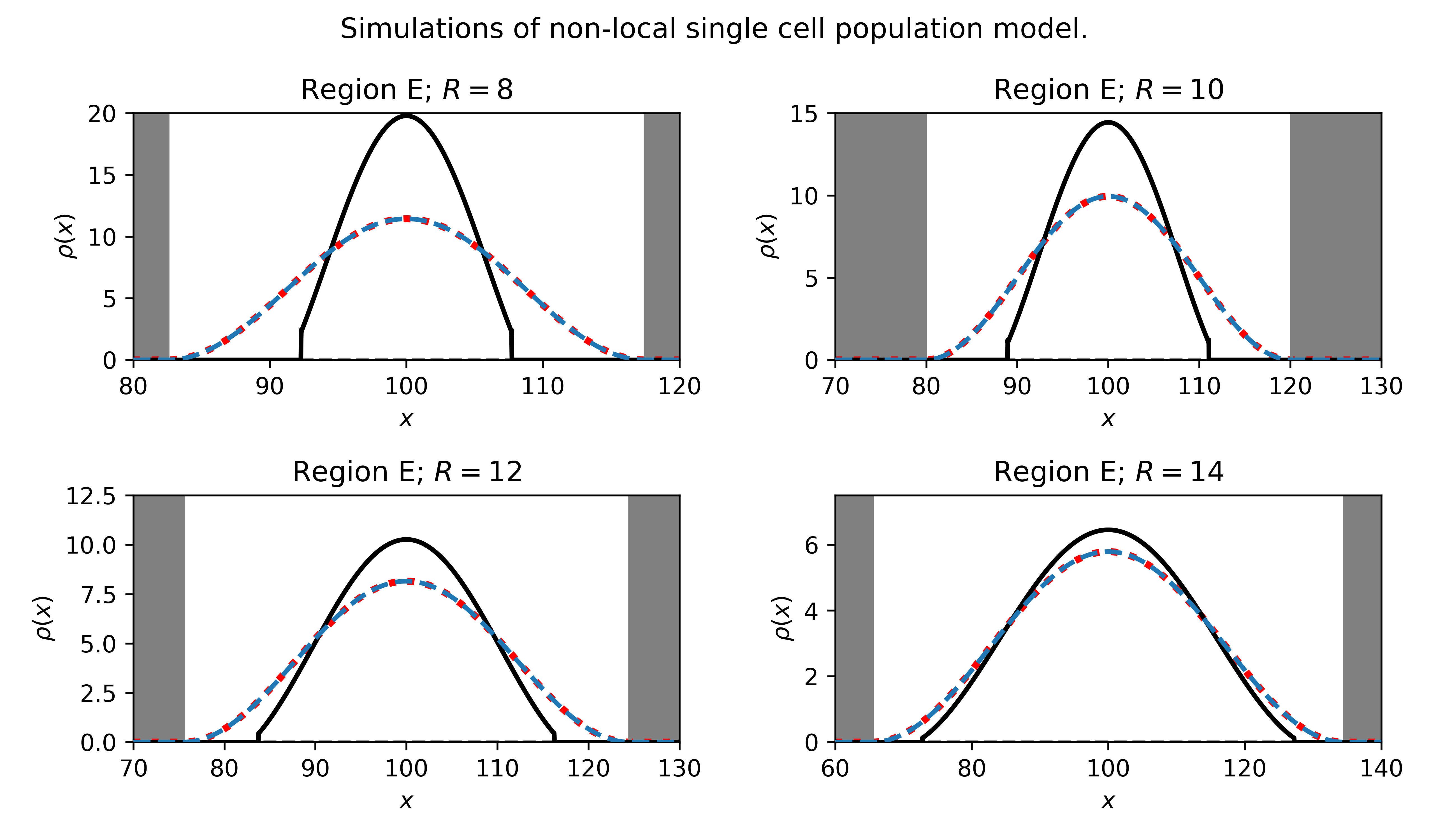
Results are shown in Fig. 7. We plot the numerically simulated cell density profile of the nonlocal model (black), and compare it to the numerically simulated local model (dashed blue) and the analytically predicted steady-state solution (dotted red). The predicted cluster radius is indicated by the width of the white region. We find that the numerical and analytical solutions of the local PDE match one another closely, as seen by the overlapping blue and red curves. However, we find that the local PDE approximation is accurate only in some parameter regimes. In the top two panels, we see that the nonlocal model predicts sharp cluster edges and significant compression compared with the local PDE predictions. Hence the analysis of the local approximation does not exactly match the behaviour of the full nonlocal model. The predicted shape becomes a better approximation as is increased.
8 Discussion
In this paper, we have addressed several questions. First, we examined one example of cellular signaling via diffusible chemotactic chemicals that leads to effective nonlocal cell-cell interactions. This example was first proposed by [28], but has not yet been recognized in recent nonlocal modeling efforts. We showed that when cells secrete a diffusible chemical that decays, and that attracts or repels the cells via the process of chemotaxis, it essentially sets up a “chemical potential” of the Morse type.
Morse potentials have been used in more general settings of cell-cell mechanical interactions in computational biology papers. Morse potentials appear in the context of cell adhesion models [1], as briefly surveyed in Appendix C. [25] used a Morse potential to model adhesive/repulsive interactions of red blood cells (RBCs) in an advanced computational model of RBC aggregation using an immersed finite element method. [39] used a modified Morse potential to represent adhesion of platelets to one another in an ABM model for blood clotting. The Morse potential was adapted to experimental data on shear conditions. [21] used cell tracking in mouse embryos and C. elegans to infer effective mechanical forces and pairwise potential of cell-cell interactions. They showed that Morse potentials were generally a good fit, since tuning the Morse parameters allowed for a range of interactions. They also showed that species differences that implied distinct potential profiles also accounted for tight vs loose cell aggregate morphologies. As discussed in [31], many forms of potentials are reasonable, provided they account for four parameters for magnitudes and spatial ranges of attraction and repulsion, akin to our . Hence, even without the direct link to mechanism, Morse potentials have proven to be convenient approximations for a variety of non-local interactions.
A second question that we addressed is what kinds of attributes chemotactic signals should have to create a robust cell cluster. We showed that the behaviour of cells with attractant and repelent interactions can be classified in a parameter plane where these dimensionless parameters are ratios of magnitudes and spatial ranges of the attractant and repellent. Similar curves were found in [28] in connection with pattern formation criteria. We extended that theory to predict the size of the stable cluster in terms of the chemical properties. We also found the variety of possible behaviours for regions other than that of the cluster formation. In most such regions, the cells cannot aggregate due to dominance of repulsion or the cells collapse due to dominance of attraction.
Some of the theory and predictions here and in [14] rely on the ability to approximate a nonlocal problem by a local PDE, where steady state solutions can be written explicitly and conveniently (at least in 1D). We quantified the degree of accuracy of such local approximations by numerically simulating and comparing the predictions of the nonlocal problem and its local PDE approximation.
Another question of interest is how the continuum results compare with agent based models. Analytic results for the case of a well-spaced swarm (where all agents are at equal distances from neighbors) in [26] arrived at similar regime boundaries in the plane, but did not explore the regime of a loose cluster of finite radius. In [12], the authors investigated an agent-based model for velocity-limited particles that interact with Morse attraction-repulsion kernels. They classified behaviours into “H-stable” (well-spaced group) and “catastrophic” (collapse into a tight cluster), on a parameter plane very similar to the plane shown here. The authors of [24] consider asymptotic dynamics of a 1D swarming model with attraction-repulsion kernels, including the Morse kernel. They show how properties of the kernel’s moments account for whether the group will contract or spread, or form a steady-state cluster. In [36], the authors include self-propulsion, friction, together with attractive/repulsive Morse potential. They assume that the total mass stays constant, regardless of the size of the flock. They numerically simulate their model in 3D, and find regimes for clumps spheres, dispersion, mills, rigid-body rotation, flocks. The above examples have features that go beyond our continuum models, and yet some of the properties that we find persist in these distinct situations.
In future plans for the analysis of collective behaviour, and particularly for the migration of the presypathetic ganglion (PSG) of [20], it would be important to consider the interactions of a second cell type (as modeled in [14]) with similar signaling mechanism, as well as the migration of a cluster towards its target. In such extensions, some analysis is available, though results are not as easily stated, as many new parameters enter the models.
Appendix A Numerical methods
In this section, we give an overview of the numerical methods we employ to solve both the non-local model and its local approximation. In both cases, we solve the partial differential equation
| (35) |
We solve this equation on a large periodic domain . We discretize the equation using a finite volume approach. (See [18] for the theoretical basis.) The non-negative initial condition is
where is a uniformly distributed random variable between . Note that since equation (35) is hyperbolic (i.e. does not contain a smoothing diffusion term) the initial condition must be smooth.
In detail, the spatial term is discretized using a third order upwind scheme with a van Leer flux limiter. It remains to compute the velocities. We consider two cases for the velocities.
-
(a)
In the non-local case we have
The non-local kernel is discretized using the approach outlined in [19]. Most crucially this allows us to use the FFT to evaluate the convolution.
-
(b)
In the local case we have
The first term is discretized as usual, the challenging term here is the second order derivative term. We discretize this term using a second order centered finite difference scheme. This discretization will effectively lead to a second order discretization of a fourth order derivative. For our numerical calculations it is important not to choose the spatial discretization size too small due to the high amplification of round-off errors of this fourth order derivative approximation. We estimate the optimal spatial discretization size as follows
where the first term is the local truncation error and the second term is the rounding error. Minimizing this expression we obtain an optimal discretization size of . Most importantly, discretization sizes below this optimal value lead to the emergence of large round-off errors and are to be avoided.
Appendix B Moments of polynomial repulsion
The moments of the above potential are needed for the local PDE approximation, namely
Simplifying leads to where . Similarly the second moment is
Simplifying results in with . Thus, the moments of the repulsion are similar to those of the Morse repulsive potential, but with some new constants appearing.
Appendix C Morse kernels in adhesion models
Exponential kernels appear in other classes of theoretical models, including non-local adhesion models. For instance, the model proposed by [1] for cell density is
| (36) |
where is the cell’s sensing radius i.e. roughly the distance around the cell over which cell-cell forces are exerted. See also [33, 34, 6]. One common choice of the integral kernel is the exponential
where is a normalization constant. Following the steps in [5], we can write (36) in potential form i.e.
| (37) |
where
In other words, non-local adhesion models (or dispersal models) using Laplace kernels are a type of Morse potential.
References
- \bibcommenthead
- Armstrong et al. [2006] Armstrong, N.J., Painter, K.J., Sherratt, J.A.: A continuum approach to modelling cell–cell adhesion. Journal of theoretical biology 243(1), 98–113 (2006)
- Bessemoulin-Chatard and Filbet [2012] Bessemoulin-Chatard, M., Filbet, F.: A finite volume scheme for nonlinear degenerate parabolic equations. SIAM Journal on Scientific Computing 34(5), 559–583 (2012)
- Byrne and Drasdo [2009] Byrne, H., Drasdo, D.: Individual-based and continuum models of growing cell populations: a comparison. Journal of mathematical biology 58, 657–687 (2009)
- Buttenschön and Edelstein-Keshet [2020] Buttenschön, A., Edelstein-Keshet, L.: Bridging from single to collective cell migration: A review of models and links to experiments. PLoS computational biology 16(12), 1008411 (2020)
- Buttenschön and Hillen [2021] Buttenschön, A., Hillen, T.: Non-local cell adhesion models: Steady states and bifurcations (2021)
- Buttenschön et al. [2018] Buttenschön, A., Hillen, T., Gerisch, A., Painter, K.J.: A space-jump derivation for non-local models of cell–cell adhesion and non-local chemotaxis. Journal of mathematical biology 76, 429–456 (2018)
- Bonner [1998] Bonner, J.T.: A way of following individual cells in the migrating slugs of dictyostelium discoideum. Proceedings of the National Academy of Sciences 95(16), 9355–9359 (1998)
- Bernoff and Topaz [2016] Bernoff, A.J., Topaz, C.M.: Biological aggregation driven by social and environmental factors: A nonlocal model and its degenerate cahn–hilliard approximation. SIAM Journal on Applied Dynamical Systems 15(3), 1528–1562 (2016)
- Chitnis et al. [2012] Chitnis, A.B., Dalle Nogare, D., Matsuda, M.: Building the posterior lateral line system in zebrafish. Developmental neurobiology 72(3), 234–255 (2012)
- Costa Filho et al. [2013] Costa Filho, R.N., Alencar, G., Skagerstam, B.-S., Andrade, J.S.: Morse potential derived from first principles. Europhysics Letters 101(1), 10009 (2013)
- Chaplain et al. [2020] Chaplain, M.A., Lorenzi, T., Macfarlane, F.R.: Bridging the gap between individual-based and continuum models of growing cell populations. Journal of Mathematical Biology 80(1), 343–371 (2020)
- D’Orsogna et al. [2006] D’Orsogna, M.R., Chuang, Y.-L., Bertozzi, A.L., Chayes, L.S.: Self-propelled particles with soft-core interactions: patterns, stability, and collapse. Physical review letters 96(10), 104302 (2006)
- Elliott and Garcke [1996] Elliott, C.M., Garcke, H.: On the cahn–hilliard equation with degenerate mobility. SIAM journal on mathematical analysis 27(2), 404–423 (1996)
- Falcó et al. [2023] Falcó, C., Baker, R.E., Carrillo, J.A.: A local continuum model of cell-cell adhesion. SIAM Journal on Applied Mathematics, 17–42 (2023)
- Friedl and Mayor [2017] Friedl, P., Mayor, R.: Tuning collective cell migration by cell–cell junction regulation. Cold Spring Harbor perspectives in biology 9(4), 029199 (2017)
- Friedl et al. [1995] Friedl, P., Noble, P.B., Walton, P.A., Laird, D.W., Chauvin, P.J., Tabah, R.J., Black, M., Zänker, K.S.: Migration of coordinated cell clusters in mesenchymal and epithelial cancer explants in vitro. Cancer research 55(20), 4557–4560 (1995)
- Gerisch and Chaplain [2008] Gerisch, A., Chaplain, M.A.: Mathematical modelling of cancer cell invasion of tissue: local and non-local models and the effect of adhesion. Journal of theoretical biology 250(4), 684–704 (2008)
- Gerisch [2001] Gerisch, A.: Numerical methods for the simulation of taxis diffusion reaction systems. PhD thesis, Martin-Luther-Universitat Halle-Wittenberg (2001)
- Gerisch [2010] Gerisch, A.: On the approximation and efficient evaluation of integral terms in pde models of cell adhesion. IMA Journal of Numerical Analysis 30(1), 173–194 (2010)
- Kasemeier-Kulesa et al. [2015] Kasemeier-Kulesa, J.C., Morrison, J.A., Lefcort, F., Kulesa, P.M.: Trkb/bdnf signalling patterns the sympathetic nervous system. Nature communications 6, 8281 (2015)
- Koyama et al. [2023] Koyama, H., Okumura, H., Ito, A.M., Nakamura, K., Otani, T., Kato, K., Fujimori, T.: Effective mechanical potential of cell–cell interaction explains three-dimensional morphologies during early embryogenesis. PLoS Computational Biology 19(8), 1011306 (2023)
- Keller and Segel [1971] Keller, E.F., Segel, L.A.: Model for chemotaxis. Journal of theoretical biology 30(2), 225–234 (1971)
- Knutsdottir et al. [2017] Knutsdottir, H., Zmurchok, C., Bhaskar, D., Palsson, E., Dalle Nogare, D., Chitnis, A.B., Edelstein-Keshet, L.: Polarization and migration in the zebrafish posterior lateral line system. PLoS computational biology 13(4), 1005451 (2017)
- Leverentz et al. [2009] Leverentz, A.J., Topaz, C.M., Bernoff, A.J.: Asymptotic dynamics of attractive-repulsive swarms. SIAM Journal on Applied Dynamical Systems 8(3), 880–908 (2009)
- Liu et al. [2004] Liu, Y., Zhang, L., Wang, X., Liu, W.K.: Coupling of navier–stokes equations with protein molecular dynamics and its application to hemodynamics. International Journal for Numerical Methods in Fluids 46(12), 1237–1252 (2004)
- Mogilner et al. [2003] Mogilner, A., Edelstein-Keshet, L., Bent, L., Spiros, A.: Mutual interactions, potentials, and individual distance in a social aggregation. Journal of mathematical biology 47, 353–389 (2003)
- Merchant et al. [2018] Merchant, B., Edelstein-Keshet, L., Feng, J.J.: A rho-gtpase based model explains spontaneous collective migration of neural crest cell clusters. Developmental biology 444, 262–273 (2018)
- Mogilner [1995] Mogilner, A.: Modelling spatio-angular patterns in cell biology. PhD thesis, University of British Columbia (1995)
- Marée et al. [1999] Marée, A.F., Panfilov, A.V., Hogeweg, P.: Migration and thermotaxis of dictyostelium discoideum slugs, a model study. Journal of theoretical biology 199(3), 297–309 (1999)
- Murray [2003] Murray, J.D.: Mathematical Biology: II: Spatial Models and Biomedical Applications vol. 18. Springer, New York (2003)
- Newman [2005] Newman, T.J.: Modeling multi-cellular systems using sub-cellular elements. arXiv preprint q-bio/0504028 (2005)
- Othmer and Hillen [2002] Othmer, H.G., Hillen, T.: The diffusion limit of transport equations ii: Chemotaxis equations. SIAM Journal on Applied Mathematics 62(4), 1222–1250 (2002)
- Painter et al. [2010] Painter, K.J., Armstrong, N.J., Sherratt, J.A.: The impact of adhesion on cellular invasion processes in cancer and development. Journal of theoretical biology 264(3), 1057–1067 (2010)
- Painter et al. [2015] Painter, K.J., Bloomfield, J., Sherratt, J., Gerisch, A.: A nonlocal model for contact attraction and repulsion in heterogeneous cell populations. Bulletin of mathematical biology 77, 1132–1165 (2015)
- Palsson and Othmer [2000] Palsson, E., Othmer, H.G.: A model for individual and collective cell movement in dictyostelium discoideum. Proceedings of the National Academy of Sciences 97(19), 10448–10453 (2000)
- Vecil et al. [2013] Vecil, F., Lafitte, P., Linares, J.R.: A numerical study of attraction/repulsion collective behavior models: 3d particle analyses and 1d kinetic simulations. Physica D: Nonlinear Phenomena 260, 127–144 (2013)
- Weijer [2009] Weijer, C.J.: Collective cell migration in development. Journal of cell science 122(18), 3215–3223 (2009)
- Weiner et al. [1997] Weiner, R., Schmitt, B.A., Podhaisky, H.: Rowmap–a row-code with krylov techniques for large stiff odes. Applied Numerical Mathematics 25, 303–319 (1997)
- Yazdani et al. [2017] Yazdani, A., Li, H., Humphrey, J.D., Karniadakis, G.E.: A general shear-dependent model for thrombus formation. PLoS computational biology 13(1), 1005291 (2017)