Hot subdwarf Atmospheric parameters, Kinematics, and Origins – Based on 1587 hot subdwarf stars observed in Gaia DR2 and LAMOST DR7
Abstract
Based on the Gaia DR2 catalogue of hot subdwarf star candidates, we identified 1587 hot subdwarf stars with spectra in LAMOST DR7. We present atmospheric parameters for these stars by fitting the LAMOST spectra with Tlusty/Synspec non-LTE synthetic spectra. Combining LAMOST radial velocities and Gaia Early Data Release 3 (EDR3) parallaxes and proper motions, we also present the Galactic space positions, velocity vectors, orbital parameters and the Galactic population memberships of the stars. With our He classification scheme, we identify four groups of He rich hot subdwarf stars in the and diagrams. We find two extreme He-rich groups (He-1 and He-2) for stars with and two intermediate He-rich groups (He-1 and He-2) for stars with . We also find that over half of the stars in Group He-1 are thick disk stars, while over half of the stars in Group He-2 correspond to thin disk stars. The disk population fractions of Group He-1 are between those of Group He-1 and He-2. Almost all stars in Group He-2 belong to the thin disk. These differences indicate that the four groups probably have very different origins. Comparisons between hot subdwarf stars in the halo and in the Galactic globular cluster Cen show that only He-deficient stars with have similar fractions. Hot subdwarfs with in Cen have no counterparts in the thick disk and halo populations, but they appear in the thin disk.
1 Introduction
Hot subdwarf stars are evolved core He burning stars with thin H envelopes on the extreme horizontal branch (EHB, Heber 2009, 2016). Their spectral features are similar to that of typical O/B type stars, but their luminosities are orders of magnitudes lower. They are classified according to their spectral features into sdB and sdO types (Drilling et al., 2013). Hot subdwarf stars are interesting objects in many fields of astronomy. They are found in all galactic populations, and they are known to be the main source of the ultraviolet excess radiation of elliptical galaxies and the bulges of spiral galaxies (Han et al., 2007), and also responsible for the extended horizontal branch morphology of globular clusters (Han, 2008; Lei et al., 2013, 2015). Hypervelocity hot subdwarf stars allow us to probe the Galactic gravitational potential and put constraints on the mass of the Galactic dark matter halo (Geier et al., 2015; Németh et al., 2016). The orbital-period - mass-ratio (P-q) relation in wide hot subdwarf binaries reflects the Galactic history (Vos et al., 2020). Hot subdwarf binaries with massive compact companions play a role as progenitors of cosmologically important type Ia supernovae (Justham et al., 2009; Wang et al., 2009; Wang & Han, 2010; Geier et al., 2013, 2015; Ratzloff et al., 2020) and mark potential gravitational-wave sources, that may be strong enough to be detectable by future space-based missions, such as the Laser Interferometer Space Antenna (Wu et al., 2018, 2020).
Hot subdwarf stars are excellent probes for binary evolution, stellar atmosphere and interior models. Because a large fraction of sdB stars must have gone through a common-envelope (CE) phase of evolution and are detached binaries, they provide a clean-cut laboratory to study this poorly understood, yet crucial phase of binary evolution and tidal effects (Ivanova et al., 2013; Pelisoli et al., 2020; Han et al., 2020). Hot subdwarf stars display strong chemical peculiarities, in particular for the He abundance, which may be a trace element as well as the dominant constituent of the atmosphere, depending on the hot subdwarf type (Edelmann et al., 2003; Németh et al., 2012; Byrne et al., 2018). Furthermore, the atmospheres of a few intermediate He-rich hot subdwarfs show extreme heavy metal abundances, with abundances of lead reaching nearly 10 000 times the solar value, that is 10-100 times higher than that previously measured in normal hot subdwarf atmospheres (Naslim et al., 2011, 2013, 2020; Jeffery et al., 2017; Jeffery & Miszalski, 2019; Latour et al., 2018; Saio & Jeffery, 2019; Dorsch et al., 2019, 2020; Fernández-Menchero et al., 2020). Several types of pulsating stars have been discovered among hot subdwarfs, being remarkable targets for asteroseismology to probe their interior structure (Charpinet et al., 2010; Zong et al., 2018; Kupfer et al., 2019; Sahoo et al., 2020; Jeffery, 2020; Østensen et al., 2014, 2020).
Despite their importance in many fields of astronomy, the formation of hot subdwarfs is, in general, still unclear. They can be formed only if the progenitor loses its envelope almost entirely after passing the red giant branch. Different scenarios have been proposed to explain the huge mass loss. There are three main such scenarios for hot subdwarf stars: The common envelope (CE) ejection (Webbink, 1984), the stable Roche lobe overflow (RLOF) and the merger of double helium white dwarfs (HeWD) (Han et al., 2002). Population synthesis studies show that the first two channels produce hot subdwarfs in binary systems and the last one creates single He-rich sdO stars (Han et al., 2003; Han, 2008; Zhang & Jeffery, 2012). In the transition between the sdB and sdO types both the late hot-flasher scenario (D’Cruz et al., 1996; Moehler et al., 2004; Miller Bertolami et al., 2008) and the merger of helium white dwarfs with low mass main sequence stars (Zhang et al., 2017) have been identified as a viable formation channel for some intermediate He-rich (He) hot subdwarf stars.
Up to now, there is not a single formation theory that could simultaneously explain all the observed features and distributions of hot subdwarf stars. With the advent of the Gaia survey (Gaia Collaboration et al., 2016) and new spectroscopic surveys like LAMOST (Cui et al., 2012) (the Large Sky Area Multi-Object Fiber Spectroscopic Telescope, also named the ”Guo Shou Jing” Telescope), we can characterize the details of hot subdwarfs by combining kinematic and spectroscopic properties of large observed samples. By combing Gaia DR2 and LAMOST DR5, we presented the spectral analyses of 892 non-composite spectra hot subdwarf stars and the kinematics of 747 stars and revealed that hot subdwarfs can be further divided into four He groups that correlate with different formation channels (Luo et al., 2019). Most recently, Luo et al. (2020) studied the kinematics of 182 single-lined hot subdwarfs selected from Gaia DR2 with spectra from LAMOST DR6 and DR7 (Lei et al., 2020) and confirmed our results reported by Luo et al. (2019). Although 39 800 hot subdwarf candidates were selected by Geier et al. (2019), the properties of the majority of the stars are still unknown.
In this paper, a total of 1587 hot subdwarf stars are identified from the Gaia DR2 hot subdwarf candidate catalog (Geier et al., 2019) with LAMOST DR7 spectra, among which, there are 224 new hot subdwarfs, which are confirmed here the first time. We performed a spectral and kinematical analysis of all 1587 hot subdwarfs with LAMOST DR7 spectra using their Gaia EDR3 parallaxes and proper motions. The catalogue of 1587 hot subdwarf stars includes RVs, atmospheric parameters, as well as Galactic space positions, space motions, orbital parameters and Galactic population classifications. The paper is organized as follows: Our data and sample selection are described in Sect 2. The methods to derive atmospheric parameters, Galactic space velocities and orbital parameters are explained in Sect 3 and 4. This is followed by our results on the properties of atmospheric parameters, Galactic space distributions, Galactic velocity distributions, Galactic orbits and Galactic population classifications in Sect 5. Then we make a discussion in Sect 6, before summarizing and concluding our work in Sect 7.
2 Data and sample selection
2.1 Data
LAMOST is a 4-m specially designed Schmidt spectroscopic survey telescope, which can simultaneously observe 4000 targets per exposure in a field of view of about in diameter (Cui et al., 2012; Luo et al., 2012). LAMOST spectra are similar to SDSS data and cover the wavelength range of Å with a resolution of . In March 2020, LAMOST has released 10 608 416 spectra in DR7, which is described and available at: http://dr7.lamost.org/
Gaia is a European Space Agency space telescope that maps the positions and motions of more than 1 billion stars to the highest precision yet of any missions (Gaia Collaboration et al., 2016). On April 25, 2018, Gaia DR2 was released, which provides high-precision positions ( and ), proper motions ( and ) and parallaxes () as well as three broadband magnitudes (, and ) for over 1.3 billion stars brighter than mag (Gaia Collaboration et al., 2018). For the vast majority of stars in Gaia DR2, a reliable distance cannot be obtained by simply inverting the parallax, . Bailer-Jones et al. (2018) presented a Gaia DR2 distance catalogue by estimating distances from parallaxes. Gaia EDR3 (Gaia Collaboration et al., 2020) was released on December 3, 2020 and significantly improved the precision and accuracy of astrometry and broad-band photometry over Gaia DR2. Gaia EDR3 contains astrometry and photometry for 1.8 billion sources brighter than mag. For 1.5 billion of those sources, parallaxes (), proper motions ( and ) and the colours are available. Bailer-Jones et al. (2021) also provided a Gaia-EDR3 distance catalogue based on Gaia EDR3. Therefore, where necessary, unreliable distances were replaced with the estimated values from the Gaia-DR3 distance catalogue (Bailer-Jones et al., 2021).
2.2 Sample selection
Based on Gaia DR2 data, Geier et al. (2019) compiled an all-sky catalogue of 39 800 hot subdwarf candidates by using the means of colour, absolute magnitude and reduced proper motion cuts. Luo et al. (2020) showed that most of those objects lie between 500 pc and 1500 pc distance and the catalogue is nearly volume complete. By cross-matching the catalogue with LAMOST DR7, we selected 2595 stars from the Gaia DR2 catalogue of hot subdwarf candidates. After rejecting bad spectra, MS stars, WDs, and objects with strong Ca ii H&K ( Å and Å), Mg i ( Å), or Ca ii ( Å) absorption lines, we obtained 1587 stars with a spectral signal-to-noise (S/N) over 10 in the -band, by visually comparing them with reference spectra of hot subdwarf stars. 224 stars are confirmed as hot subdwarfs for the first time. Figure 1 shows the positions of these 1587 stars in the Gaia HR diagram and Table 1 lists the proper motions and distances derived from Gaia EDR3 parallaxes. However, for 74 stars reliable distances could not be calculated by inverting a negative parallax. Therefore, we replaced their distances with the estimated values from the Gaia-EDR3 distance catalogue (Bailer-Jones et al., 2021). Additionally, Table 2 lists 665 targets removed from the Gaia DR2 catalogue of hot subdwarf candidates with LAMOST spectra with in the -band. Most of these candidates were misclassified as hot subdwarfs.
Figure 2 illustrates distribution functions of the absolute Gaia magnitudes of hot subdwarf stars with a distance between 500 pc and 1500 pc in Gaia DR2 and LAMOST DR7. The similar distributions suggest that the sample of hot subdwarfs in LAMOST DR7 is a representative and unbiased sub-sample of the volume-complete Gaia sample. We consider all stars to be members of the thin disk, thick disk or halo populations until they can be further constrained. Unknown and unresolved binary systems affect the calculations of Galactic velocities and orbits. Although our study focuses on studying only single-lined hot subdwarf stars, based on a single epoch radial velocity measurement we cannot exclude the possibility of having unknown and unresolved binary systems in our sample. Our simulations (Luo et al., 2020) have demonstrated that the impact of an RV variability as a selection effect on the population classification propagates to less than 5% relative differences in the number of stars in a He-group.
3 Atmospheric parameters
3.1 Model atmospheres
All model atmospheres were computed with the non-LTE (non-local thermodynamic equilibrium) code Tlusty (Hubeny & Lanz, 1995), version 205. The corresponding hot subdwarf synthetic spectra were created using the spectrum synthesis code Synspec (Hubeny & Lanz, 2011), version 51. Further details of these codes are available in the newest user’s manuals (Hubeny & Lanz, 2017a, b, c). Model atmospheres were calculated under the standard assumptions of plane-parallel, horizontally homogeneous atmospheres in hydrostatic and radiative equilibrium. Pure H+He chemical compositions were assumed for all models. The broadening of H line profiles were calculated using the tables of Tremblay & Bergeron (2009) that take into account the effects of level dissolution directly in the evaluation of line profiles. Four detailed He i line profiles (, , and Å) were taken from the special line broadening tables of Mihalas et al. (1974) and He ii line profiles were taken from the Stark broadening tables of Schoening & Butler (1989).
3.2 Spectral analysis
The radial velocities provided in the LAMOST catalog are not reliable for hot subdwarf stars, because hot subdwarfs are not included in the LAMOST stellar template library. Therefore, we measured new radial velocities using our synthetic spectra as templates and list these velocities in Table 1. Following the works of Luo et al. (2016, 2019), atmospheric parameters (effective temperature , surface gravity , and He abundances ) were obtained by fitting the observed data with a grid of synthetic spectra. The synthetic spectra were degraded to the resolution of LAMOST data and normalized in 80 Å sections to the LAMOST flux-calibrated observations. We used the wavelength range of Å, which includes all significant H and He lines in the LAMOST spectra. We employed the library for non-linear least-squares minimization and curve-fitting for Python (LMFIT) to determine the best-fit values of the parameters and estimate the standard errors. We used the Levenberg-Marquardt minimization method of the LMFIT package in our fitting procedure.
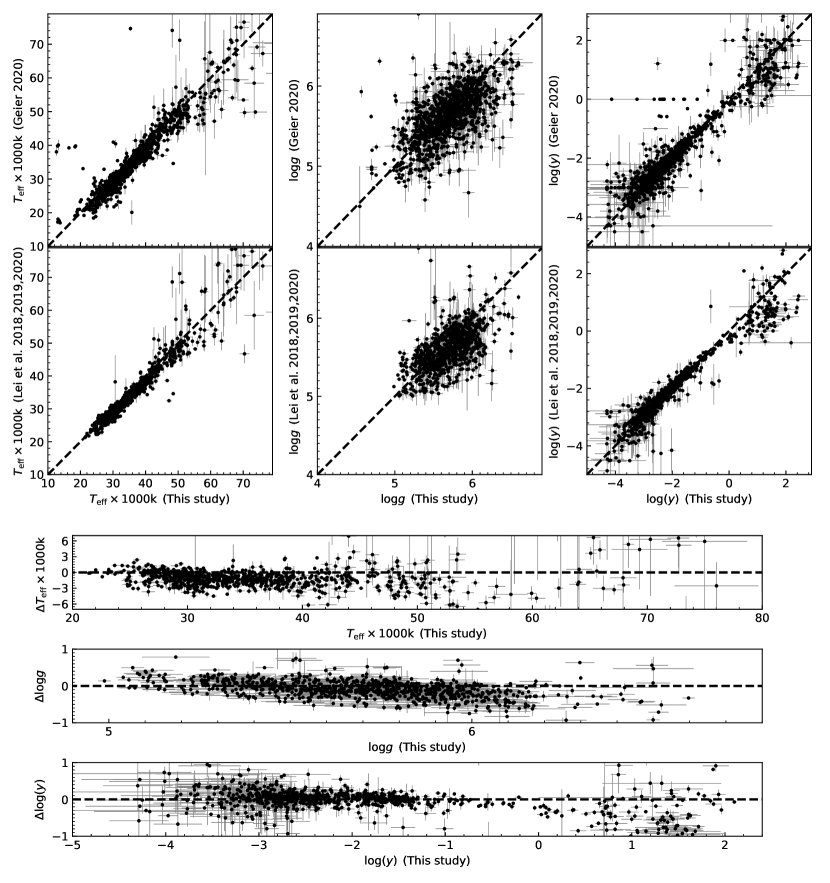
Table 1 lists the atmospheric parameters derived from the spectra of the 1587 hot subdwarf stars. We cross-matched our results with the latest catalogue of known hot subdwarf stars (Geier, 2020) and obtained 1363 stars in common. , , and are simultaneously available for 1195 common stars. The top three panels of Figure 3 show comparisons of the atmospheric parameters of these stars between our study and Geier (2020). The derived and are similar in both of these studies. The largest deviations appear above 55 000 K, where both non-LTE effects and model composition play an important role. For the He abundance the largest errors are random errors at the lowest and highest He abundances. Surface gravity is different, though. Instead of a linear correlation, it shows an elongated blob. The surface gravity is particularly difficult to measure with precision from H+He models and low resolution observations, and this affects both studies in our comparison. Although the values show a larger dispersion than the former two parameters, our results agree with the values from Geier (2020) and the error bars are also comparable. We note that our error bars are 1 errors (68% confidence), while the collection of Geier (2020) also includes samples calculated for 60% confidence. There are 852 stars in the sample of Lei et al. (2018, 2019, 2020), which were analysed by applying the same model atmospheres (Tlusty) on the same spectra, but a different fitting procedure. The bottom three panels of Figure 3 show the atmospheric parameter comparisons between our study with Lei et al. (2018, 2019, 2020). is quite similar for these stars. agrees with results of Lei et al. (2018, 2019, 2020) for stars with while it shows a linear offset for stars with . As shown in above results, shows exhibits a larger dispersion than the former two parameters. It is reassuring that the largest systematic differences are observed at hot, He dominated stars, which require more complex models.
4 Calculations of Galactic space velocities and orbital parameters
Combining the parallaxes and proper motions published by Gaia EDR3 and the RV measured from the spectra of LAMOST DR7, we calculated the space velocity components of hot subdwarf stars in the right-handed Galactocentric Cartesian coordinate system with the Astropy Python package. We took the usual convention of the space velocity components , , and oriented towards the Galactic center, the direction of Galactic rotation and the north Galactic pole, respectively. We adopted the distance of the Sun from the Galactic center to be 8.4 kpc and the velocity of the local standard of rest (LSR) to be (Irrgang et al., 2013). For the solar velocity components with respect to the LSR, we took (, , )(11.1, 12.24, 7.25) (Schönrich et al., 2010). Using Astropy, we also computed the space position components (, , ) in a right-handed Galactocentric Cartesian reference frame.
The Galactic orbits were computed using the Galpy Python package (Bovy, 2015). We integrated orbits in Galpy ”MWpotential2014” potential that comprises a power-law bulge with an exponential cut-off, an exponential disk and a power-law halo component (Bovy, 2015), using the same Galactocentric distance of the Sun and the same LSR as in Astropy. The time of orbital integration was set from 0 to Gyr in steps of Myr. The Galactic orbital parameters of hot subdwarf stars, such as the apocentre (), pericentre (), eccentricity (), maximum vertical amplitude (), normalised z-extent () and z-component of the angular momentum (), were extracted from integrating their orbital paths. and denote the maximum and minimum distances of an orbit from the Galactic center, respectively. We defined the eccentricity by
| (1) |
and the normalised z-extent by
| (2) |
where is the Galactocentric distance.
The space positions and velocity components, as well as the orbital parameters are listed in Table 1. The errors of these parameters were estimated with a Monte Carlo (MC) method. For each star, 1000 random input values with a Gaussian distribution were simultaneously performed and the output parameters were computed together with their errors. Further details on the parameter error calculations were presented by Luo et al. (2019).
5 Results
5.1 The atmospheric properties of the stars
Figure 5 exhibits the distribution of hot subdwarf stars in the diagram. The zero-age HB (ZAHB) and terminal-age HB (TAHB) calculated by Dorman et al. (1993) and the zero-age He main sequence given by Paczyński (1971) are marked in the figure. Three sdB evolutionary tracks of Dorman et al. (1993) for solar metallicity and a subdwarf core mass of are plotted in Figure 5.
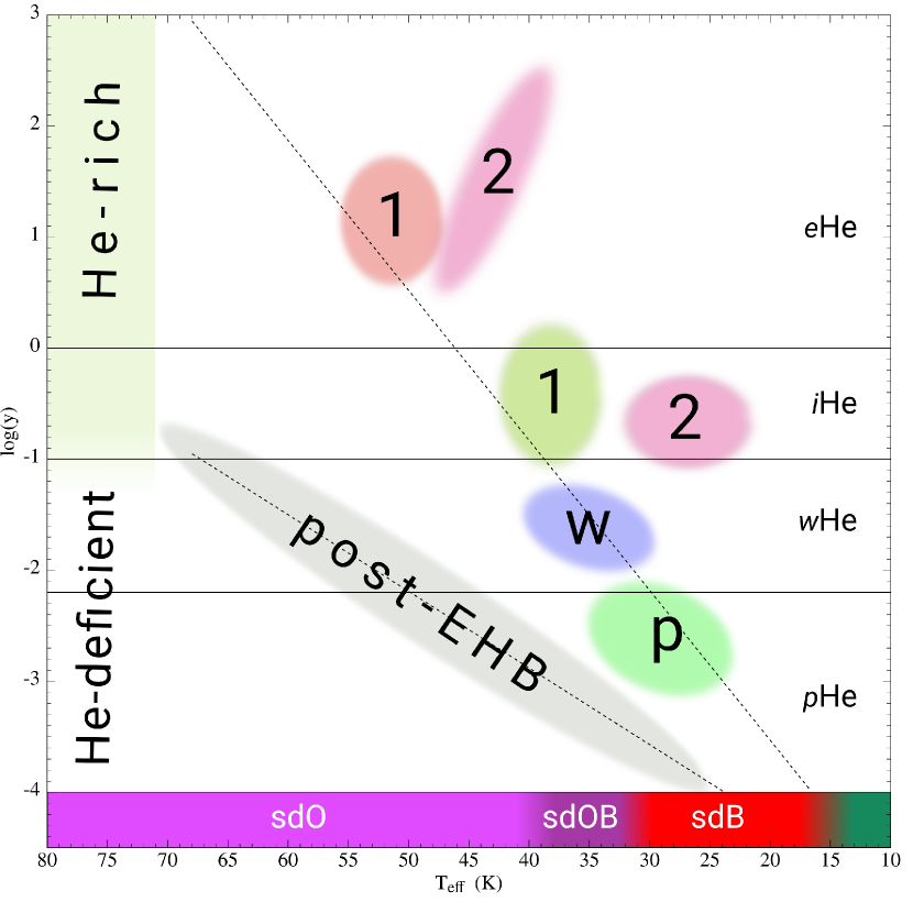
Following our helium abundance classification scheme, hot subdwarf stars are divided into He-rich and He-deficient stars with respect to the solar He abundance . Both He-rich and He-deficient stars are then further divided into two classes (He abundance classes) via and , respectively. As described by Németh et al. (2012) and Luo et al. (2019), our classification scheme associates these classes with distinct formation channels in the diagram. In this paper, He-rich stars with are marked as the extreme He-rich (He) stars while He-rich stars with are named as intermediate He-rich (He) stars. We refer to He-deficient stars with as He-weak (He) and stars as He-poor (He) stars. Within the four He abundance classes, we distinguish groups of stars that show characteristically different atmospheric and kinematic properties. Figure 4 gives a schematic overview of the He abundance classification system.
In Figure 5, four classes of hot subdwarf stars can be outlined by using our He abundance classification scheme. As reported in previous studies (Németh et al., 2012; Luo et al., 2016, 2019), two He-deficient sdB groups are located on the EHB and they correspond to potential mode and mode pulsating sdB stars. However, the correspondence between pulsation and atmospheric properties are not yet clear and only a tiny fraction of He-deficient stars are pulsators, therefore we distinguish these groups by the He abundance. One group consists of He-poor (He) stars with near K and cm s-2. Another group consists of He-weak (He) stars with near K and cm s-2. The former group is on average 10 times less He abundant than the latter. He-rich stars () also show two classes at higher He abundances. One class is composed of He-sdO/sdB stars () between K and K and another class consists of the He-rich sdO/sdB stars () near K and cm s-2. These results are in agreement with the observations of Németh et al. (2012) and Luo et al. (2016, 2019).
The left panel of Figure 6 illustrates the distribution of He-rich hot subdwarf stars in the diagram. Two evolutionary tracks with solar metallicity for subdwarf masses of and from the double WD merger channels of Zhang & Jeffery (2012) are also marked. It is clearly seen that He-rich stars with show a gap near K in the diagram, which were reported in several studies (Stroeer et al., 2007; Hirsch, 2009; Kepler et al., 2019). Two groups (He-1 and He-2) of He-rich stars with can be outlined by the gap. They cluster either near K and cm s-2, or near K and cm s-2, respectively. When compared to evolutionary tracks of hot subdwarf stars through the double WD merger model (Zhang & Jeffery, 2012), the evolutionary tracks match these two groups. Therefore, Group He-1 we associated with the fast merger channel and Group He-2 with the slow merger channel in the merger model of Zhang & Jeffery (2012).
At higher temperature, the majority of He-rich stars with cluster near K and cm s-2 and define Group He-1. At lower temperature, we find 12 He-rich stars with , near K and cm s-2 in the diagram and outlines the newly discovered Group He-2. Although He-rich stars with and K did not show up as a clear group in LAMOST DR5, one can see that in the current, and larger sample, 5 stars are found in the region of Group He-2. The right panel of Figure 6 compares evolutionary tracks for hot subdwarfs via the hot-flasher scenario (Miller Bertolami et al., 2008) for three stellar surface mixing: Hot-flasher with no He enrichment, hot-flasher with shallow mixing (SM), and hot-flasher with deep mixing (DM). It appears that these evolutionary tracks not only match Group He-1 and He-2 at lower temperatures, but also cover Group He-2 at higher temperature.
Figure 7 displays the distribution of hot subdwarf stars in the diagram. As reported by other authors (Edelmann et al., 2003; Németh et al., 2012; Luo et al., 2019), our sample also shows two distinct He sequences with a clear trend of increasing He abundance with effective temperature. To make a comparison with previous results we plot the two best-fit trends in Figure 7, that are described by the following relationships:
| (3) |
| (4) |
Where the former is taken from Edelmann et al. (2003) and the latter is from Németh et al. (2012). The first best-fit trend is able to match He-deficient stars in the first sequence, but it is not suitable for He-rich stars. As reported by other authors (Hirsch, 2009; Németh et al., 2012), He-rich stars with follow an opposite trend: The He abundance decreases with temperature and approaches , and He-rich stars with deviate progressively from the best-fit trend with increasing temperature. Moreover, the four groups of He-rich stars identified in the diagram can be clearly outlined in the diagram as well. They lie near or above the first sequence (Eqn 3) and are clearly marked by four ellipses in the diagram. Form the diagram, one can see that 11 stars with are near Group He-1, and 5 stars with are near Group He-2. They are outlined as Group He-1 and He-2, respectively. He-rich stars aggregate in four regions in the and diagrams. As shown in Figure 7, the four groups can be defined by the four ellipses and they are well separated by the observed gaps in the diagram. Groups He-1 and He-2 show significantly different trends in He abundance: with the increase of temperature, the He abundance of Group He-2 declines linearly to the value of Group He-1. The He abundance of Group He-1 is nearly independent of temperature. A similar result was reported by Jeffery et al. (2021). The number of stars in Group He-1 and He-2 display a significant difference: the former group has 65 members, but the later includes only 17 stars. The He abundance of Group He-1 is on average somewhat higher than that of Group He-2.
5.2 Space distribution
Figure 8 exhibits the space positions of the four hot subdwarf helium abundance classes and four groups in the diagrams, in which the black dashed lines mark kpc, which corresponds to the vertical scale height of the thick disk (Ma et al., 2017). The upper left panel of Figure 8 displays that two He-deficient groups have nearly the same space position distributions. About of the stars lie within kpc. Based on the upper right panel of Figure 8, the two He-rich groups do not display any clear differences in space position distribution and about the stars lie within kpc. However, we find difference between the relative number of He-rich and He-deficient stars (upper left and right panels) with kpc, which implies that He-rich and He-deficient hot subdwarfs have different kinematic origins.
The lower left panel of Figure 8 shows that of the stars in Group He-1 are found at kpc, but Group He-2 has about of the stars in this region. The lower right panel of Figure 8 reveals that of the stars in Group He-1 are located at kpc, while in Group He-2 all stars are in this region. These observations suggest that all four groups of He-rich stars may have different kinematic origins or formation channels.
5.3 Galactic velocity distribution
Figure 9 displays the distribution of the four hot subdwarf helium classes and four He-rich groups in the velocity diagram. In order to understand their kinematic origins, we also plot the two dashed ellipses as presented in Figure 1 of Martin et al. (2017). They represent the limits of thin and thick disk WDs (Pauli et al., 2006), respectively.
The upper left panel of Figure 9 exhibits that of He-deficient stars are located within the limits of the thin-disk, lie between the limits of thin and thick-disk and the remaining are located outside the limits of thick-disk stars. The upper right panel of Figure 9 displays that the fractions of He-rich stars in the three regions defined above are , and , respectively. Comparisons between the upper panels of Figure 9 demonstrate that the fraction of He-rich stars in the halo population is higher than that of He-deficient stars, which agrees with the results we found from the space distribution of stars in the preceding section. These observations support that He-rich and He-deficient stars have different kinematic origins.
The lower left panel of Figure 9 shows a comparison between Group He-1 and He-2 of He-rich stars with . There are of stars in Group He-1 within the limits of the thin-disk, between the limits of the thin and thick disk, and the remaining are out of the limits of the thick-disk. But Group He-2 shows a quite different distribution, where , and correspond to these three regions, respectively. It can be concluded that stars in Group He-1 and He-2 mainly form in the thick and thin disk, respectively. From the lower right panel of Figure 8, one can see that , , stars in Group He-1 are located above three corresponding regions and almost all stars () of Group He-2 lie within the limits of the thin-disk. Again, these results support that the four He-rich groups have different kinematic origins.
Table 3 lists the mean values and dispersions of the Galactic velocities of the four He classes and four He-rich groups. Intermediate He-rich stars with show the largest velocity dispersion values and He-rich stars with exhibit the second largest velocity dispersion. This result is consistent with the findings of Martin et al. (2017) but in disagreement with our previous results (Luo et al., 2019, 2020). Thanks to the significant improvements in the astrometric precision and accuracy of EDR3, more He-rich stars with are identified now as halo stars. The two groups of He-deficient sdB stars show similar dispersions, and their mean values are less than those of He-rich stars, which further supports that He-deficient and He-rich stars have different kinematic origins. The velocity dispersion of Group He-1 is larger than of Group He-2, but nearly equal to Group He-1. Group He-2 exhibits the smallest velocity dispersion. It can be concluded that the diverse range of kinematic velocities supports the different origins of the four He-rich groups.
5.4 Galactic orbits
Both the z-component of the angular momentum and the eccentricity of the orbit are two important orbital parameters for characterising the kinematics of hot subdwarf stars. Figure 10 shows the distribution of the four hot subdwarf He abundance classes and four groups in the diagram. In Figure 10, we plot the two regions defined by Pauli et al. (2003). Region A encompasses thin disk stars clustering in an area of low eccentricity and around , while Region B encompasses thick disk stars having higher eccentricities and lower angular momenta. Outside of these two regions, defined here as region C, halo star candidates are found.
As reported by Luo et al. (2020), the majority of stars in the upper two panels of Figure 10 show a continuous distribution from Region A to Region B without any obvious dichotomy. Only a few stars are found in Region C and He-rich stars with have a very high fraction in this region. The lower two panels of Figure 10 illustrate that Group He-1 has a higher number fraction in Region C than Group He-2, but the situation is the opposite in Region A. Group He-1 has a lower fraction than both Group He-1 and He-2 in Region B. All stars in Group He-2 have lower eccentricities and higher angular momenta and are found in Region A.
Table 2 displays the mean values and standard deviations of the orbital parameters: eccentricity, z-component of the angular momentum, normalised z-extent, maximum vertical amplitude, apocentre and pericentre. Intermediate He-rich stars with show the largest dispersion of the orbital parameters and He-rich stars with display the second largest velocity dispersion. The two groups of He-deficient sdB stars show similar velocity dispersions. These results are in good agreement with the findings of Martin et al. (2017) and support the different kinematic origins of the four He classes. The trends in the dispersions of the orbital parameters of the four groups are consistent with the trends in the Galactic velocity distributions.
5.5 Galactic Population classifications
We adopted the classification scheme of Martin et al. (2017) based on the diagram, diagram and the maximum vertical amplitude to distinguish the Galactic populations of hot subdwarfs. To ensure the correct population assignments, all orbits were visually inspected to supplement the automatic classifications. As described by Luo et al. (2020), stars within the thin disk contour in the diagram and Region A in the diagram are considered as thin disk stars. Their orbits show only small excursions in Galactocentric distance and from the Galactic plane in the direction, and they are confined in the region. Thick disk stars are situated within the thick disk contour and in Region B. The extension of their orbits in and direction are larger than that of thin disk stars, but do not cover the region of halo stars. Halo stars lie outside Region A and B, as well as outside the thick disk contour. Their orbits exhibit large differences in and . Some halo stars have an extension in () larger than 18 kpc, or the vertical distance from the Galactic plane () larger than 6 kpc. In order to obtain the probabilities of the Galactic population memberships of each individual star, we performed Monte Carlo simulations for our sample using the parallaxes and proper motions provided by Gaia EDR3 and the RVs and their errors measured from LAMOST DR7 spectra. Sets of 1000 Galactic space velocities and orbital parameters were produced for each individual star. Then we obtained probabilities of Galactic population memberships by using the above classification scheme for each individual star and list them in Table 1.
Table 4 gives the number of stars in the four hot subdwarf He classes and four He-rich groups classified as halo, thin and thick disk stars. Figure 11 illustrates the Galactic population (halo, thin and thick disk) fractions of the four He classes and four He-rich groups. The two He-deficient sdB groups have similar Galactic population fractions in the halo but exhibit differences in the thin and thick disk populations, while the two He-rich classes show about higher halo population fractions, and lower thin disk fractions. Interestingly, the fraction of thick disk stars are between 34-40% in all four He classes. Comparisons of the He-rich and He-deficient classes show that the halo population fraction of the former is higher than that of the latter, and vice versa for thin disk population fractions. This suggests a fundamental difference in the origin of He-rich and He-deficient stars. Moreover, Group He-1 shows thick disk population fraction, which is higher than those of thin disk and halo together, which indicates that the majority of stars in Group He-1 belong to the thick disk. Over half of the stars in Group He-2 belong to the thin disk population and the halo population fraction is lower by than that of Group He-1. The values of the thin and thick population fractions of Group He-1 lie between Group He-1 and Group He-2. The value of the halo population fraction of Group He-1 is significantly higher than that of Group He-2. Although Group He-1 shows the largest value of the halo population fraction among the four He-rich groups, the difference between Groups He-1 and He-1 is not significant. We found that Group He-2 is the youngest population, that constitutes of thin disk and thick stars and no halo members.
6 Discussions
6.1 Comparisons with Cen
Latour et al. (2018) presented the spectroscopic properties of 152 hot subdwarfs in the Galactic globular cluster Cen, the largest sample of hot subdwarf stars in a globular cluster. The sample is particularly interesting, because it allows for quantitative comparisons with hot subdwarf stars in the halo. Figure 12 and Figure 13 illustrate the comparisons of hot subdwarf stars in the globular cluster Cen. Figure 12 exhibits the relative fractions of the four hot subdwarf helium groups in the thin disk, thick disk, halo and Cen. In the halo, the relative fractions are for He-rich stars with , for He-rich stars with , He-weak stars with for , and for He-poor stars with , while in the globular cluster Cen the corresponding values are , , and for the four helium groups. Only He-weak stars with in the halo and Cen show approximately the same fractions, which indicates that the cluster environment has little influence on the formation of these stars. The fractions of both He-rich stars with and He-poor stars with in the halo are two times larger than those in Cen, respectively. However, the fraction of He-rich stars with in the halo is only one-fourth of that in Cen. These strongly suggest significant fractional differences between He-rich stars with and and He-poor stars with in the halo and in Cen. This difference is attributed to the cluster’s particular environment. Figure 13 displays the distributions of hot subdwarfs in the diagram for the thin disk, thick disk and halo populations, as well as the distribution of hot subdwarf stars in Cen for comparison. The Galactic field counterparts of He-rich stars with in Cen appear in the thin disk, but they are not present in the thick disk and the halo. Group He-1 has no counterpart in Cen and there are only a few stars in Cen that are similar to the members of Group He-2.
The overall trends of the relative fractions of the four hot subdwarf helium abundance classes are in agreement with our previous results (Luo et al., 2019, 2020). A study on the structure of the Milky Way (Xiang et al., 2017) demonstrated that the different Galactic populations (thin disk, thick disk and halo) represent different age stellar populations. With the binary models of Han et al. (2002, 2003) the binary population synthesis calculations of Han (2008) gave the fractions of hot subdwarfs originated from three different formation channels (stable RLOF, CE ejection and the merger of double HeWDs) at various stellar population ages. Although the exact values of the observed fractions cannot be matched with the predictions of binary population synthesis (Han et al., 2003; Han, 2008), we find that the overall trends of the relative fractions are in good agreement with theory.
Past surveys of He-deficient sdB stars (Edelmann et al., 2003; Lisker et al., 2005; Stroeer et al., 2007; Hirsch, 2009; Németh et al., 2012; Geier et al., 2015; Luo et al., 2016, 2019; Lei et al., 2018, 2020) showed that they can be divided into two groups by a gap in He abundance at . The formation channels of these two He-deficient groups are not fully understood in light of the currently available observations. An analysis of long-period composite binary (sdBF/G) candidates illustrated that they appear in both groups of He-deficient sdB stars, but show higher fractions among He-weak sdB stars with (Németh et al., 2012). However, observations of larger samples (Kawka et al., 2015; Kupfer et al., 2015) found that both short-period and long-period hot subdwarf binary systems occur in each sdB group. In Figure 12, our sample demonstrated that the relative fractions of He-poor stars with are in good agreement with the predictions of the CE ejection channel and those for He-weak sdB stars with agree with the predictions of the stable RLOF channel, if the excluded composite binary systems were all considered to have sdB stars with . Comparisons between hot subdwarf stars in the halo field and in the globular cluster Cen show that the cluster environment has no obvious influence on the fractions of He-weak stars with , but the number of He-poor stars with is only half in the cluster. With the predictions of binary population synthesis of Han (2008) our sample indicates that He-poor stars with are from the CE ejection channel, which is responsible for the production of short-period hot subdwarf binary systems. He-weak stars with are from the stable RLOF channel, which creates long-period hot subdwarf binary systems. Our sample show significant differences of these two He-deficient groups in the thin disk, thick disk and the halo. Figure 12 exhibits that the He gap between the two He-deficient sdB groups clearly appears in the thin disk population, but disappears in the thick disk population, so that the two He-deficient sdB groups are no longer discernible in the thick disk and halo, which could be related to differences in the metallicity and age of the progenitor stars. Further observations are needed to find the nature of hot subdwarfs in these two He-deficient sdB groups.
The relative fractions of He-rich hot subdwarf stars with in the thin disk, thick disk and halo population are in good agreement with the predictions of the merger channel of double HeWDs. They display two groups (He-1 and He-2) separated by a gap at effective temperature K in the and diagrams. These two groups have been observed before and a systematic enhancement of carbon and nitrogen was found in Group He-1 and 2, respectively (Stroeer et al., 2007; Németh et al., 2012). The calculations of the merger of double HeWDs (Zhang & Jeffery, 2012) demonstrated that the slow merger model produces nitrogen-rich hot subdwarf stars with a mass below and the fast merger model produces carbon-rich stars with a mass over . Therefore, we associate the hotter Group He-1 with the fast merger model and the cooler Group He-2 with the slow merger model. Moreover, Figure 11 demonstrates that Group He-1 has thin disk stars, thick disk stars and halo stars, while the corresponding fractions in Group He-2 are , and , which indicates that Group He-1 and He-2 mainly formed in the thick disk and thin disk, respectively. Németh et al. (2012) speculated that there is an evolutionary link from Group He-2 to Group He-1. The relative number ratios between Group He-1 and He-2 are 0.42 in the thin disk, 1.6 in the thick disk and 1.5 in the halo, which implies that there must be other formation channels for Group He-2 stars in the thin disk. The comparisons between He-rich hot subdwarf stars with in the halo field and in Cen show that Group He-1 has no counterpart in Cen and Group He-2 has only a few similar stars in Cen. The fraction of He-rich hot subdwarf stars with is more than in the halo field but less than in Cen, which strongly suggests that the particular cluster environment does not significantly contribute to the formation of He-rich hot subdwarf stars with . Our comparisons of hot subdwarf stars in the thin disk, thick disk, halo, Cen, illustrate that the Galactic field counterparts of He-rich stars with in Cen are the thin disk stars. The fact that there are no counterparts of thick disk and halo stars in Cen, implies that there may exist a similar formation channel of hot subdwarfs with in the thin disk and in Cen.
The origin of He-rich hot subdwarfs with is still a puzzle. In Figure 12, their relative fractions decrease from the halo to the thick disk, while they are nearly at equal frequency in the thick and thin disk. Thanks to the improvements of Gaia EDR3 on parallaxes and proper motions, there are some differences with our previous results (Luo et al., 2019, 2020) in the trend of the relative fraction distributions from the thick disk to the thin disk. The overall tendency implies that He-rich hot subdwarf stars with in the thin disk and the halo may have different formation channels and their relative contributions change with age. The relative number ratios of He-rich stars with with respect to He-rich stars with are 0.50 in the halo, 0.36 in the thick disk and 0.40 in the thin disk, which are far larger than 0.2 predicted from main-sequence star (MS) and HeWD merger models (Zhang et al., 2017). In the four He-groups, He-rich subdwarf stars with show the largest dispersion of the Galactic space velocities and the highest halo population fraction. These results suggest that the formation channels of He-rich hot subdwarfs with are different from He-rich subdwarf stars with . Moreover, He-rich hot subdwarfs with display two groups (He-1 and He-2) in the and diagrams. The majority of He-rich stars with belongs to Group He-1 and the minority belongs to Group He-2. The hot-flasher channels can explain these two groups, however, their kinematics show significant differences. Group He-2 has the smallest space velocity dispersion and consists of thin disk and thick disk stars. The vast majority of stars in Group He-2 belong to the thin disk. Among the four He-rich groups, Group He-1 has the highest halo population fraction. These results indicate that the groups of He-rich hot subdwarf stars with have different origins. The comparison between He-rich subdwarf stars with in the halo field and in Cen displays that the relative fractions in Cen are four times of that in the halo field, which suggests that the cluster environment can significantly increase the formation efficiency of He-rich hot subdwarfs with .
6.2 Restricted sample for kpc
Lei et al. (2020) pointed out and Figure 2 demonstrates that the LAMOST DR7 sample is representative of a volume-limited sample within 1.5 kpc. The number of hot subdwarf stars in LAMOST DR7 and Gaia DR2 match within kpc. Beyond 1.5 kpc, more luminous stars become progressively overrepresented in our analysis. Here we assume that all hot subdwarfs in the LAMOST footprint and within 1.5 kpc were observed, and we neglect all stars that are more distant. This allows restricting the fractional distributions to a volume-limited subsample of hot subdwarf stars. We found that 590 of our stars are within 1.5 kpc, among which 467 are thin-disk stars, 115 are thick disk stars and only 8 are halo stars. Figure 14 shows the fractional distributions of the Galactic populations of He classes within the restricted volume-limited sample. The abundance classes in the disk populations show a remarkable similarity. The Cen sample is markedly different, in particular, the He-poor and iHe-rich classes show the largest differences. We found a low relative number of halo stars. The error bars for the halo population clearly demonstrate that an investigation of the disk and halo populations cannot be made at a comparable precision from the currently available spectroscopic data. For that, one must extend the sample to a larger volume and include more halo stars, however, for those fainter stars, obtaining accurate (spectroscopic or parallax-based) distances and high-quality spectroscopic measurements will be challenging.
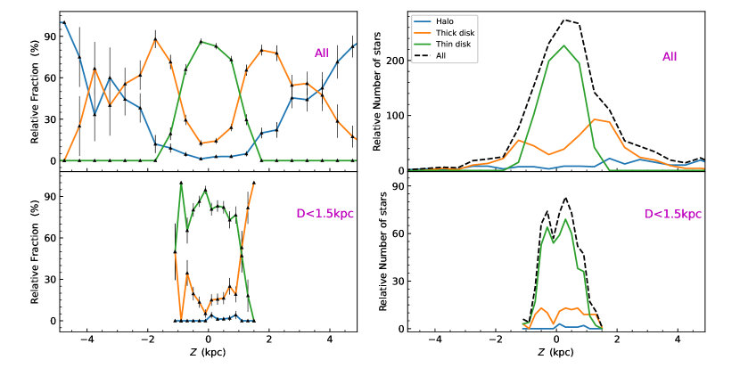
Figure 15 exhibits the relative fractional distributions of the 1587 Galactic halo, thick disk and thin disk population in Z distances for the four hot subdwarf helium abundance classes. The 1.5 kpc distance limit barely reaches the halo, therefore the relative errors for the halo population are large within the restricted volume-limited sample. The comparison of the 1587 star sample to the volume-limited sample in Figure 16 reveals the extent of the disk populations. The thin disk dominates the observed population over kpc and shows a nearly symmetric distribution to the mid-plane of the Galaxy. The contribution of the thick disk population is as low as 10% of all stars at the mid-plane, rises rapidly and over kpc it dominates over the thin disk. The thick disk reaches its peak at kpc, where the thin disk is negligible. The decline of the relative contribution of thick disk stars is much slower and their distribution resembles a Maxwell-Boltzmann distribution. The halo population is very low, below 2% in the mid-plane, and rises slowly. Due to the low number statistics, the halo contribution can be determined much less accurately, but it dominates over the thick disk population beyond kpc.
The bright stars in a magnitude limited sample allow one to explore the extent of the disk populations on larger scales. When the volume-limited sample is considered (bottom panels in Figure 16, these bright stars are neglected and the double peak of the thick disk distribution remains poorly and partially covered. The sample at kpc and within kpc is limited to a few stars at very high galactic latitudes. The halo contribution to the volume-limited sample is almost negligible (8 out of 590). However, the relative fractions found in the volume-limited sample confirm the observations made in the 1587 star sample, 85% of stars in the midplane belong to the thin disk and about 14% belong to the thick disk and about 1% belongs to the halo. The two disk populations have equal contributions at kpc, just like in the 1587 star sample. The volume-limited distribution looks boxier because the distance limit cuts off high objects. If we take the 467 thin disk stars and 115 thick disk stars in the volume-limited sample and observe in Figure 16 that the majority of these are within kpc, we find the hot subdwarf number density is kpc-3 in the thin disk and kpc-3 in the thick disk, respectively.
We did not find significant differences among the correlations of atmospheric parameters of thin and thick disk stars. This may be in part due to the atmospheric properties of hot subdwarfs being independent of their progenitor stars. However, we expect a different bulk metallicity of these stars and, therefore, a difference in the total and core mass may exist and will be the subject of future work.
7 Conclusions
We identified 1587 hot subdwarf stars with LAMOST DR7 observations from the Gaia DR2 hot subdwarf candidate catalog (Geier et al., 2019), among which 224 are confirmed as hot subdwarfs for the first time. We obtained atmospheric parameters for these stars by fitting their LAMOST spectra with Tlusty/Synspec non-LTE synthetic spectra. Making use of the LAMOST radial velocities and the Gaia EDR3 parallaxes and proper motions, we presented the Galactic space positions, velocity vectors and orbital parameters. By combining the Galactic velocity components with orbital parameters, we calculated the Galactic population memberships of the stars and made a comparison with the Galactic globular cluster Cen. Following our previous works (Luo et al., 2019, 2020), these stars were divided into four classes depending on their He abundances. We summarize our results in Fig 17 as follows:
-
1.
The atmospheric parameters of our sample reproduce and confirm the two known He sequences of sdB stars in the diagram. According to our He classification scheme, our sample is divided into four He hot subdwarf classes in the and diagrams. Two groups (He-1 and He-2) can be outlined for He-rich stars with and another two groups (He-1 and He-2) for He-rich stars with . Group He-2 is a newly discovered group. Our comparisons with theoretical hot subdwarf formation models illustrate that the hot-flasher evolutionary tracks (Miller Bertolami et al., 2008) can match Groups He-2, He-1 and He-2, and the double WD merger model (Zhang & Jeffery, 2012) can explain the properties of Group He-1 and He-2. We associate Group He-1 with the fast merger channel and Group He-2 with the slow merger channel.
-
2.
The four He classes exhibit some noticeable differences in their space distributions, the Galactic velocity distributions and the Galactic orbital parameter distributions, which are clearly reflected in their Galactic population classifications. The two He-deficient classes show very similar contributions to the halo populations, while the two He-rich classes show no differences in their relative fractions in the thick disk and the halo. The halo population fractions of both He-rich classes are higher by than those of the He-deficient classes. The situation is the opposite for the thin disk population fractions, which suggests that He-rich and He-deficient stars have different formation channels. The two groups (He-1 and He-2) of He-rich stars with show significant differences in all three population fractions. Group He-1 constitutes of thin disk stars, thick disk stars and halo stars, while the corresponding fractions in Group He-2 are in the thin disk, in the thick disk and in the halo. These suggest that over half of the stars in Group He-1 are halo stars, but over half of stars in Group He-2 are thin disk stars. It is possible that these two groups are from different formation channels. The values of the thin and thick disk population fractions of Group He-1 are between those of Group He-1 and He-2. The halo population of Group He-1 is significantly higher than that of He-2 but it has no significant difference between Groups He-1 and He-2. Group He-1 is completely different from Group He-2 in the Galactic population fractions. The latter has no halo stars and shows thin disk population fraction and thick disk population fraction, which implies that Groups He-1 and He-2 have different formation channels.
-
3.
The relative fractions of the four hot subdwarf helium classes in the halo, thin disk and thick disk can be largely matched with our previous results (Luo et al., 2019, 2020), which appears to support the predictions of binary population synthesis (Han et al., 2003; Han, 2008). He-weak stars with are likely originate from the stable RLOF channel, He-poor stars with are from the CE ejection channel and He-rich stars with are from the merger channel of double HeWDs. The comparisons between hot subdwarf stars in the halo and the globular cluster Cen show that of the four He classes, except for the He-weak class with , have a significant difference in their relative population fractions. Both the He-rich class with and the He-poor class with are two times smaller in the halo field than in Cen. The relative fraction of He-rich stars with in Cen is four times of that in the halo field. These results suggest that the particular cluster environment has little effect on the formation of He-deficient stars formed by the RLOF channel, but it does significantly cut the formation of hot subdwarf stars through the double WD merger and CE ejection channels and significantly contribute to the formation of He-rich stars with in spite of their puzzling origin. We find that He-rich stars with discovered in Cen are missing in the thick disk and halo, but they appear in the thin disk, which indicates that these stars may have a similar formation channel in the thin disk and Cen.
-
4.
We have found substantial differences among hot subdwarf He abundance classes and groups. By combining these differences with kinematic properties, we see a fragmentation of the galactic hot subdwarf population. There are different dichotomies between the thick and thin disk populations, and the halo and Cen populations of stars. It is the scope of future research to find if the observed dichotomies are present due to differences in stellar and binary evolution in different galactic environments, or due to a dilution of disk stars by a past major merger of the Milky Way with a satellite galaxy. By simple population membership considerations, we found a hot subdwarf number density of kpc-3 in the thin disk and kpc-3 in the thick disk for the solar neighborhood, respectively. We did not find significant differences among the correlations of atmospheric parameters of thin and thick disk stars. However, we expect a different bulk metallicity of these stars and a difference in the total and core mass may exist.
References
- Astropy Collaboration et al. (2013) Astropy Collaboration, Robitaille, T. P., Tollerud, E. J., et al. 2013, A&A, 558, A33. doi:10.1051/0004-6361/201322068
- Astropy Collaboration et al. (2018) Astropy Collaboration, Price-Whelan, A. M., Sipőcz, B. M., et al. 2018, AJ, 156, 123. doi:10.3847/1538-3881/aabc4f
- Bailer-Jones et al. (2018) Bailer-Jones, C. A. L., Rybizki, J., Fouesneau, M., et al. 2018, AJ, 156, 58. doi:10.3847/1538-3881/aacb21
- Bailer-Jones et al. (2021) Bailer-Jones, C. A. L., Rybizki, J., Fouesneau, M., et al. 2021, AJ, 161, 147. doi:10.3847/1538-3881/abd806
- Bovy (2015) Bovy, J. 2015, ApJS, 216, 29. doi:10.1088/0067-0049/216/2/29
- Byrne et al. (2018) Byrne, C. M., Jeffery, C. S., Tout, C. A., et al. 2018, MNRAS, 475, 4728. doi:10.1093/mnras/sty158
- Charpinet et al. (2010) Charpinet, S., Green, E. M., Baglin, A., et al. 2010, A&A, 516, L6. doi:10.1051/0004-6361/201014789
- Cui et al. (2012) Cui, X.-Q., Zhao, Y.-H., Chu, Y.-Q., et al. 2012, Research in Astronomy and Astrophysics, 12, 1197. doi:10.1088/1674-4527/12/9/003
- D’Cruz et al. (1996) D’Cruz, N. L., Dorman, B., Rood, R. T., et al. 1996, ApJ, 466, 359. doi:10.1086/177515
- Drilling et al. (2013) Drilling, J. S., Jeffery, C. S., Heber, U., et al. 2013, A&A, 551, A31. doi:10.1051/0004-6361/201219433
- Dorman et al. (1993) Dorman, B., Rood, R. T., & O’Connell, R. W. 1993, ApJ, 419, 596. doi:10.1086/173511
- Dorsch et al. (2019) Dorsch, M., Latour, M., & Heber, U. 2019, A&A, 630, A130. doi:10.1051/0004-6361/201935724
- Dorsch et al. (2020) Dorsch, M., Latour, M., Heber, U., et al. 2020, A&A, 643, A22. doi:10.1051/0004-6361/202038859
- Edelmann et al. (2003) Edelmann, H., Heber, U., Hagen, H.-J., et al. 2003, A&A, 400, 939. doi:10.1051/0004-6361:20030135
- Fernández-Menchero et al. (2020) Fernández-Menchero, L., Jeffery, C. S., Ramsbottom, C. A., et al. 2020, MNRAS, 496, 2558. doi:10.1093/mnras/staa1710
- Gaia Collaboration et al. (2016) Gaia Collaboration, Prusti, T., de Bruijne, J. H. J., et al. 2016, A&A, 595, A1. doi:10.1051/0004-6361/201629272
- Gaia Collaboration et al. (2018) Gaia Collaboration, Brown, A. G. A., Vallenari, A., et al. 2018, A&A, 616, A1. doi:10.1051/0004-6361/201833051
- Gaia Collaboration et al. (2020) Gaia Collaboration, Brown, A. G. A., Vallenari, A., et al. 2020, arXiv:2012.01533
- Geier et al. (2013) Geier, S., Marsh, T. R., Wang, B., et al. 2013, A&A, 554, A54. doi:10.1051/0004-6361/201321395
- Geier et al. (2015) Geier, S., Fürst, F., Ziegerer, E., et al. 2015, Science, 347, 1126. doi:10.1126/science.1259063
- Geier et al. (2015) Geier, S., Kupfer, T., Heber, U., et al. 2015, A&A, 577, A26. doi:10.1051/0004-6361/201525666
- Geier et al. (2019) Geier, S., Raddi, R., Gentile Fusillo, N. P., et al. 2019, A&A, 621, A38. doi:10.1051/0004-6361/201834236
- Geier (2020) Geier, S. 2020, A&A, 635, A193. doi:10.1051/0004-6361/202037526
- Han et al. (2002) Han, Z., Podsiadlowski, P., Maxted, P. F. L., et al. 2002, MNRAS, 336, 449. doi:10.1046/j.1365-8711.2002.05752.x
- Han et al. (2003) Han, Z., Podsiadlowski, P., Maxted, P. F. L., et al. 2003, MNRAS, 341, 669. doi:10.1046/j.1365-8711.2003.06451.x
- Han et al. (2007) Han, Z., Podsiadlowski, P., & Lynas-Gray, A. E. 2007, MNRAS, 380, 1098. doi:10.1111/j.1365-2966.2007.12151.x
- Han (2008) Han, Z. 2008, A&A, 484, L31. doi:10.1051/0004-6361:200809614
- Han et al. (2020) Han, Z.-W., Ge, H.-W., Chen, X.-F., et al. 2020, Research in Astronomy and Astrophysics, 20, 161. doi:10.1088/1674-4527/20/10/161
- Heber (2009) Heber, U. 2009, ARA&A, 47, 211. doi:10.1146/annurev-astro-082708-101836
- Heber (2016) Heber, U. 2016, PASP, 128, 082001. doi:10.1088/1538-3873/128/966/082001
- Hirsch (2009) Hirsch, H. A. 2009, Ph.D. Thesis,Friedrich-Alexander University Erlangen-Nürnberg
- Hubeny & Lanz (1995) Hubeny, I. & Lanz, T. 1995, ApJ, 439, 875. doi:10.1086/175226
- Hubeny & Lanz (2011) Hubeny, I. & Lanz, T. 2011, Astrophysics Source Code Library. ascl:1109.022
- Hubeny & Lanz (2017a) Hubeny, I. & Lanz, T. 2017, arXiv:1706.01859
- Hubeny & Lanz (2017b) Hubeny, I. & Lanz, T. 2017, arXiv:1706.01935
- Hubeny & Lanz (2017c) Hubeny, I. & Lanz, T. 2017, arXiv:1706.01937
- Irrgang et al. (2013) Irrgang, A., Wilcox, B., Tucker, E., et al. 2013, A&A, 549, A137. doi:10.1051/0004-6361/201220540
- Ivanova et al. (2013) Ivanova, N., Justham, S., Chen, X., et al. 2013, A&A Rev., 21, 59. doi:10.1007/s00159-013-0059-2
- Jeffery et al. (2017) Jeffery, C. S., Baran, A. S., Behara, N. T., et al. 2017, MNRAS, 465, 3101. doi:10.1093/mnras/stw2852
- Jeffery & Miszalski (2019) Jeffery, C. S. & Miszalski, B. 2019, MNRAS, 489, 1481. doi:10.1093/mnras/stz2231
- Jeffery (2020) Jeffery, C. S. 2020, MNRAS, 496, 718. doi:10.1093/mnras/staa1555
- Jeffery et al. (2021) Jeffery, C. S., Miszalski, B., & Snowdon, E. 2021, MNRAS, 501, 623. doi:10.1093/mnras/staa3648
- Justham et al. (2009) Justham, S., Wolf, C., Podsiadlowski, P., et al. 2009, A&A, 493, 1081. doi:10.1051/0004-6361:200810106
- Kawka et al. (2015) Kawka, A., Vennes, S., O’Toole, S., et al. 2015, MNRAS, 450, 3514. doi:10.1093/mnras/stv821
- Kupfer et al. (2015) Kupfer, T., Geier, S., Heber, U., et al. 2015, A&A, 576, A44. doi:10.1051/0004-6361/201425213
- Kupfer et al. (2019) Kupfer, T., Bauer, E. B., Burdge, K. B., et al. 2019, ApJ, 878, L35. doi:10.3847/2041-8213/ab263c
- Kepler et al. (2019) Kepler, S. O., Pelisoli, I., Koester, D., et al. 2019, MNRAS, 486, 2169. doi:10.1093/mnras/stz960
- Latour et al. (2018) Latour, M., Chayer, P., Green, E. M., et al. 2018, A&A, 609, A89. doi:10.1051/0004-6361/201731496
- Latour et al. (2018) Latour, M., Randall, S. K., Calamida, A., et al. 2018, A&A, 618, A15. doi:10.1051/0004-6361/201833129
- Lei et al. (2013) Lei, Z.-X., Chen, X.-F., Zhang, F.-H., et al. 2013, A&A, 549, A145. doi:10.1051/0004-6361/201220238
- Lei et al. (2015) Lei, Z., Chen, X., Zhang, F., et al. 2015, MNRAS, 449, 2741. doi:10.1093/mnras/stv544
- Lei et al. (2018) Lei, Z., Zhao, J., Németh, P., et al. 2018, ApJ, 868, 70. doi:10.3847/1538-4357/aae82b
- Lei et al. (2019) Lei, Z., Zhao, J., Németh, P., et al. 2019, ApJ, 881, 135. doi:10.3847/1538-4357/ab2edc
- Lei et al. (2020) Lei, Z., Zhao, J., Németh, P., et al. 2020, ApJ, 889, 117. doi:10.3847/1538-4357/ab660a
- Lisker et al. (2005) Lisker, T., Heber, U., Napiwotzki, R., et al. 2005, A&A, 430, 223. doi:10.1051/0004-6361:20040232
- Luo et al. (2012) Luo, A.-L., Zhang, H.-T., Zhao, Y.-H., et al. 2012, Research in Astronomy and Astrophysics, 12, 1243. doi:10.1088/1674-4527/12/9/004
- Luo et al. (2014) Luo, A., Zhang, J., Chen, J., et al. 2014, Setting the scene for Gaia and LAMOST, 298, 428. doi:10.1017/S1743921313006947
- Luo et al. (2016) Luo, Y.-P., Németh, P., Liu, C., et al. 2016, ApJ, 818, 202. doi:10.3847/0004-637X/818/2/202
- Luo et al. (2019) Luo, Y., Németh, P., Deng, L., et al. 2019, ApJ, 881, 7. doi:10.3847/1538-4357/ab298d
- Luo et al. (2020) Luo, Y., Németh, P., & Li, Q. 2020, ApJ, 898, 64. doi:10.3847/1538-4357/ab98f3
- Ma et al. (2017) Ma, X., Hopkins, P. F., Wetzel, A. R., et al. 2017, MNRAS, 467, 2430. doi:10.1093/mnras/stx273
- Martin et al. (2017) Martin, P., Jeffery, C. S., Naslim, N., et al. 2017, MNRAS, 467, 68. doi:10.1093/mnras/stw3305
- Mihalas et al. (1974) Mihalas, D., Barnard, A. J., Cooper, J., et al. 1974, ApJ, 190, 315. doi:10.1086/152878
- Miller Bertolami et al. (2008) Miller Bertolami, M. M., Althaus, L. G., Unglaub, K., et al. 2008, A&A, 491, 253. doi:10.1051/0004-6361:200810373
- Moehler et al. (2004) Moehler, S., Sweigart, A. V., Landsman, W. B., et al. 2004, A&A, 415, 313. doi:10.1051/0004-6361:20034505
- Naslim et al. (2011) Naslim, N., Jeffery, C. S., Behara, N. T., et al. 2011, MNRAS, 412, 363. doi:10.1111/j.1365-2966.2010.17909.x
- Naslim et al. (2013) Naslim, N., Jeffery, C. S., Hibbert, A., et al. 2013, MNRAS, 434, 1920. doi:10.1093/mnras/stt1091
- Naslim et al. (2020) Naslim, N., Jeffery, C. S., & Woolf, V. M. 2020, MNRAS, 491, 874. doi:10.1093/mnras/stz3055
- Németh et al. (2012) Németh, P., Kawka, A., & Vennes, S. 2012, MNRAS, 427, 2180. doi:10.1111/j.1365-2966.2012.22009.x
- Németh et al. (2016) Németh, P., Ziegerer, E., Irrgang, A., et al. 2016, ApJ, 821, L13. doi:10.3847/2041-8205/821/1/L13
- Østensen et al. (2014) Østensen, R. H., Telting, J. H., Reed, M. D., et al. 2014, A&A, 569, A15. doi:10.1051/0004-6361/201423611
- Østensen et al. (2020) Østensen, R. H., Jeffery, C. S., Saio, H., et al. 2020, MNRAS, 499, 3738. doi:10.1093/mnras/staa3123
- Paczyński (1971) Paczyński, B. 1971, Acta Astron., 21, 1
- Pauli et al. (2003) Pauli, E.-M., Napiwotzki, R., Altmann, M., et al. 2003, A&A, 400, 877. doi:10.1051/0004-6361:20030012
- Pauli et al. (2006) Pauli, E.-M., Napiwotzki, R., Heber, U., et al. 2006, A&A, 447, 173. doi:10.1051/0004-6361:20052730
- Pelisoli et al. (2020) Pelisoli, I., Vos, J., Geier, S., et al. 2020, A&A, 642, A180. doi:10.1051/0004-6361/202038473
- Ratzloff et al. (2020) Ratzloff, J. K., Kupfer, T., Barlow, B. N., et al. 2020, ApJ, 902, 92. doi:10.3847/1538-4357/abb5b2
- Sahoo et al. (2020) Sahoo, S. K., Baran, A. S., Heber, U., et al. 2020, MNRAS, 495, 2844. doi:10.1093/mnras/staa1337
- Saio & Jeffery (2019) Saio, H. & Jeffery, C. S. 2019, MNRAS, 482, 758. doi:10.1093/mnras/sty2763
- Schoening & Butler (1989) Schoening, T. & Butler, K. 1989, A&AS, 78, 51
- Schönrich et al. (2010) Schönrich, R., Binney, J., & Dehnen, W. 2010, MNRAS, 403, 1829. doi:10.1111/j.1365-2966.2010.16253.x
- Stroeer et al. (2007) Stroeer, A., Heber, U., Lisker, T., et al. 2007, A&A, 462, 269. doi:10.1051/0004-6361:20065564
- Taylor (2005) Taylor, M. B. 2005, Astronomical Data Analysis Software and Systems XIV, 347, 29
- Taylor (2019) Taylor, M. B. 2019, Astronomical Data Analysis Software and Systems XXVII, 523, 43
- Tremblay & Bergeron (2009) Tremblay, P.-E. & Bergeron, P. 2009, ApJ, 696, 1755. doi:10.1088/0004-637X/696/2/1755
- Xiang et al. (2017) Xiang, M., Liu, X., Shi, J., et al. 2017, ApJS, 232, 2. doi:10.3847/1538-4365/aa80e4
- Vos et al. (2020) Vos, J., Bobrick, A., & Vučković, M. 2020, A&A, 641, A163. doi:10.1051/0004-6361/201937195
- Wang et al. (2009) Wang, B., Meng, X., Chen, X., et al. 2009, MNRAS, 395, 847. doi:10.1111/j.1365-2966.2009.14545.x
- Wang & Han (2010) Wang, B. & Han, Z. 2010, A&A, 515, A88. doi:10.1051/0004-6361/200913976
- Webbink (1984) Webbink, R. F. 1984, ApJ, 277, 355. doi:10.1086/161701
- Wu et al. (2018) Wu, Y., Chen, X., Li, Z., et al. 2018, A&A, 618, A14. doi:10.1051/0004-6361/201832686
- Wu et al. (2020) Wu, Y., Chen, X., Chen, H., et al. 2020, A&A, 634, A126. doi:10.1051/0004-6361/201935792
- Zhang & Jeffery (2012) Zhang, X. & Jeffery, C. S. 2012, MNRAS, 419, 452. doi:10.1111/j.1365-2966.2011.19711.x
- Zhang et al. (2017) Zhang, X., Hall, P. D., Jeffery, C. S., et al. 2017, ApJ, 835, 242. doi:10.3847/1538-4357/835/2/242
- Zong et al. (2018) Zong, W., Charpinet, S., Fu, J.-N., et al. 2018, ApJ, 853, 98. doi:10.3847/1538-4357/aaa548


| Num | Label | Explanations |
|---|---|---|
| 1 | LAMOST | LAMOST target |
| 2 | Barycentric Right Ascension (J2000) (1)(1)At Epoch 2000.0 (ICRS). | |
| 3 | Barycentric Declination (J2000) (1)(1)At Epoch 2000.0 (ICRS). | |
| 4 | Stellar effective temperature | |
| 5 | Standard error in | |
| 6 | Stellar surface gravity | |
| 7 | Standard error of Stellar surface gravity | |
| 8 | Stellar surface He abundance | |
| 9 | Standard error in | |
| 10 | Gaia EDR3 proper motion in RA | |
| 11 | Standard error | |
| 12 | Gaia EDR3 proper motion in DE | |
| 13 | Standard error in | |
| 14 | Gaia EDR3 stellar distance | |
| 15 | Standard error in stellar distance | |
| 16 | Radial velocity from LAMOST spectra | |
| 17 | Standard error in radial velocity | |
| 18 | Galactic position towards Galactic center | |
| 19 | Standard error in | |
| 20 | Galactic position along Galactic rotation | |
| 21 | Standard error of | |
| 22 | Galactic position towards north Galactic pole | |
| 23 | Standard error of | |
| 24 | Galactic radial velocity positive towards Galactic center | |
| 25 | Standard error in | |
| 26 | Galactic rotational velocity along Galactic rotation | |
| 27 | Standard error in | |
| 28 | Galactic velocity towards north Galactic pole | |
| 29 | Standard error in | |
| 30 | Apocenter radius (2)(2)Form the numerical orbit integration. | |
| 31 | Standard error in | |
| 32 | Pericenter radius (2)(2)Form the numerical orbit integration. | |
| 33 | Standard error in | |
| 34 | Maximum vertical height (2)(2)Form the numerical orbit integration. | |
| 35 | Standard error in | |
| 36 | Eccentricity (2)(2)Form the numerical orbit integration. | |
| 37 | Standard error in | |
| 38 | Zcomponent of angular momentum (2)(2)Form the numerical orbit integration. | |
| 39 | Standard error in | |
| 40 | Normalised z-extent of the orbit (2)(2)Form the numerical orbit integration. | |
| 41 | Standard error in | |
| 42 | Groupid | Group name for He-rich stars (3)(3)1He-1; 1He-2; 3He-1; 4He-2. |
| 43 | Pops | Population classification (4)(4)HHalo; TKthick disk; THthin disk. |
| 44 | probability in thin disk | |
| 45 | probability in thick disk | |
| 46 | probability in halo | |
| 47 | Newsample | New hot subdwarf star identified in LAMOST DR7 (5)(5)YYes; NNo. |
Note. — The full table can be found in the online version of the paper.
| Num | Label | Explanations |
|---|---|---|
| 1 | LAMOST | LAMOST target |
| 2 | GaiaEDR3 | Unique Gaia EDR3 source identifier |
| 3 | Barycentric Right Ascension (J2000) (1)(1)At Epoch 2000.0 (ICRS). | |
| 4 | Barycentric Declination (J2000) (1)(1)At Epoch 2000.0 (ICRS). | |
| 5 | Gaia EDR3 stellar parallax | |
| 6 | Standard error in | |
| 7 | Gaia EDR3 proper motion in RA | |
| 8 | Standard error | |
| 9 | Gaia EDR3 proper motion in DE | |
| 10 | Standard error in | |
| 11 | Gaia EDR3 Gband magnitude | |
| 12 | Gaia EDR3 colour | |
| 13 | SpClass | Spectra classification (photBpMeanMagphotRpMeanMag) (2)(2)spectral classes are as follows: BHB Blue Horizontal Branch star; CV Cataclysmic Variable star; DA white dwarfs with H lines only; DB white dwarfs with neutral He lines only; MSB B type main sequence star; MSA A type main sequence star; sdA A type subdwarf star; sdMS hot subdwarfMain Sequence binary candidates; UNK Bad spectra which we were unable to classify; Unreliable Spectra with low signal. |
Note. — The full table can be found in the online version of the paper.
| Subsample | N | ||||||||||||||||||||
|---|---|---|---|---|---|---|---|---|---|---|---|---|---|---|---|---|---|---|---|---|---|
| All stars | 1587 | 14 | 62 | 198 | 47 | -1 | 38 | 214 | 42 | 0.24 | 0.16 | 1763.74 | 598.04 | 0.13 | 0.10 | 1.30 | 0.94 | 10.21 | 1.91 | 6.12 | 2.61 |
| He | 803 | 15 | 61 | 203 | 44 | -1 | 35 | 216 | 40 | 0.23 | 0.14 | 1824.73 | 525.26 | 0.12 | 0.09 | 1.21 | 0.84 | 10.18 | 1.90 | 6.25 | 2.47 |
| He | 472 | 12 | 58 | 198 | 47 | -1 | 38 | 212 | 41 | 0.24 | 0.15 | 1783.13 | 589.84 | 0.13 | 0.10 | 1.33 | 0.97 | 10.13 | 1.74 | 6.23 | 2.58 |
| He | 90 | 8 | 82 | 173 | 72 | -10 | 48 | 206 | 52 | 0.36 | 0.26 | 1456.57 | 826.99 | 0.16 | 0.14 | 2.20 | 2.09 | 10.02 | 1.92 | 5.35 | 2.88 |
| He | 222 | 15 | 87 | 181 | 58 | -2 | 40 | 209 | 45 | 0.34 | 0.26 | 1550.70 | 866.36 | 0.18 | 0.14 | 1.72 | 1.32 | 10.45 | 2.11 | 5.74 | 3.01 |
| He-1 | 69 | -8 | 90 | 166 | 70 | -15 | 49 | 204 | 51 | 0.37 | 0.28 | 1429.64 | 938.69 | 0.23 | 0.16 | 2.34 | 1.56 | 10.58 | 2.36 | 5.36 | 3.15 |
| He-2 | 71 | 13 | 76 | 196 | 42 | -1 | 27 | 214 | 35 | 0.25 | 0.18 | 1769.81 | 494.10 | 0.11 | 0.08 | 1.11 | 0.73 | 10.03 | 1.72 | 6.05 | 2.51 |
| He-1 | 65 | 7 | 82 | 167 | 70 | -9 | 55 | 203 | 50 | 0.38 | 0.28 | 1358.52 | 816.37 | 0.19 | 0.17 | 2.40 | 2.17 | 9.64 | 1.47 | 5.07 | 2.84 |
| He-2 | 17 | 12 | 50 | 238 | 27 | -3 | 17 | 244 | 24 | 0.14 | 0.06 | 2244.47 | 350.01 | 0.06 | 0.03 | 0.68 | 0.43 | 11.09 | 1.96 | 8.32 | 1.57 |
| Subsample | N | Thin Disk | Thick Disk | Halo |
|---|---|---|---|---|
| All stars | 1587 | 779 | 568 | 240 |
| He | 803 | 426 | 269 | 108 |
| He | 472 | 233 | 183 | 56 |
| He | 90 | 34 | 31 | 25 |
| He | 222 | 86 | 85 | 51 |
| He-1 | 69 | 15 | 38 | 16 |
| He-2 | 71 | 36 | 24 | 11 |
| He-1 | 65 | 25 | 22 | 18 |
| He-2 | 17 | 15 | 2 | 0 |